A model for pricing real estate derivatives with stochastic interest rates

Munich Personal RePEc Archive

A model for pricing real estate

derivatives with stochastic interest rates

Ciurlia, Pierangelo and Gheno, Andrea

Department of Economics, University of Rome III, Rome, Italy

8 August 2008

Online at

https://mpra.ub.uni-muenchen.de/9924/

A model for pricing real estate derivatives

with stochastic interest rates

P. Ciurlia

, A. Gheno

∗

a_{Department of Economics, University of Rome III, Rome, Italy}

Abstract

The real estate derivatives market allows participants to manage risk and return from exposure to property, without buying or selling directly the underlying asset. Such market is growing very fast hence the need to rely on simple yet effective pricing models is very great. In order to take into account the real estate market sensitivity to the interest rate term structure in this paper is presented a two-factor model where the real estate asset value and the spot rate dynamics are jointly modeled. The pricing problem for both European and American options is then analyzed and since no closed-form solution can be found a bidimensional binomial lattice framework is adopted. The model proposed allows calibration to the interest rate and volatility term structures.

Key words: Real estate; derivatives pricing; stochastic interest rate; bidimensional binomial lattice.

1 Introduction

The derivatives pricing problem roots lie in the seminal papers by Black and Scholes [1] and Merton [2] (hereafter BSM). They were the first to analytically solve the option pricing problem and for this achievement in 1997 were awarded the Nobel prize. This paper relies on the BSM risk-neutral valuation framework adapting it to the peculiarity of the real estate derivatives. In fact this class of contracts is characterized by a payoff dependent on an underlying real estate asset whose value depends on the interest rate dynamics. In particular in this paper the real estate asset value is represented by a geometric Brownian

∗ _{Corresponding author.}

motion whereas the spot interest rate, which in the standard BSM framework is considered as a constant parameter, is properly modeled as a stochastic variable.

The layout of the remainder of the paper is as follows. In section 2 we present the two-factor pricing model in continuous time and derive the general valuation equation for any real estate derivative depending on the real estate asset value and the spot interest rate. Since the level of analytical tractability of the continuous-time model is quite limited, a discrete-time version within a bidimensional binomial lattice framework is introduced. In section 3 we show how the bidimensional binomial lattice can be implemented by using state-contingent Arrow-Debreu prices and then calibrated to the current market term structure of interest rates and the current term structure of volatilities. In section 4 an application to European and American option pricing problems is given. Finally conclusions are drawn in section 5.

2 Model formulation

Let us consider an economy with two correlated state variables, the real

estate asset value X = _{X(t), t _≥ 0_} and the risk-free spot interest rate

r =_{r(t), t_≥ 0_}, whose evolutions as function of the time variable t are

de-scribed respectively by the following stochastic differential equations (SDEs)

dX(t) = µX(Xt, t)dt+σX(Xt, t)dW1(t),

dr(t) =µr(rt, t)dt+σr(r_t, t)dW₂(t),

where _{Wi(t), t _≥0_}, for i= 1,2, are two standard Wiener processes defined

under the same natural probability measureP and correlated through a

time-dependent correlation coefficientρ(t)_∈[₋1,1],_∀t _≥0.

In particular, for the real estate asset value X we specify a geometric

Brownian motion

dX(t) = (µ₋δ)X(t)dt + σXX(t)dW1(t), (2.1)

whereδ _≥0 is the cash-flow continuously paid by the real estate asset andµis

its total expected rate of return, so that the difference µ₋δ is the real estate

asset rate of appreciation per unit time. The coefficient σX > 0 indicates the

instantaneous volatility of the real estate asset value.

The term structure is generated by a stochastic process modeling the

dlnr(t) = (

∂lnu(t)

∂t −

∂lnσr(t)

∂t

·

lnu(t)₋lnr(t)

¸)

dt

+σr(t)dW₂(t), (2.2)

where u(t) is the median of the spot rate distribution at time t and σr(t) the

spot rate volatility at time t. The spot rate process (2.2) is the

continuous-time equivalent of the interest rate model developed by Black, Derman and Toy [3] (hereafter called BDT model).

Although the BDT model was originally presented in a discrete-time bino-mial lattice framework, equation (2.2) better clarifies the distinctive features of this arbitrage-free and yield-based model. In fact the two unknown

time-dependent functions, u(t) and σr(t), are chosen to make the model consistent

with, respectively, the current market term structure of interest rates (also known as the yield curve) and the current term structure of volatilities (also known as the volatility curve). A further advantage with respect to other term structure models is that interest rates cannot become negative, since changes in spot rates are lognormally distributed. Unfortunately, due to its lognormality, no analytic solution can be found and thus numerical techniques are required to derive an interest rate tree that correctly matches the market term structures. An uncomfortable consequence of the model is that for

cer-tain specification of the volatility function σr(t) the spot interest rate can be

mean-fleeing rather than mean-reverting. For this reason, many practitioners find it better to fit the model only to the interest rate term structure, holding

the volatility term structure to a constant levelσr. In this case the stochastic

process (2.2) reduces to the following

dlnr(t) = ∂lnu(t)

∂t dt + σrdW2(t). (2.3)

Applying Itˆo’s lemma to (2.2) and assuming a risk-neutral valuation

set-ting1 _{the two-factor model can be written in matrix form as follows}



  

dX(t)

dr(t)    =     ³

r(t)₋δ´X(t) µ

ψ(t) + 1 2σr(t)2

¶

r(t) 

 

dt +



  

σXX(t) 0

0 σr(t)2r(t)

       

dW˜1(t)

dW˜2(t) 

 

,

with

1 _{For more details on risk-neutral valuation and real estate derivatives see [4] where}

ψ(t) =∂lnu(t)

∂t −

∂lnσr(t)

∂t

·

lnu(t)₋lnr(t) ¸

,

and where the terms dW˜1(t) anddW˜2(t) are increments of the two correlated

standard Wiener processes defined now under the risk-neutral probability

mea-sure Q.

Let Π(t) = Π(Xt, rt, t) be a continuous, twice-differentiable function of the

state variables X and r at timet, and differentiable with respect to the time

variable t. Applying the multivariate version of Itˆo’s Lemma, we have

dΠ(t) = "

∂Π(t)

∂t + ∂Π(t)

∂X

³

r(t)₋δ´X(t) + ∂Π(t)

∂r

µ

ψ(t) + 1

2σ

2

r(t)

¶

r(t)

+ 1

2

∂2_Π(t)

∂X2 σ 2

XX(t)

2₊1 2

∂2_Π(t)

∂r2 σr(t)

2_r(t)2

+ ∂

2_Π(t)

∂X∂r ρ(t)σXσr(t)X(t)r(t)

#

dt

+∂Π(t)

∂X σXX(t)dW˜1(t) +

∂Π(t)

∂r σr(t)r(t)dW˜2(t).

Using the hedging argument yields the following second-order partial differ-ential equation

∂Π(t)

∂t + ∂Π(t)

∂X

³

r(t)₋δ´X(t) + ∂Π(t)

∂r

" µ

ψ(t) + 1 2σr(t)

2¶

+q(t)σr(t)

#

r(t) + 1 2

∂2_Π(t)

∂X2 σ 2

XX(t)

2₊ 1 2

∂2_Π(t)

∂r2 σr(t)2r(t)2

+∂

2_Π(t)

∂X∂r ρ(t)σXσr(t)X(t)r(t)−r(t)Π(t) = 0, (2.4)

where q(t) is the market price of the interest-rate risk. In order to determine

the value Π of any contingent claim dependent upon X and r, we must solve

numerically equation (2.4), subject to the appropriate terminal and boundary conditions.

For computational purposes it is convenient to approximate the joint

evo-lution of the two continuous-time stochastic processes X and r with a

bidi-mensional binomial (BB) lattice. In order to specify the jump sizes and prob-abilities we equate means, variances and correlations for the bidimensional

binomial process with those of the stochastic processes X and r. Given that

dy(t) =ν(t)dt + σXdW˜1(t), (2.5)

where y(t) := lnX(t) and with the drift term ν(t) which is defined as

ν(t) = µ

r(t)₋δ₋ 1

2σ

2

X

¶

.

Let us assume that during the time period [t, t+∆t] the natural logarithms

ofX andrcan either go up to levels respectively of y(t) + ∆yu(t) and lnr(t) + ∆ lnru(t) or down to levels respectively ofy(t)+∆yd(t) and lnr(t)+∆ lnrd(t). Letpuu(t),pud(t),pdu(t) andpdd(t) denote the joint probabilities of the additive up and down jumps for the BB process, with the two subscripts representing

the jump type, upwarduor downwardd, ofyand lnr, respectively. The

time-dependent sets of additive jump sizes _{∆yu(t), ∆yd(t), ∆ lnru(t), ∆ lnrd(t)_} and joint probabilities _{puu(t), pud(t), pdu(t), pdd(t)} are chosen to match the first and the second moments of the risk-neutral processes, i.e.,

E³∆y(t)´:=³puu(t) +pud(t)´∆yu(t) +³pdu(t) +pdd(t)´∆yd(t)

=ν(t)∆t, (2.6)

E³∆y(t)2´:=³puu(t) +pud(t)´∆yu(t)2 +³pdu(t) +pdd(t)´∆yd(t)2

=σ2X∆t+ν(t)

2_∆t2_{, (2.7)}

E³∆ lnr(t)´:=³puu(t) +pdu(t) ´

∆ lnru(t) + ³

pud(t) +pdd(t) ´

∆ lnrd(t)

=ψ(t)∆t, (2.8)

E³∆ lnr(t)2´:=³puu(t) +pdu(t)´∆ lnr_u2+³pud(t) +pdd(t)´∆ lnr2_d

=σr(t)2∆t+ψ(t)2∆t2, (2.9)

E³∆y(t)∆ lnr(t)´:=³puu(t)₋pdu(t)´∆y(t)∆ lnru(t) +³pud(t)₋pdd(t)´∆y(t)∆ lnrd(t)

=ρ(t)σXσr(t)∆t+ν(t)ψ(t)∆t2, (2.10)

where the joint probabilities must satisfy the following constraint

puu(t) +pud(t) +pdu(t) +pdd(t) = 1. (2.11)

Note that the system of equations listed above cannot be solved analyti-cally since there are more unknowns than constraints. In order to ensure the analytical tractability of the model we set the upward and downward jump

∆yu(t) = ₋∆yd(t) with ∆yu(t)_≡∆y(t). (2.12)

The above condition is similar to that originally proposed by [5] and on aver-age has slightly better accuracy than the standard univariate binomial model with equal probabilities of one-half developed by [6]. Finally, we impose that the unconditional probabilities of upward and downward jumps for the short-rate dynamics are both equal to one-half. This choice in conjunction with equation (2.11) leads to the following constraints

puu(t) +pdu(t) := pr =

1

2, (2.13)

pud(t) +pdd(t) = 1₋pr :=qr =

1

2. (2.14)

Since the system consisting of equations (2.6)-(2.10) and (2.12)-(2.14) can

now be solved analytically, we obtain for the additive jump sizes, ∆y(t),

∆ lnru(t) and ∆ lnrd(t), and the joint probabilities, puu(t), pud(t), pdu(t), and

pdd(t), the following expressions in terms of model parameters

∆y(t) =qσ2

X∆t+ν(t)2∆t2, (2.15)

∆ lnru(t) = ψ(t)∆t+σr(t)

√

∆t, (2.16)

∆ lnrd(t) =ψ(t)∆t₋σr(t)

√

∆t, (2.17)

and

puu(t) = 1 4



1 +

ν(t)√∆t

q

σ2

X +ν(t)2∆t

+ ρ(t)σX

q

σ2

X +ν(t)2∆t



, (2.18)

pud(t) = 1 4



1 +

ν(t)√∆t

q

σ2

X +ν(t)2∆t

− ρ(t)σX

q

σ2

X +ν(t)2∆t



, (2.19)

pdu(t) = 1 4



1−

ν(t)√∆t

q

σ2

X +ν(t)2∆t

− ρ(t)σX

q

σ2

X +ν(t)2∆t



, (2.20)

pdd(t) = 1 4



1−

ν(t)√∆t

q

σ2

X +ν(t)2∆t

+ q ρ(t)σX

σ2

X +ν(t)2∆t



. (2.21)

In order that each probability lies within the interval [0,1] it must be satisfied

¯ ¯ ¯ν(t)

¯ ¯ ¯

√

∆t + ¯¯ ¯ρ(t)

¯ ¯

¯σX

q

σ2

X +ν(t)

2_∆t ≤1. (2.22)

Solving (2.22) with respect to the correlation coefficient ρ(t) yields

¯ ¯ ¯ρ(t)

¯ ¯

¯≤

q

σ2

X+ν(t)2∆t −

¯ ¯ ¯ν(t)

¯ ¯ ¯

√

∆t

σX

, _∀t_≥0. (2.23)

Therefore within of our pricing model an almost arbitrary degree of cor-relation satisfying inequalities (2.23) can be accommodated between the real estate asset value and the spot interest rate. By virtue of its Markovian na-ture, this arbitrage-free two-factor model can be mapped onto a recombining BB tree, and therefore readily lends itself to the evaluation of a wide class of interest rate sensitive derivative securities.

3 Implementation and calibration of the bidimensional binomial tree

In this section we show how the BB lattice can be built to represent the dynam-ics of the two correlated state variables. Firstly, the BB lattice is implemented in such a way that it approximates the SDEs for the real estate asset value and the spot interest rate and then calibrated so that it is consistent with the current market term structures.

Let us assume that the calibrated bivariate binomial lattice has N periods

and each period is of size ∆t years. Hence the total time horizon of the lattice

is T =N∆t years. The recombining nature of the BB lattice ensures that at

a generic time stepn = 0,1, 2, . . . , N, corresponding to time t =n∆t, there

are (n+1)2 _{nodes which we label as (n, i, j), withi=−n, −n+2, . . . , n−2, n} andj =₋n, ₋n+ 2, . . . , n₋2, nrepresenting the levels achieved respectively

by the state variablesX andr. Hence at each periodn and for both variables,

the possible states are separated by two space steps and space indices i and

j, with i, j _∈Z_{, will step by two. It is useful to divide the (n+ 1)}2 _{nodes at}

every period n into the following three categories:

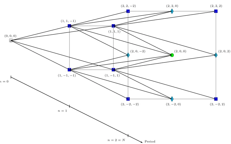
a) four extreme nodes, corresponding to the four possible combinations of

the extreme levels of the two state variables. These nodes, which are

referred to by (n, i, j), with i = _±n and j = _±n, can be reached by a

unique transitional path;

b) [(n + 1) ₋ 2] _× 4 external nodes, corresponding to all of the possible

to by (n, i, j), with either i = _±n and _|j_{| ≤} n ₋2 or _|i_{| ≤} n₋2 and

j =_±n, can be reached by two transitional paths;

c) [(n+1)₋2]2_{internal nodes, corresponding to all the possible combinations}

of the intermediate levels for both state variables. These nodes, which are

referred to by (n, i, j), with _|i_{| ≤} n₋2 and _|j_{| ≤}n₋2, can be reached

by four transitional paths.

Figure 1 illustrates the nodes and the transitional paths in a BB tree with

N = 2 periods.

[Figure 1 about here]

Let X(n, i, j) and r(n, j) be, respectively, the real estate asset value and

the (annualized) one-period short rate at node (n, i, j) of the bidimensional

binomial lattice. Furthermore, let puu(n, j), pud(n, j), pdu(n, j) and pdd(n, j) denote the joint probabilities of the up and down movements for the BB tree

at node (n, i, j) and as functions of the corresponding short rate r(n, j).

As it is shown in Figure 2, there are four branches emerging from the node (n, i, j) to represent the four possible combinations of the two state variables

going up or down at time step n+ 1. While the short (∆t-period) rate r(n, j)

can evolves either to a down-state, i.e.

r(n+ 1, j₋1), with probabilitypud(n, j) +pdd(n, j) = qr,

or to an up-state, i.e.

r(n+ 1, j+ 1), with probabilitypuu(n, j) +pdu(n, j) = pr,

the real estate asset valueX(n, i, j) rises or falls by an amount conditional on

the interest rate movements as follows



        

        

X(n+ 1, i+ 1, j+ 1), with probabilitypuu(n, j)

X(n+ 1, i+ 1, j₋1), with probabilitypud(n, j)

X(n+ 1, i₋1, j+ 1), with probabilitypdu(n, j)

X(n+ 1, i₋1, j₋1), with probabilitypdd(n, j)

Hence X(n + 1, i+ 1, j ₋ 1) and X(n + 1, i ₋1, j ₋ 1) represent up and

down values conditional on a downward movement of the short rate, while

X(n + 1, i + 1, j + 1) and X(n + 1, i ₋ 1, j + 1) are up and down values

equations (2.18)-(2.21) with the drift term ν(t) approximated now by

ν(n, j) = µ

r(n, j)₋δ₋ 1

2σ

2

X

¶

.

The recombining BB lattice can be constructed efficiently, extending the technique of forward induction first introduced by [7]. The procedure is an im-plementation of the binomial formulation of the Fokker-Planck forward equa-tion and it is applicable to the general class of term structure models which is referred to as “Brownian-path independent” and that includes, among others, the BDT model.

[Figure 2 about here]

Following [7] in our two-factor pricing model the levels of the two state

variables at timet, i.e. the natural logarithm of the real estate asset valuey(t)

and the spot interest rate r(t), are given respectively by

y(t) = UX(t) +σXW˜₁(t), (3.1)

r(t) =Ur(t) exp

³

σr(t) ˜W₂(t)

´

, (3.2)

whereUX(t) is the mean of the normal distribution foryat timet,Ur(t) is the

median of the lognormal distribution forrat timet,σX andσr(t) are the levels

(in percentage terms) of the constant and time-dependent volatilities ofXand

r respectively, ˜W1(t) and ˜W2(t) are the levels of the two correlated standard

Wiener processes defined under the same risk-neutral probability measure Q.

While the termUX(t) is a known function of the time variablet, that is

UX(t) =y(0) +ν(t)t, (3.3)

wherey(0) := lnX(0), with X(0) the initial value of the real estate asset, the

two unknown time-dependent functions Ur(t) and σr(t) must be determined

at each time period in order to fit the model to the current market term struc-tures. If the model is implemented to fit just the interest rate term structure,

with σr(t) set equal to a constant level σr, we only have to determine the

medianUr(t) and thus the level of the spot interest rate is given by

r(t) =Ur(t) exp

³

σrW˜2(t) ´

. (3.4)

Since as ∆t _→ 0 the BB process ³i√∆t, j√∆t´ converges to the

bidi-mensional standard Wiener process³W˜1(t), W˜1(t) ´

X(n, i, j) = X(0) exp³i∆y(n, j)´, (3.5)

r(n, j) =Ur(n) exp

³

σr(n)j√∆t´, (3.6)

with _|i_{| ≤} n and _|j_{| ≤} n and where the equal jump size ∆y(n, j) for the

natural logarithm of the real estate asset value is defined by (2.15). To build

the recombining tree for the two state variables (i.e. determining X(n, i, j)

and r(n, j) for each time period n and levels i and j) therefore requires us to

determine Ur(n) and σr(n).

3.1 Determining the time-dependent functions Ur(t) and σ_r(t)

In order to determine the time-dependent functionsUr(t) andσr(t) we resort

to the forward induction technique which involves using the Arrow-Debreu securities. Let us assume to have a security which pays the following monetary

units _





1, if node (n, i, j) is reached

0, otherwise

and letA(n, i, j) denote the value at time 0 (i.e., at root node (0,0,0)) of this

Arrow-Debreu security that represents the building block of any security. In

particular, the price of a pure discount bond which matures at period n+ 1

can be written in terms of the Arrow-Debreu prices as follows

B(n+ 1) =X

i X

j

A(n, i, j)d(n, j), (3.7)

with the two summations that take place across all of the possible nodes at

period n, that is for _|i_{| ≤} n and _|j_{| ≤} n, and where d(n, j), which denotes

the price at periodn and state j of the zero-coupon bond maturing at period

n+ 1 (i.e. the one-period discount factor at nodes (n, i, j), for all_|i_{| ≤}n), can

be defined as follows

d(n, j) = 

   

   

1

1 +r(n, j)∆t, for simple compounding

exph₋r(n, j)∆ti, for continuous compounding

(3.8)

As pointed out by [8], the stability of lognormal short rate models is ensured by using the simple or effective annual rates instead of the continuously com-pounding interest rates.

at period n, level i for the variable X and level j for the variabile r (i.e., the

A(n, i, j)’s), can be computed from the known values at period n₋1 taking

into account all possibile transitional paths that lead into node (n, i, j).

Firstly, each of the four extreme nodes at period n, with n = 1, 2. . . , N,

can be reached by a unique path and thus the Arrow-Debreu prices satisfy the following recursive relation

A(n, i, j) =                                           

pud(n₋1, j+ 1)A(n₋1, i₋1, j+ 1)d(n₋1, j+ 1), i=n, j=₋n puu(n₋1, j ₋1)A(n₋1, i₋1, j₋1)d(n₋1, j₋1),

i=n, j=n

pdd(n₋1, j+ 1)A(n₋1, i+ 1, j+ 1)d(n₋1, j+ 1), i=₋n, j=₋n pdu(n₋1, j₋1)A(n₋1, i+ 1, j₋1)d(n₋1, j₋1),

i=₋n, j=n

(3.9)

that is, we multiply each transitional probability by its state-contingent price

at previous period n₋1 and the corresponding one-period discount factor.

For each of the [(n+ 1)₋2]_×4 external nodes there are two transitional

paths to be considered and therefore the Arrow-Debreu prices for such nodes

at period n are computed recursively according to the following equation

A(n, i, j) =                                                                           

puu(n₋1, j ₋1)A(n₋1, i₋1, j₋1)d(n₋1, j₋1) +pud(n₋1, j+ 1)A(n₋1, i₋1, j+ 1)d(n₋1, j+ 1),

i=n, _|j_{| ≤}n₋2

pdd(n₋1, j+ 1)A(n₋1, i+ 1, j+ 1)d(n₋1, j+ 1) +pdu(n₋1, j₋1)A(n₋1, i+ 1, j₋1)d(n₋1, j₋1),

i=₋n, _|j_{| ≤}n₋2

pdd(n₋1, j+ 1)A(n₋1, i+ 1, j+ 1)d(n₋1, j+ 1) +pud(n₋1, j+ 1)A(n₋1, i₋1, j+ 1)d(n₋1, j+ 1),

|i_{| ≤}n₋2, j =₋n

puu(n₋1, j ₋1)A(n₋1, i₋1, j₋1)d(n₋1, j₋1) +pdu(n−1, j−1)A(n−1, i+ 1, j−1)d(n−1, j−1),

|i_{| ≤}n₋2, j =n

that is, for each pair of nodes that lead into (n, i, j) we sum the two

state-contingent prices at previous period n₋1, multiplied by their corresponding

probabilities and one-period discount factors.

Finally, for each of the [(n + 1) ₋2]2 _{internal nodes, the Arrow-Debreu}

prices at period n satisfy the following equation

A(n, i, j) =pdu(n₋1, j ₋1)A(n₋1, i+ 1, j ₋1)d(n₋1, j₋1) +pdd(n₋1, j+ 1)A(n₋1, i+ 1, j+ 1)d(n₋1, j+ 1)

+puu(n₋1, j₋1)A(n₋1, i₋1, j₋1)d(n₋1, j₋1) (3.11) +pud(n−1, j+ 1)A(n−1, i−1, j+ 1)d(n−1, j+ 1),

|i_{| ≤}n₋2, _|j_{| ≤}n₋2,

that shows the four possibile transitional paths through which the internal

node (n, i, j) can be reached moving on the BB lattice from the previous

period n₋1. Note that the Arrow-Debreu price at the initial period n = 0

and level 0 for both state variables, i.e., the initial condition for the recursive

procedure, is by definition given by A(0,0,0) = 1.

Before describing the general procedure to implement and calibrate the BB lattice so that it is consistent with the current interest rate and volatility term structures, in the next section we show how a version of the BB tree fitted to the yield curve only can be efficiently constructed.

3.2 Fitting the yield curve only

Many practitioners when using the BDT model, set the volatility functionσr(t)

to a constant level σr and so only fit to the yield curve. It follows that the

mean-reverting term within the drift function ψ(t) equates to zero, and then

the spot rate process is described by the SDE (2.3) whereas its discrete-time representation is given by

r(n, j) =Ur(n) exp

³

σrj

√

∆t´, _|j_{| ≤}n. (3.12)

Using equations (3.12) and (3.7) and simple compounding for the one-period

discount factor d(n, j) as expressed by equation (3.8), the price of the pure

discount bond maturing at periodn+ 1 can be rewritten as

B(n+ 1) =X

i X

j

A(n, i, j) 1 1 +Ur(n) exp

³

σrj

√

Given that the discount function d(n, j) is determined by the market data,

the only unknown in equation (3.13) is the medianUr(n) of the lognormal

dis-tribution forrat periodn. Due to the analytical intractability of the lognormal

models, we cannot rearrange equation (3.13) to obtain Ur(n) explicitly, and

then we need to use a suitable numerical search technique. In order to solve

numerically equation (3.13) and then get an approximated value forUr(n), by

which to determine the short rate at periodnusing equation (3.12), we resort

to the Newton-Raphson method.

Let n_≥1 and assume thatUr(n−1), A(n−1, i, j),r(n−1, j),d(n−1, j)

and _{puu(n₋1, j), pud(n₋1, j), pdu(n₋1, j), pdd(n₋1, j)_}have been found

for all states iandj at periodn₋1. The values at the initial time, i.e. period

n = 0, are Ur(0) = r(0,0) =Y(1), A(0,0,0) = 1, d(0,0) = 1/(1 +r(0,0) ∆t).

The procedure can be summarized by the following steps:

Step1: From the initial yield curve, compute the market price of then-period

pure discount bond ˆB(n), for n= 1, 2 . . . , N+ 1;

Step 2: Using recursive forward equations (3.9)–(3.11) relative to the three

types of nodes, generate the Arrow-Debreu prices A(n, i, j), for _|i_{| ≤}n and

|j_{| ≤}n, with n_≤N;

Step 3: For n _≤ N, substitute ˆB(n+ 1) into nonlinear equation (3.13) and

solve it for the only unknown Ur(n) by using Newton-Raphson method;

Step 4: From Ur(n) calculate r(n, j) and d(n, j), for |j| ≤ n, with n ≤ N,

using equations (3.12) and (3.8), respectively;

Step 5: From r(n, j), with _|j_{| ≤}n, compute the joint probabilitiespuu(n, j),

pud(n, j), pdu(n, j) and pdd(n, j) by equations (2.18)–(2.21) and calculate

X(n, i, j) by equation (3.5), for_|i_{| ≤}n, withn _≤N.

3.3 Fitting interest rate and volatility term structures

In this section we present the implementation procedure of the BB tree in its full generality. In order to fit the tree to both interest rate and volatility term structures we must consider the discrete-time equivalent of the spot rate process as expressed in equation (3.6).

LetBU U(n),BDU(n),BU D(n), andBDD(n) denote the four possibile prices at

period 1 of a pure discount bond maturing at periodn, withn = 1, 2, . . . , N+

1, andYU U(n),YDU(n),YU D(n), andYDD(n) be the corresponding yields. Given

that at period 1 there are only two different realizations for the short (∆t

-period) rate, r(1,₋1) and r(1,1), it implies that BU U(n) = BDU(n) ≡ BU(n)

and BU D(n) = BDD(n) ≡ BD(n). Consequently, we have only two possibile

yields,YU(n)≡YU U(n) =YDU(n) andYD(n)≡YU D(n) = YDD(n). Since upward

and downward moves of the short rate differ by the factor exph2σY(n)

√

∆ti

YU(n)

YD(n)

= exph2σY(n)

√

∆ti. (3.14)

where σY(n) denote the initial volatility corresponding to the yield on a pure

discount bond which matures at period n _≥ 1. Recalling the two possible

ways to define the relationship between the initial price B(0, n) _≡ B(n) and

the corresponding yield Y(0, n) _≡Y(n) of a n-maturity pure discount bond,

that is

B(n) = 

    

    

1 h

1 +Y(n)∆tin, for simple compounding

exph₋Y(n)n∆ti, for continuous compounding

(3.15)

we can solve for the initial yield volatilityσY(n) in equations (3.14) to obtain

the following formula

σY(n) =

1 2√∆t ln

Ã

YU(n)

YD(n)

!

. (3.16)

The two different discount functions BU(n) and BD(n), for n ≥ 2, are in

relation to the prices at the initial time of n-maturity pure discount bonds,

B(n), according the following discounted expectation formula

B(n) = 1 1 +r(0,0)∆t

·

BU(n)

³

puu(0,0) +pdu(0,0)´

+BD(n)

³

pud(0,0) +pdd(0,0)´ ¸

. (3.17)

Using the probability conditions (2.13)–(2.14) and the continuous compound-ing as expressed in equation (3.15), we solve simultaneously equations (3.16) and (3.17) and find the following system of nonlinear equations



 

 

BD(n) =BU(n)

exp[−2σY(n)

√ ∆t]

BU(n) +BU(n)

exp[−2σY(n)

√

∆t] = 2_B(n)h

1 +r(0,0)∆ti

(3.18)

In order to determine the time-dependent functions that match the yield and volatility curves we use the forward induction technique which now in-volves defining the Arrow-Debreu securities as seen from the four possibile nodes at period 1. The following notation is then required:

AU U(n, i, j): Arrow-Debreu price at node (1,1,1) of a security that pays

ADU(n, i, j): Arrow-Debreu price at node (1,−1,1) of a security that pays

off 1 if states iand j are realized at periodn and 0 otherwise;

AU D(n, i, j): Arrow-Debreu price at node (1,1,−1) of a security that pays

off 1 if states iand j are realized at periodn and 0 otherwise;

ADD(n, i, j): Arrow-Debreu price at node (1,−1,−1) of a security that

pays off 1 if states iand j are realized at periodn and 0 otherwise.

Note thatAU U(n, i, j) =ADU(n, i−2, j) andAU D(n, i, j) =ADD(n, i−2, j), for

|i_{| ≤}n. It follows that the initial condition for the recursive condition is then

given by AU U(1,1,1) = AU U(1,−1,1) = 1 and AU D(1,1,1) =ADD(1,−1,1) =

1. Therefore, the prices at period 1 of (n+ 1)-maturity pure discount bonds,

i.e. BU(n+ 1) and BD(n+ 1), for n= 1, 2, . . . , N, can be written in terms of

the newly defined Arrow-Debreu prices in the two equivalent forms as follows

BU(n+ 1)≡

                      

BU U(n+ 1) =

X

i X

j

AU U(n, i, j)d(n, j),

at node (1,1,1)

BDU(n+ 1) =

X

i X

j

ADU(n, i, j)d(n, j),

at node (1,₋1,1)

(3.19)

BD(n+ 1)≡

                      

BU D(n+ 1) =

X

i X

j

AU D(n, i, j)d(n, j),

at node (1,1,₋1)

BDD(n+ 1) =

X

i X

j

ADD(n, i, j)d(n, j),

at node (1,₋1,₋1)

(3.20)

where the one-period discount factor,d(n, j), is defined using the simple

com-pounding formula given in equation (3.8), that is

d(n, j) = 1

1 +r(n, j)∆t =

1 1 +Ur(n) exp

³

σr(n)j

√

∆t´∆t.

Given that the term structure of pure discount bond prices and the term structure of yield volatilities, i.e. ˆB(n) and ˆσY(n) for n ≥1, are known at the

initial time from market data, we are able to find the two discount functions,

BU(n) andBD(n) for each periodn ≥1, by using the system of nonlinear

two unknowns, Ur(n) and σr(n), to be solved simultaneously. Note that the

prices AU U(n, i, j), ADU(n, i, j), AU D(n, i, j) and ADD(n, i, j) of the newly

de-fined Arrow-Debreu securities are updated according to the three types of node (i.e. extreme, external or internal) using recursive relations analogous to equations (3.9)–(3.11).

Let n_≥1 and assume that Ur(n−1), σr(n−1), AU U(n−1, i, j),ADU(n−

1, i, j), AU D(n−1, i, j) ADD(n−1, i, j), r(n−1, j), d(n−1, j) and {puu(n−

1, j), pud(n−1, j), pdu(n−1, j), pdd(n−1, j)} have been found for all states

i and j at period n₋1. The values at the initial time are Ur(0) = r(0,0) =

Y(1), AU U(1,1,1) = ADU(1,−1,1) = 1, AU D(1,1,−1) = ADD(1,−1,−1) = 1,

σr(0) =σY(1) and d(0,0) = 1/(1 +r(0,0) ∆t). The procedure consists of the

following steps:

Step1: From the initial yield and volatility curves, compute the market price

and the corresponding yield volatility of the n-period pure discount bond,

i.e. ˆB(n) and ˆσY(n), for each period n≥1;

Step2: Substitute ˆB(n) and ˆσY(n) into system of nonlinear equation (3.18) to

deriveBU(n) and consequentlyBD(n), forn≥2, by using Newton-Raphson

iteration technique;

Step 3: Using recursive forward relations analogous to equations (3.9)–(3.11)

for three types of nodes, generate the Arrow-Debreu prices AU U(n, i, j),

ADU(n, i, j), AU D(n, i, j) and ADD(n, i, j), for |i| ≤n and |j| ≤n;

Step 4: Substitute BU(n+ 1) andBD(n+ 1) into nonlinear equations (3.19)–

(3.20) and solve them for the two unknowns Ur(n) andσr(n) by using

bidi-mensional Newton-Raphson method;

Step 5: FromUr(n) andσr(n) calculater(n, j) andd(n, j), for|j| ≤n, using

equations (3.6) and (3.8), respectively;

Step 6: From r(n, j), with _|j_{| ≤} n, compute the probabilities puu(n, j),

pud(n, j), pdu(n, j) and pdd(n, j) by equations (2.18)–(2.21) and calculate

X(n, i, j) by equation (3.5), for_|i_{| ≤}n.

4 An application to European and American options

An attractive feature of the BB lattice framework presented in this paper lies in the fact that, once the tree is built, any security dependent upon the two state variables can be easily evaluated by backward induction.

Let Π(n, i, j) be the value of a real estate derivative at time step n < N,

at level i in the underlying real estate asset value and at level j in the short

rate. Within our two-factor pricing model, the value Π(n, i, j) of the derivative

security is obtained as the discounted present value of the four possible future

Π(n, i, j) =d(n, j)hΠ(n+ 1, i+ 1, j₋1)pud(n, j) + Π(n+ 1, i₋1, j₋1)pdd(n, j) + Π(n+ 1, i+ 1, j+ 1)puu(n, j)

+ Π(n+ 1, i₋1, j+ 1)pdu(n, j)i, (4.1)

where the one-period discount factord(n, j) is defined by (3.8). This iteration

continues backward all the way to the initial time n = 0. The initial value of

the derivative security is then given by Π0 ≡Π(0,0,0).

The pricing problem of any contingent claim dependent upon the two state variables can be solved using the same general backward iteration procedure, but the distinctive features that characterize a specific derivative contract are entirely embodied in the terminal and boundary conditions that, therefore, must be appropriately defined before solving the valuation problem.

As an application of the BB lattice framework introduced in this paper

we consider the pricing problem at time t0 ≥ 0 of European and American

options written on a real estate asset whose value processX follows (2.1) and

with payoff at time T (i.e. terminal condition) given by

H(T) = 

  

   ³

X(T)₋K´+, for a call option

³

K₋X(T)´+, for a put option

where (x)+ _{= max(x,0), T ≥ t}

0 is the maturity date and K ≥0 is the strike

price of the option. Let VE(n, i, j) and VA(n, i, j) denote the value at node

(n, i, j), for n = 0, 1, . . . , N and _|i_|,_|j_{| ≤} n, of the European and American option, respectively. Using a calibrated BB tree with the life of the option

τ :=T ₋t0 divides into N equal time periods (or steps) of length ∆t=τ /N

years, the values of the European and American options at the maturity date

T, i.e. at the N-th time period, are determined by the corresponding payoff

as follows

Π(N, i, j)_≡H(N, i, j) = 

  

   ³

X(N, i, j)₋K´+, for a call option

³

K₋X(N, i, j)´+, for a put option (4.2)

whereX(N, i, j) =X(t0) exp ³

i∆y(N, j)´, for _|i_|,_|j_{| ≤}N, are all of the

possi-ble values of the real estate asset at the final period N relative to the initial

valueX(t0) and to the possible realizations of the short rater(N, i, j) by which

is determined the drift term for ∆y(N, j).

As we have shown above the value of the derivative at any node (n, i, j),

withn < N, in the recombining tree is related to the four connecting nodes at

the following time period n+ 1 according to the general discounted

procedure only has to be performed as far back as time period N when the terminal condition of the option (4.2) is implemented. Hence the European

option value at node (n, i, j) is given by

VE(n, i, j) = Π(n, i, j), ∀i, j at period n < N . (4.3)

For American options, in order to evaluate the possibility of early exercise when applying the backward induction procedure by equation (4.1), we need to take the maximum of the discounted expectation and the intrinsic value (i.e. boundary conditions) of the option at each node. Similarly, after that the terminal condition of the option (4.2) has been implemented, the American

option value at node (n, i, j), for all i,j at period n < N, is then given by

VA(n, i, j) =



  

   h

Π(n, i, j), ³X(n, i, j)₋K´i+, for a call option

h

Π(n, i, j), ³K ₋X(n, i, j)´i+, for a put option

(4.4)

4.1 Numerical results and discussion

Once the branching process with both jump sizes and joint probabilities are correctly determined in such way that the resulting BB tree is consistent with market data, the general backward recursive procedure along with the appropriate terminal and boundary conditions allow us to value any specific contingent claim dependent upon the two state variables.

The numerical results reported in Table 1 show how the standard BSM model can be successfully recovered by implementing a BB lattice consistent with a flat yield curve and with yield volatilities and correlation coefficient set

to be zero2_{. European and American options written on a real estate asset}

without any income flow, i.e. δ = 0, are used for this purpose. The value

at initial time t0 = 0 of the underlying asset, X(0), is 95, 100 or 110, the

strike price,K, is 100, the time of maturity, T, is six months or one year, the

instantaneous volatility of the percentage change in real estate asset value,σX,

is of 20 or 30 per cent per annum and the risk-free interest rate,r:=r(t0, T), is

5 per cent per annum. We assume that the two state variables are uncorrelated while the yield curve is flat at 5 per cent and the spot rate volatility is equal

to zero, that isρ(t)_≡0,r(t)_≡randσr(t)≡0,∀t≥0. To implement the BB

tree we use a number of time periods,N, that ranges from 20 to 240 while the

analytic solution is calculated using the standard BSM pricing formula. The Crank-Nicolson finite difference (CNFD) method with a number of time steps equals to 1500 and 3000 for six-months and one-year options, respectively, is

used to price the American put options since in the absence of income flows there is the usual equivalence between American and European calls.

[Table 1 about here]

From the results in Table 1, it is clear that the option prices obtained by the BB model converge with a slightly oscillatory behavior to both analytical and numerical solutions for any given value of the model parameters. Be-sides demonstrating numerical convergence to the BSM model and the CNFD method, an important analytical remark on the features of the two-factor pricing model when the spot interest rate is assumed constant may be useful to be considered. In fact in the special case of constant volatility structure, the two-factor pricing model is described by the following continuous-time risk-neutralized SDEs:

dlnX(t) =ν(t)dt + σXdW˜1(t),

dlnr(t) = ∂lnu(t)

∂t dt + σrdW˜2(t).

where corr(dW˜1(t), dW˜2(t)) = ρ(t) and u(t) is the median of the spot rate

distribution at time t_≥0.

When we assume that the two state variables X and r are uncorrelated

and the initial yield curve is flat with the spot rate volatility equals zero, the

diffusion process forr reduces to an ordinary differential equation of the form

dlnr(t) = 0. This result along with the initial conditionr(t0) =r implies that

the spot interest rate is a constant function, i.e.

r(t) =r, _∀t _≥0 and r _∈R+_,

which gives the drift term for dlnX(t) to be constant, that is ν(t) _≡ ν :=

(r₋δ₋1 2 σ

2

X). It follows that the jump sizes for lnrare equal to zero and then

the BB lattice used to approximate the continuous-time diffusion processes reduces to a standard univariate binomial tree with time-invariant risk-neutral probabilities and additive jumps. More specifically, from the system consisting of equations (2.6)-(2.7) and (2.11)-(2.14) it turns out that the equal jump size

and the unconditional probabilities of upward and downward jumps for lnX

are respectively given by

∆y(t) =qσ2

X∆t+ν2∆t2 := ∆y, (4.5)

puu(t) +pud(t) =1

2+

1 2

ν∆t

∆y := pX, (4.6)

pdu(t) +pdd(t) =1

2−

1 2

ν∆t

∆y = 1−pX := qX. (4.7)

Note that in this particular formulation of the BB model we cannot ob-tain separately each of the joint probabilities,puu(t), pud(t),pdu(t) andpdd(t), by solving the system of equations (2.6)-(2.7) and (2.11)-(2.14). Hence the BB lattice collapses into a standard binomial tree in which the equal jump size (4.5) and the risk-neutral probabilities (4.6)-(4.7) are identical to those of the binomial model originally developed by [5].

In order to assess the general validity of the BB model, we must take into consideration a stochastic interest rate and then fit the BB lattice to the initial yield and volatility curves. To simplify the analysis throughout this section, we assume that the volatility term structure is constant at level of 5 per cent

per annum, i.e. σr(t) ≡ 0.05 ∀t ≥ 0, while the term structure of interest

rates can be rising or declining according to the behavior described by the

respective initial yield curve. Let us consider a time horizonT of one year and

divide it into NT = 20 periods, each having length ∆T := 1/NT = 0.05 years.

Assuming that the yield on pure discount bond maturing at the end of the

first time interval ∆T is equal to 5 per cent per annum, we build the BB tree

consistent with the following two different interest rate term structures:

(a) Increasing initial yield curve: the interest rate increases from 5 per cent

after ∆T years to 6 per cent afterNT·∆T = 1 year and remains constant

during each time interval of size ∆T;

(b) Decreasing initial yield curve: the interest rate decreases from 5 per cent

after ∆T years to 4 per cent afterNT·∆T = 1 year and remains constant

during each time interval of size ∆T.

Since the surface of the option value obtained under the BB model is con-sistent with that calculated using the standard BSM pricing formula, we take a closer look at what are the patterns of the differences of European option values with stochastic interest rate minus the option values with constant in-terest rate. To calculate the surface of these differences over time to maturity and across different moneyness we use for common parameters of the two

models the following values: K = 100, r = 0.05, δ = 0, σX = 0.2, ρ(t) ≡ 0

∀t _≥ 0, with X(t0) ranges from 90 to 110, and time to maturity τ = ¯T −t0

from 0 to 1 year. To ensure that option prices with different maturities are

broadly comparable, the number of periods N in which is divided the time

horizon of the option varies such that the length ∆t of each period is equal

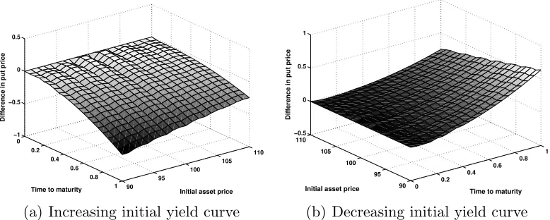
can see from Figures 3(a) and 4(a), when the term structure is rising, then the constant-rate model systematically underprices European calls and over-prices European puts with respect to the stochastic-rate model. The degree of mispricing increases proportionately with the time to maturity and the abso-lute moneyness. The findings are just the opposite when the term structure is falling, as shown in Figures 3(b) and 4(b). The constant-rate model overprices European calls and underprices European puts with the mispricing that is largest for long time-to-maturity and in-the-money options.

[Figure 3 about here]

[Figure 4 about here]

When taking non-zero correlation coefficient into consideration, the mag-nitude of differences between option prices under stochastic-rate using the BB lattice and those calculated by the BSM pricing formula with constant-rate can exhibit some interesting patterns. Tables 2 and 3 report and compare prices and percentage pricing differences of European calls and puts

respec-tively, under different constant levels of the correlation coefficient ρ and over

several times of maturity and moneyness levels. As previously we use for

com-mon parameters the following values: K = 100,δ = 0, r= 0.05 and σX = 0.2.

The BB tree is fitted to the two different initial yield curves with constant

spot rate volatility of 0.05 and using a number of periods N that varies such

that the length ∆t of each time step is equal to 0.005.

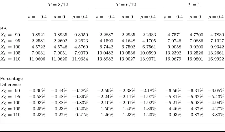
Table 2 shows that the BSM model underprices European calls when the initial yield curve has an upward slope and overprices European calls when the initial yield curve has a downward slope. As the time of maturity in-creases, the percentage pricing errors increases almost proportionately in ab-solute value. Table 2 reveals that, except for short-maturity options (three months), the absolute-percentage pricing error of out-of-the money call (i.e.,

X0 < K) is largest compared to at-the-money and in-the-money calls (i.e.,

X0 ≥ K). Specifically, percentage differences for medium- and long-maturity

call options (six months and one year) are decreasing functions of the

mon-eyness level. Finally, comparison of percentage differences across the several ρ

values reveals that the degree of mispricing increases as the correlation

coef-ficient ρ ranges from -0.4 to 0.4 when the term structure is rising, while the

pricing error decreases as ρ varies from negative to positive values when the

term structure is falling.

[Table 2 about here]

Table 3 shows that for European puts the sign of the percentage pricing dif-ferences under stochastic- and constant-rate using respectively BB and BSM models is opposite to that of the European calls. Specifically, when the initial yield curve is upward sloping European puts turn out to be overvalued by the BSM model, while it undervalues European puts when the initial yield curve is downward sloping. Similarly, longer maturity implies larger effects of mispricing and, except for three-months options, as the moneyness level decreases the percentage differences in absolute terms increases. Finally, the effect of the correlation coefficient on the relative magnitude of pricing errors is the same as for European calls regarding to the direction of mispricing.

Hence, the absolute-percentage differences decreases as ρ ranges from -0.4 to

0.4 when the option is underpriced (i.e. when the term structure is rising),

while percentage differences increases as ρ varies from negative to positive

values when the option is overpriced (i.e. when the term structure is falling). Although we have shown graphically and numerically the effects of stochas-tic interest rate only on European call and put options, it is easy to verify that the obtained results are valid for both European and American options writ-ten on real estate assets without income flow or with constant continuously paid cash-flow.

5 Conclusions

In this paper, we develop a two-factor model that is both computationally efficient and numerically accurate for pricing the growing class of interest rate sensitive real estate derivatives. The kernel of the model is made of a spot rate process with drift and volatility terms consistent with the current market term structures and a possibly correlated underlying real estate value process. These diffusion processes are approximated in discrete-time by a bidimen-sional binomial (BB) model. An analytical solution for jumps measure and risk-neutral probabilities are derived with the attractive property to avoid the negative-probability problem. The calibration procedure to market data is based on the forward induction technique which involves using the Arrow-Debreu securities.

References

[1] F. Black, M. Scholes, The pricing of options and corporate liabilities.Journal of Political Economy 81_{637-654 (1973).}

[2] R. Merton, Theory of rational option pricing. Bell Journal of Economics and Management Science 4 _{141-183 (1973).}

[3] F. Black, E. Derman, W. Toy, A one-factor model of interest rates and its applications to treasury bond options. Financial Analysts Journal 46 _33-39

(1990).

[4] R. Buttimer, J. Kau, C. Slawson, A model for securities dependent upon a real estate index.Journal of Housing Economics 6 _{16-30 (1997).}

[5] L. Trigeorgis, A log-transformed binomial numerical analysis method for valuing complex multi-option investments. Journal of Financial and Quantitative Analysis 26 _{309-326 (1991).}

[6] J. Cox, S. Ross, M. Rubinstein, Option pricing: a simplified approach.Journal of Financial Economics 7_{229-263 (1979).}

[7] F. Jamshidian, Forward induction and construction of yield curve diffusion models.Journal of Fixed Income 1 _{62-74 (1991).}

[8] K. Sandmann, D. Sondermann, A note on the stability of lognormal interest rate models and the pricing of Eurodollar futures.Mathematical Finance 7 _119-125

r s

+

(0,0,0)

n= 0

r s

(1,1,−1)

r s

(1,−1,−1)

r s

(1,−1,1)

r s

(1,1,1)

n= 1

r s

(2,2,−2)

l d

(2,2,0)

r s

(2,2,2)

l

d(2,0,−2) bc(2,0,0) ld(2,0,2)

r s

(2,−2,−2)

l d

(2,−2,0)

r s

(2,−2,2)

n= 2 =N

r s

+ Root node

r

sExtreme node

l

dExternal node

b

cInternal node

Period

Fig. 1. Bidimensional binomial tree withN = 2 periods.

r s

r s

r

s rs

r s

Period n

n+ 1 pud(n, j)

puu(n, j)

pdd(n, j) pdu(n, j)

r(n, j)

X(n, i, j)

r(n+ 1, j−1)

X(n+ 1, i+ 1, j−1)

r(n+ 1, j+ 1)

X(n+ 1, i+ 1, j+ 1)

r(n+ 1, j−1)

X(n+ 1, i−1, j−1)

r(n+ 1, j+ 1)

X(n+ 1, i−1, j+ 1)

Table 1

Convergence to BSM model and CNFM method of European and American Vanilla Options under the BB model

No of periods T = 6 months T = 1 year

σX= 0.2 σX= 0.3 σX = 0.2 σX= 0.3

X0= 95 X0= 100 X0= 105 X0= 95 X0= 100 X0= 105 X0= 95 X0= 100 X0= 105 X0= 95 X0= 100 X0= 105

European call (American call)

20 4.2642 6.8197 10.2295 7.0222 9.5300 12.8970 7.5923 10.3537 13.9438 11.3880 14.0824 17.6148 40 4.2508 6.8541 10.1893 6.9478 9.5823 12.8281 7.5169 10.4020 13.8767 11.3374 14.1566 17.5720 60 4.2728 6.8656 10.2166 6.9088 9.5998 12.7910 7.4780 10.4182 13.8407 11.3067 14.1814 17.5440 80 4.2676 6.8714 10.2164 6.9165 9.6085 12.7783 7.5086 10.4263 13.8495 11.2860 14.1939 17.5246 100 4.2562 6.8748 10.2088 6.9333 9.6138 12.7981 7.5207 10.4311 13.8636 11.2709 14.2013 17.5103 120 4.2435 6.8772 10.1991 6.9397 9.6173 12.8069 7.5239 10.4344 13.8688 11.2592 14.2063 17.4991 160 4.2591 6.8800 10.2024 6.9399 9.6217 12.8105 7.5201 10.4384 13.8685 11.2649 14.2125 17.4906 200 4.2603 6.8818 10.2071 6.9341 9.6243 12.8071 7.5120 10.4408 13.8631 11.2767 14.2163 17.5045 240 4.2553 6.8829 10.2052 6.9268 9.6261 12.8015 7.5031 10.4425 13.8563 11.2812 14.2188 17.5107 BSM formula 4_.2545 6_.8887 10_.2013 6_.9282 9_.6349 12_.7986 7_.5109 10_.4506 13_.8579 11_.2733 14_.2313 17_.5051

European put

20 6.7959 4.3513 2.7612 9.5541 7.0620 5.4291 7.7178 5.4793 4.0695 11.5148 9.2095 7.7421 40 6.7821 4.3854 2.7206 9.4792 7.1138 5.3596 7.6411 5.5263 4.0011 11.4623 9.2816 7.6971 60 6.8040 4.3968 2.7479 9.4401 7.1311 5.3223 7.6018 5.5420 3.9646 11.4309 9.3057 7.6684 80 6.7988 4.4025 2.7476 9.4477 7.1398 5.3096 7.6321 5.5499 3.9732 11.4099 9.3178 7.6486 100 6.7873 4.4060 2.7399 9.4645 7.1450 5.3293 7.6441 5.5546 3.9871 11.3946 9.3251 7.6341 120 6.7746 4.4083 2.7302 9.4709 7.1485 5.3381 7.6473 5.5577 3.9922 11.3828 9.3299 7.6227 160 6.7902 4.4111 2.7335 9.4710 7.1528 5.3417 7.6434 5.5617 3.9918 11.3883 9.3360 7.6141 200 6.7914 4.4128 2.7382 9.4652 7.1554 5.3382 7.6351 5.5641 3.9863 11.4001 9.3396 7.6279 240 6.7864 4.4140 2.7362 9.4578 7.1572 5.3326 7.6262 5.5656 3.9794 11.4045 9.3421 7.6340 BSM formula 6_.7855 4_.4197 2_.7322 9_.4592 7_.1659 5_.3295 7_.6338 5_.5735 3_.9808 11_.3963 9_.3542 7_.6280

American put

20 7.2289 4.6240 2.8942 9.8893 7.3361 5.5807 8.5044 6.0522 4.3813 12.2017 9.7992 8.1089 40 7.2320 4.6400 2.8459 9.8190 7.3656 5.5184 8.4544 6.0722 4.3305 12.1431 9.8351 8.0787 60 7.2409 4.6454 2.8688 9.7894 7.3749 5.4833 8.4398 6.0780 4.3008 12.1145 9.8470 8.0552 80 7.2347 4.6480 2.8700 9.7988 7.3799 5.4673 8.4562 6.0814 4.2998 12.0982 9.8529 8.0386 100 7.2262 4.6495 2.8641 9.8101 7.3828 5.4820 8.4611 6.0833 4.3094 12.0871 9.8562 8.0260 120 7.2194 4.6505 2.8561 9.8135 7.3847 5.4896 8.4617 6.0845 4.3136 12.0795 9.8585 8.0160 160 7.2290 4.6519 2.8565 9.8118 7.3870 5.4931 8.4577 6.0860 4.3142 12.0856 9.8616 8.0057 200 7.2287 4.6527 2.8606 9.8063 7.3884 5.4904 8.4525 6.0869 4.3105 12.0927 9.8633 8.0148 240 7.2250 4.6532 2.8593 9.8003 7.3894 5.4855 8.4483 6.0874 4.3055 12.0948 9.8645 8.0196 CNFD method 7_.2224 4_.6539 2_.8542 9_.7990 7_.3915 5_.4793 8_.4499 6_.0891 4_.3038 12_.0852 9_.8682 8_.0125

This table reports prices at initial timet0= 0 for European and American calls and puts under constant-rate assumption calculated using the BSM model and the BB model. The initial value of the underlying asset (X0) is 95, 100 or 105, the strike price (K) is 100, the time of maturity (T) is 6 months or 1 year, the instantaneous volatility of the percentage change in real estate asset value (σ ) is 0.2 or 0.3 per annum, the continuously paid cash-flow (δ) is 0, the risk-free interest rate (r) is 0.05 per annum, the yield

0 0.2 0.4 0.6 0.8 1 90 95 100 105 110 −0.5 0 0.5 1

Time to maturity Initial asset price

Difference in call price

(a) Increasing initial yield curve

0 0.2 0.4 0.6 0.8 1 90 95 100 105 110 −1 −0.5 0 0.5

Initial asset price Time to maturity

Difference in call price

(b) Decreasing initial yield curve

Fig. 3. Effects of stochastic interest rate in pricing European calls.

The left and right graphs of this figure show the pricing differences for European calls under stochastic-rate assumption using the BB model and within the standard BSM model with constant-rate, distinguishing between increasing and decreasing initial yield curves. To determine the surfaces, option prices are cal-culated for different moneyness levels choosing the initial value of the underlying asset (X0) from 90 to

110 and for different times to maturity (τ) from 0 to 1 year. Values chosen for common parameters are K= 100,r= 0.05,δ= 0,σX= 0.2,ρ(t)≡0,∀t≥0. The BB lattice is fitted to the two different initial

yield curves with constant spot rate volatility (σr) of 0.05 and using a number of periods (N) that varies

such that the length ∆tof each time step is of 0.00625.

0 0.2 0.4 0.6 0.8 1 90 95 100 105 110 −1 −0.5 0 0.5

Initial asset price Time to maturity

Difference in put price

(a) Increasing initial yield curve

0 0.2 0.4 0.6 0.8 1 90 95 100 105 110 −0.5 0 0.5 1

Time to maturity Initial asset price

Difference in put price

(b) Decreasing initial yield curve

Fig. 4. Effects of stochastic interest rate in pricing European puts.

The left and right graphs of this figure show the pricing differences for European puts under stochastic-rate assumption using the BB model and within the standard BSM model with constant-rate, distinguishing between increasing and decreasing initial yield curves. To determine the surfaces, option prices are cal-culated for different moneyness levels choosing the initial value of the underlying asset (X0) from 90 to

110 and for different times to maturity (τ) from 0 to 1 year. Values chosen for common parameters are K= 100,r= 0.05,δ= 0,σX= 0.2,ρ(t)≡0,∀t≥0. The BB lattice is fitted to the two different initial

yield curves with constant spot rate volatility (σr) of 0.05 and using a number of periods (N) that varies

Table 2

Comparison between BSM and BB models for European calls with differentρvalues

Panel A. Increasing initial yield curve

T = 3/12 T= 6/12 T = 1

ρ=−0.4 ρ= 0 ρ= 0.4 ρ=−0.4 ρ= 0 ρ= 0.4 ρ=−0.4 ρ= 0 ρ= 0.4

BB

X0= 90 0.9058 0.9074 0.9091 2.4100 2.4164 2.4229 5.4272 5.4505 5.4739

X0= 95 2.2854 2.2877 2.2901 4.3441 4.3517 4.3594 7.9442 7.9688 7.9934

X0= 100 4.6153 4.6179 4.6205 6.9960 7.0039 7.0117 10.9711 10.9954 11.0196

X0= 105 7.9604 7.9626 7.9649 10.3610 10.3681 10.3752 14.4832 14.5058 14.5282

X0= 110 12.0281 12.0297 12.0313 14.2610 14.2669 14.2726 18.3676 18.3877 18.4076

Percentage Difference

X0= 90 0.93% 1.10% 1.29% 2.58% 2.85% 3.13% 6.60% 7.06% 7.52%

X0= 95 0.62% 0.73% 0.83% 2.10% 2.28% 2.46% 5.77% 6.10% 6.42%

X0= 100 0.01% 0.06% 0.12% 1.56% 1.67% 1.79% 4.98% 5.21% 5.44%

X0= 105 0.47% 0.50% 0.53% 1.57% 1.64% 1.70% 4.51% 4.68% 4.84%

X0= 110 0.33% 0.35% 0.36% 1.32% 1.36% 1.40% 3.99% 4.10% 4.22%

Panel B. Decreasing initial yield curve

T = 3/12 T= 6/12 T = 1

ρ=−0.4 ρ= 0 ρ= 0.4 ρ=−0.4 ρ= 0 ρ= 0.4 ρ=−0.4 ρ= 0 ρ= 0.4

BB

X0= 90 0.8921 0.8935 0.8950 2.2887 2.2935 2.2983 4.7571 4.7700 4.7830

X0= 95 2.2581 2.2602 2.2623 4.1590 4.1648 4.1705 7.0746 7.0886 7.1027

X0= 100 4.5722 4.5746 4.5769 6.7442 6.7502 6.7561 9.9058 9.9200 9.9342

X0= 105 7.9031 7.9051 7.9070 10.0482 10.0536 10.0590 13.2392 13.2526 13.2661

X0= 110 11.9606 11.9620 11.9634 13.8982 13.9027 13.9071 16.9679 16.9801 16.9922

Percentage Difference

X0= 90 −0.60% −0.44% −0.28% −2.59% −2.38% −2.18% −6.56% −6.31% −6.05%

X0= 95 −0.58% −0.48% −0.39% −2.24% −2.11% −1.97% −5.81% −5.62% −5.43%

X0= 100 −0.93% −0.88% −0.83% −2.10% −2.01% −1.92% −5.21% −5.08% −4.94%

X0= 105 −0.25% −0.23% −0.20% −1.50% −1.45% −1.39% −4.46% −4.37% −4.27%

X0= 110 −0.23% −0.22% −0.21% −1.26% −1.23% −1.20% −3.93% −3.87% −3.80%

This table reports and compares prices at initial time t0 = 0 for European calls under stochastic-rate

assumption using the BB model and within the standard BSM model with constant-rate. To assess the general validity of the BB model, option prices are calculated for different moneyness levels choosing the initial value of the underlying asset (X0) from 90 to 110, for different constant levels of the correlation

coefficient settingρ(t)≡ρ∀t≥0, withρof−0.4, 0 and 0.4, and for different times of maturity (T) of 3 months, 6 months and 1 year. Values chosen for common parameters areK= 100,δ= 0,r= 0.05 and σX= 0.2. The BB lattice is fitted to the two different initial yield curves with constant spot rate volatility

(σr) of 0.05 and using a number of periods (N) that varies such that the length ∆tof each time step is of

Table 3

Comparison between BSM and BB models for European puts with differentρvalues

Panel A. Increasing initial yield curve

T = 3/12 T= 6/12 T = 1

ρ=−0.4 ρ= 0 ρ= 0.4 ρ=−0.4 ρ= 0 ρ= 0.4 ρ=−0.4 ρ= 0 ρ= 0.4

BB

X0= 90 9.6241 9.6257 9.6272 9.7093 9.7155 9.7218 9.5967 9.6188 9.6410

X0= 95 6.0036 6.0059 6.0082 6.6434 6.6507 6.6582 7.1133 7.1367 7.1600

X0= 100 3.3335 3.3361 3.3386 4.2952 4.3028 4.3104 5.1397 5.1627 5.1856

X0= 105 1.6786 1.6808 1.6829 2.6602 2.6670 2.6738 3.6515 3.6727 3.6938

X0= 110 0.7464 0.7478 0.7493 1.5601 1.5657 1.5712 2.5355 2.5542 2.5726

Percentage Difference

X0= 90 −0.32% −0.31% −0.29% −1.73% −1.67% −1.61% −6.05% −5.83% −5.61%

X0= 95 −0.42% −0.38% −0.35% −2.10% −1.99% −1.88% −6.82% −6.51% −6.21%

X0= 100 −1.16% −1.09% −1.01% −2.82% −2.64% −2.47% −7.78% −7.37% −6.96%

X0= 105 −0.12% 0.00% 0.13% −2.64% −2.39% −2.14% −8.27% −7.74% −7.21%

X0= 110 0.03% 0.23% 0.42% −2.88% −2.53% −2.19% −8.99% −8.32% −7.66%

Panel B. Decreasing initial yield curve

T = 3/12 T= 6/12 T = 1

ρ=−0.4 ρ= 0 ρ= 0.4 ρ=−0.4 ρ= 0 ρ= 0.4 ρ=−0.4 ρ= 0 ρ= 0.4

BB

X0= 90 9.6889 9.6903 9.6918 10.0510 10.0558 10.0606 10.8342 10.8468 10.8595

X0= 95 6.0549 6.0570 6.0592 6.9214 6.9271 6.9329 8.1515 8.1653 8.1790

X0= 100 3.3691 3.3714 3.3737 4.5066 4.5125 4.5185 5.9827 5.9966 6.0104

X0= 105 1.6999 1.7019 1.7039 2.8106 2.8160 2.8214 4.3159 4.3291 4.3421

X0= 110 0.7575 0.7589 0.7602 1.6606 1.6650 1.6695 3.0446 3.0564 3.0681

Percentage Difference

X0= 90 0,35% 0.36% 0.38% 1.73% 1.78% 1.82% 6.07% 6.19% 6.32%

X0= 95 0,43% 0.46% 0.50% 2.00% 2.09% 2.17% 6.78% 6.96% 7.14%

X0= 100 −0,11% −0,04% 0.03% 1.97% 2.10% 2.24% 7.34% 7.59% 7.84%

X0= 105 1,14% 1.26% 1.38% 2.87% 3.06% 3.26% 8.42% 8.75% 9.08%

X0= 110 1,53% 1.71% 1.89% 3.37% 3.65% 3.93% 9.29% 9.71% 10.13%

This table reports and compares prices at initial time t0 = 0 for European puts under stochastic-rate

assumption using the BB model and within the standard BSM model with constant-rate. To assess the general validity of the BB model, option prices are calculated for different moneyness levels choosing the initial value of the underlying asset (X0) from 90 to 110, for different constant levels of the correlation

coefficient settingρ(t)≡ρ∀t≥0, withρof−0.4, 0 and 0.4, and for different times of maturity (T) of 3 months, 6 months and 1 year. Values chosen for common parameters areK= 100,δ= 0,r= 0.05 and σX= 0.2. The BB lattice is fitted to the two different initial yield curves with constant spot rate volatility

(σr) of 0.05 and using a number of periods (N) that varies such that the length ∆tof each time step is of