Canonical Polyadic Decomposition based on joint
eigenvalue decomposition
Xavier Luciani, Laurent Albera
To cite this version:
Xavier Luciani, Laurent Albera. Canonical Polyadic Decomposition based on joint eigenvalue
decomposition. Chemometrics and Intelligent Laboratory Systems, Elsevier, 2014, 132, pp.
152-167.
<
hal-00949746
>
HAL Id: hal-00949746
https://hal.archives-ouvertes.fr/hal-00949746
Submitted on 20 Feb 2014
HAL
is a multi-disciplinary open access
archive for the deposit and dissemination of
sci-entific research documents, whether they are
pub-lished or not.
The documents may come from
teaching and research institutions in France or
abroad, or from public or private research centers.
L’archive ouverte pluridisciplinaire
HAL
, est
destin´
ee au d´
epˆ
ot et `
a la diffusion de documents
scientifiques de niveau recherche, publi´
es ou non,
´
emanant des ´
etablissements d’enseignement et de
recherche fran¸cais ou ´
etrangers, des laboratoires
publics ou priv´
es.
Canonical
Polyadic Decomposition based on joint eigenvalue
decomposition
Xavier Luciania,b, Laurent Alberac,d,e,∗
aAix Marseille Université, CNRS, ENSAM, LSIS, UMR 7296, Marseille, F-13397, France. bUniversité de Toulon, CNRS, LSIS, UMR 7296, La Garde, F-83957, France.
cInserm, UMR 642, Rennes, F-35000, France dLTSI, University of Rennes 1, Rennes, F-35000, France eInria, Centre Inria Rennes - Bretagne Atlantique, Rennes, F-35000, France
Abstract
A direct algorithm based on Joint EigenValue Decomposition (JEVD) has been proposed to com-pute the Canonical Polyadic Decomposition (CPD) of multi-way arrays (tensors). The iterative part of our method is thus limited to the JEVD computation. At this occasion we also propose an original JEVD technique. Most of the iterative CPD algorithms such as ALS have been shown by means of practical studies to suffer from convergence problems (local minima, slow convergence or high computational cost per iteration). On the other hand, direct methods seem in practice to confine these disadvantages but impose some restrictive necessary conditions. In this context, our proposed algorithm involves less restrictive necessary conditions than other recent direct ap-proaches and a limited computational complexity. It has been compared to reference (direct and non-direct) algorithms on synthetic arrays and real spectroscopic data. These numerical exam-ples highlight the main advantages of the proposed methods to solve both the JEVD and CPD problems.
Keywords: multi-way arrays, direct canonical polyadic decomposition, PARAFAC, joint
eigenvalue decomposition, fluorescence, over-factoring
1. Introduction
1
In this paper, we mainly propose a direct algorithm for the canonical polyadic decomposition 2
of real or complex-valued tensors (assimilated to multi-way arrays) using the Joint EigenValue 3
Decomposition (JEVD) of a set of non-defective matrices. The present contribution is actually 4
twofold since we jointly propose an algorithm to solve the JEVD problem. Tensor decomposition 5
plays a wider and wider role in numerous application areas such as Psychometric [1], Signal 6
Processing for Biomedical Engineering [2, 3, 4], Sensor array [5, 6, 7], Arithmetic Complexity 7
[8] and Chemometrics [9, 10]. Thanks to its uniqueness properties [11, 12, 13, 14, 15, 16], 8
∗Corresponding author. Address: University of Rennes 1, LTSI, Rennes F-35000, France. Phone:+33 2 23 23 50 58,
fax:+33 2 23 23 69 17
Email addresses:[email protected](Xavier Luciani),[email protected],
http://perso.univ-rennes1.fr/laurent.albera/(Laurent Albera)
the polyadic decomposition introduced in 1927 by Hitchcock [17] is probably the most popular 9
nowadays. In fact, it is now best known as CANonical DECOMPosition (CANDECOMP) [1], 10
PARAllel FACtor analysis (PARAFAC) [18] or CANDECOMP/PARAFAC (CP). In order to 11
be consistent and honor the original work we will keep the acronym CPD, which stands for 12
Canonical Polyadic Decomposition. 13
More precisely, a polyadic decomposition of an array is a sum of rank-one terms that yields 14
an exact fit [17]. The CPD is then defined as the minimal polyadic decomposition. The rank 15
of an array may be thus defined as the minimal number of rank-1 tensors needed to achieve the 16
CPD. 17
Many algorithms have been proposed in order to compute the CPD of multi-way arrays. One 18
of the most famous algorithms, due to its speed and ease of implementation, resorts to an iter-19
ative Alternating Least Squares (ALS) procedure [18]. Other iterative algorithms based on first 20
and second order optimization methods such as gradient, Gauss-Newton, Levenberg-Marquardt 21
or conjugate gradient have also been proposed (see [19] [20, 21, 22] for a full comparison). 22
Recently, a set of iterative algorithms based on a reduced functional has been introduced in 23
[23].These last algorithms bring qualitative information on the solution but the counter part is a 24
longer computational time. Furthermore, an Enhanced Line Search (ELS) procedure has been 25
proposed in [24] in order to speed up the ALS algorithm. ELS extension to other iterative CPD 26
algorithm and efficiency of the ALS-ELS algorithm has been highlighted in [21]. However, in 27
spite of this refinement, the ALS algorithm suffers from a classical drawback. Indeed, nothing 28
ensures its global convergence and it can be stuck in local minima. More generaly, iterative 29
approaches show convergence problems when several factors of the CPD are correlated. 30
In the meantime, a few direct approaches have been proposed. One can mention the DTLD 31
approach [25]. However it is restricted to three-way arrays and provide poor results [26, 20]. 32
Thereby this kind of solution is generally used as a way of initializing iterative methods. Other 33
direct approaches have been proposed in the literature as well but not yet compared numerically 34
in studies such as the ones mentioned above. These methods rephrase the CPD as the simul-35
taneous diagonalization, by equivalence [27, 28, 29] or congruence [15], of a set of matrices. 36
The CPD problem can also be translated into a simultaneous generalized Schur decomposition, 37
with orthogonal unknowns, as shown in [29]. Direct methods compute the CPD by solving an 38
alternative algebra problem of lower dimensions but they do not provide a solution in terms of 39
least squares contrarily to the ALS and derivative-based techniques. The reformulated problem 40
is usually solved by means of a Jacobi-like procedure. 41
We thus propose here a new formulation of the CPD as a JEVD problem leading to a novel 42
direct solution, named DIAG (DIrect AlGorithm for canonical polyadic decomposition), involv-43
ing less restrictive necessary conditions than the "Closed Form Solution" (CFS) presented in 44
[27, 28]. Recall that the CFS algorithm requires that the rank of the considered CPD array does 45
not exceed two of the dimensions of the array. At this occasion we also propose an original 46
Jacobi-like JEVD algorithm, called JDTM (Joint Diagonalization algorithm based on Target-47
ing hyperbolic Matrices). Numerical examples highlight the main advantages of the proposed 48
methods to solve the JEVD and CPD problems. Note that the DIAG method can be seen as 49
a generalization of the BIOME approach [30] to the case of unsymmetric arrays. JDTM and 50
DIAG have been presented briefly in two separate conference papers [31, 32], respectively. In 51
[32] DIAG was associated to another JEVD algorithm and was called SALT (SemiALgebraic 52
Tensor decomposition). The present paper details theoretical aspects of both algorithms in sec-53
tions 2 and 3, respectively including their extension to the complex case which is not trivial and 54
their computational complexity. In addition subsection 3.5 is dedicated to the comparison of nec-55
essary conditions of different CPD algorithms, namely ALS, CFS and DIAG . Numerical results 56
are also emphasized in section 4 which illustrate the main features of the DIAG approach, no-57
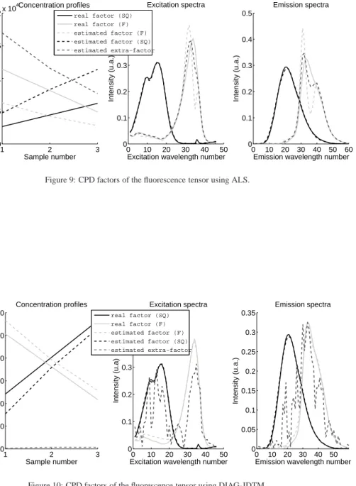
tably the problem of over-factoring is addressed. Finally a concrete application to fluorescence 58
spectroscopy is proposed in section 5. 59
2. Joint eigenvalue decomposition of non-defective matrices
60
We use the following consistent notations in the whole paper: vectors, matrices and tensors 61
are denoted by lower case boldface (a), upper case boldface ( A) and upper case boldface calli-62
graphic (A) letters respectively. The i-th entry of vector a is denoted by aiwhile Ai jis the (i,
j)-63
th component of matrix A. Entry (i1, . . . ,iQ) of any Q-order tensorT ∈ R
I1×···×IQ or
C
I1×···×IQ
64
(Q >2) is denoted byTi1,···,iQ. Outer product, Kronecker product and Khatri-Rao product are
65
denoted by◦,⊗and⊙, respectively. Moore-Penrose matrix inverse, euclidean and frobenius 66
norm are denoted by♯,kE(k)k
Fandk.kF, respectively. We define [x; y]N=[x; y]∩
N.⌊.⌋denotes
67
the floor function. Complex modulus and conjugate of any complex z are denoted by|z|and z 68
respectively. The imaginary unit is denoted by i. 69
Givens and hyperbolic rotation matrices are denoted by G and H, respectively. For instance in 70
the real case, G(θi j) and H(φi j) are equal to the identity matrix, at the exception of the elements: 71
G(θi j)ii=G(θi j)j j=cos(θi j) G(θi j)i j=−G(θi j)ji=sin(θi j)
H(φi j)ii=H(φi j)j j=cosh(φi j) H(φi j)i j=H(φi j)ji=sinh(φi j)
The JEVD problem consists in finding an eigenvector matrix A from a set of non-defective 72
matrices M(k)satisfying: 73
∀k∈[1; K]N, M
(k)=A D(k)A−1, (1) where the K diagonal matrices D(k)are unknown. One could solve these EVDs separately, and 74
retain the solution that leads to the best estimate regarding the considered application. However, 75
as explained in [29], it is safer from a numerical point of view to decompose the K matrices 76
M(k)simultaneously, in some optimal sense, especially when the perturbation of these matrices 77
may have caused eigenvalues to cross each other. Indeed, in practice only noisy observations 78
of the K matrices M(k)are clustered and it is well known that, when eigenvalues are close, the 79
eigenvectors in a single EVD may be strongly affected by small perturbations [33]. The reason is 80
that for coinciding eigenvalues only the corresponding eigenspace is defined; different directions 81
in this subspace will emerge as eigenvectors for different infinitesimal perturbations. When this 82
happens for one or more of the matrices in the JEVD problem, the other matrices may still allow 83
to identify the actual eigenvectors. This follows theorem proved in [29]: 84
Theorem 1. The JEVD is unique up to a permutation and a scaling of the columns of A if and
85
only if all the columns of the K ×N matrix E, whose (k,n)-th component Ek,nis equal to D(k)n,n, 86
are not proportional.
87
Note that in order to ensure uniqueness of the JEVD up to permutation and scale indeterminacies, 88
we will assume in the sequel that the K involved diagonal matrices D(k)fulfil the condition given 89
in Theorem 1. 90
Few papers have proposed numerical solutions to the JEVD problem. All of them adapted 91
Jacobi’s principle to the search for a non-singular and non-necessarily orthogonal eigenmatrix A 92
by using a suitable factorization, which is not reduced to the product of Givens matrices. This 93
domination of Jacobi-like methods is due to their good convergence properties [34]. 94
Two main kinds of Jacobi-like algorithms have been developed in this context, based on dif-95
ferent matrix factorizations. Originally, several authors had recourse to the QR factorization of A 96
in order to compute the different sets of eigenvalues [35, 36]. Arguing that these QR-algorithms 97
suffer from convergence problems, Fu and Gao proposed an effective sh-rt algorithm [37] based 98
on the polar decomposition. Indeed the polar decomposition has been used favourably for eigen-99
value decomposition purpose since a long time [38, 39, 34] and also for joint diagonalization 100
by congruence [40]. Then the JUST algorithm was introduced in [41] as a variation of the sh-rt 101
approach for which the iterative computation of the hyperbolic matrix is made by minimizing an 102
alternative criterion. We propose here a third criterion and an appropriate optimization method, 103
giving birth to the JDTM algorithm. Another JEVD approach based on LU factorization and 104
called JET was introduced in [32] for real-valued matrices. 105
The real case is addressed in the three following subsections. The extension to the complex case 106
is described in subsection 2.4. JDTM algorithm has been compared to JUST and sh-rt algorithms 107
in various situations involving real matrices. Significant numerical results are given in section 108 4.1. 109 110 2.1. A Jacobi-like process 111
In this subsection, all matrices are square matrices of order N. Polar matrix decomposition 112
states that any non-singular real matrix can be factorized into the product of an orthogonal matrix 113
Q and a symmetric positive semidefinite matrix S. It is well known that Q can be decomposed
114
into a product of Givens rotation matrices G(θi j) and a unitary diagonal matrix. In the same way, 115
it has been shown that S can be decomposed into a product of hyperbolic rotation matrices H(φi j) 116
and diagonal matrices [40]. Thereby, due to the indeterminacies of the JEVD problem mentioned 117
in theorem 1 and taking into account that diagonal, hyperbolic and Givens matrices commute, 118
the matrix A solving the JEVD problem given by (1) can be chosen as a product of Givens and 119
hyperbolic rotation matrices: 120 A= N−1 Y i=1 N Y j=i+1 G(θi j)H(φi j). (2)
Inserting (2) into (1) and using the fact that H(φi j)−1=H(−φi j) we get: 121 ∀k∈[1; K]N, D (k)= N−1 Y i=1 N Y j=i+1 G(θi j)TH(−φi j) M(k) N−1 Y i=1 N Y j=i+1 G(θi j)H(φi j) , (3)
but we prefer the simpler formulation: 122 ∀k∈[1; K]N, D (k)= M Y m=1 H(−φm)G(θm)T M(k) M Y m=1 G(θm)H(φm) , (4)
where each integer m of [1; M]Nstands for a couple (i,j) with 1≤i< j≤N. It is worth
men-123
tioning that any Givens or hyperbolic matrix is defined by only one parameter (angle). Therefore, 124
ideally we have to find a set of M=N(N−1)/2 couples of parameters{(θi j, φi j)}1≤i<j≤N in order 125
to get (1). Instead of simultaneously identifying these M couples of parameters, a Jacobi-like 126
procedure will repeat sequences of 2M successive optimizations until convergence. Each opti-127
mization is performed with respect to only one parameter. A sequence of 2M optimizations is 128
generally called a sweep. As a result, NsM couples of Givens and hyperbolic matrices are used
129
in practice to identify A, where Nsis the number of sweeps. We thus look for a matrix A of the 130 form A=QNs ns=1 QM m=1G(θ ns m)H(φ ns
m). The idea is to iteratively diagonalize the M(k)matrices by 131
sequentially optimizing with respect toθns
m andφ ns
m for each value of m and ns. Hence the first 132
sweep (ns=1) consists on the following transformations: 133 ∀k∈[1; K]N, N (k,1,1) = G(θ1 1) TM(k)G(θ1 1), (5) ∀(k,m)∈[1; K]N×[1; M]N, M (k,m,1) = H(−φ1 m)N (k,m,1)H(φ1 m). (6) ∀(k,m)∈[1; K]N×[2; M]NN (k,m,1) = G(θ1 m)TM(k, m−1,1)G(θ1 m) (7) Then the following sweeps (1<ns≤Ns) follow the same scheme:
134 ∀(k,ns)∈[1; K]N×[2; Ns]N, N (k,1,ns) = G(θns 1 ) TM(k,M,ns−1)G(θns 1), (8) ∀(k,m,ns)∈[1; K]N× ∈[1; M]N×[2; Ns]N, M (k,m,ns) = H(−φns m)N(k,m,ns)H(φnms). (9) ∀(k,m,ns)∈[1; K]N× ∈[2; M]N×[2; Ns]N, N (k,m,ns) = G(θns m) TM(k,m−1,ns)G(θns m), (10) Thereby, the optimal corresponding Givens and hyperbolic matrices are sequentially com-135
puted in order to get K diagonal matrices M(k,M,Ns)at the end of the process.
136
2.2. Optimization of matrix angles
137
A natural criterion to compute the optimal (m,ns)-th Givens angleθns
m is thus to minimize the 138
sum of the euclidean norms of the off-diagonal terms of the K matrices N(k,m,ns):
139 ζG(θmns)= K X k=1 N,N X p=1,q=1 p,q N(k,m,ns) pq 2 . (11)
This criterion is the generalization of the original Jacobi criterion to the joint diagonalization 140
context. Since Givens matrices are orthogonal, the same definition of N(k,m,ns)holds in both the
141
joint diagonalization by congruence and JEVD cases and thus the same optimization algorithms 142
can be used. For instance, our proposed algorithm resorts to the same approach as the JAD 143
algorithm described in [42] whereas the sh-rt and JUST algorithms use their own minimization 144
scheme. 145
Once the optimal Givens matrix G(θns
m) is computed, different criteria can be used for the 146
optimal computation of H(φns
m). This is the main difference between the three JEVD algorithms. 147
The sh-rt method aims at minimizing the Frobenius norm of M(h,m,ns) where h is found such
148 thatM(h,m,ns) ii −M (h,m,ns) j j = max 1≤k≤K M(k,m,ns) ii −M (k,m,ns) j j
, whereas the JUST algorithm resorts to 149
criterion (11) by replacing N(k,m,ns) by M(k,m,ns). Instead of minimizing all the (off-diagonal)
150
entries, we propose to target two particular off-diagonal entries of M(k,m,ns): if m corresponds to
151
the (i,j)i<jcouple, we simply aim at computing the optimal M (k,m,ns)
i j and M
(k,m,ns)
ji components by 152
using a "targeting" hyperbolic matrix. It is noteworthy that the transformation (9) affects the i-th 153
and j-th rows and the i-th and j-th columns of Mk,m,nsbut only the (i,j) and the ( j,i) components
154
are twice affected by the hyperbolic matrix and its inverse. Hence our choice to focus on the latter. 155
Therefore, our Joint Diagonalization algorithm based on Targeting hyperbolic Matrices (JDTM) 156
resorts to the following alternative criterionζJDT M
H for the computation of the hyperbolic matrix: 157 ζJDT M H (φ ns m)= K X k=1 M(k,m,ns) i j 2 +M(k,m,ns) ji 2 , (12)
Targeting some components was originally proposed by Souloumiac in a different context [40]. 158
In the case of Givens matrices we showed that the optimizations of criteria (11) and (12) were 159
mathematically equivalent. 160
Now, let us look at the components of M(k,m,ns). As previously mentioned, we only consider the
161
(i,j)-th and ( j,i)-th components which are given by:
162 M(k,m,ns) i j = N(k,m,ns) ii −N (k,m,ns) j j sinh(2φnm)s 2 +N (k,m,ns) i j cosh(φ ns m)2−N (k,m,ns) ji sinh(φ ns m)2, (13) 163 M(k,m,ns) ji = N(k,m,ns) j j −N (k,m,ns) ii sinh(2φns m) 2 −N (k,m,ns) i j sinh(φ ns m) 2+N(k,m,ns) ji cosh(φ ns m) 2. (14) Furthermore we can write that:
164 M(k,m,ns) i j 2 +M(k,m,ns) ji 2 = M(k,m,ns) i j +M (k,m,ns) ji 2 2 + M(k,m,ns) i j −M (k,m,ns) ji 2 2 . (15)
The first term of the right-hand side does not depend onφns
m. Indeed, we derive from (13) and 165
(14) the following equality: 166 M(k,m,ns) i j +M (k,m,ns) ji 2 2 = N(k,m,ns) i j +N (k,m,ns) ji 2 2 . (16) Thereby minimizingζJT DM
H is equivalent to minimize theλfunction defined by: 167 λ(φns m)= K X k=1 M(k,m,ns) i j −M (k,m,ns) ji 2 . (17)
We denote by y(m,ns) the column vector of
R K defined by y(m,ns) k = M (k,m,ns) i j −M (k,m,ns) ji , so that 168 λ(φns
m)=y(m,ns)Ty(m,ns). It is easily shown that the system of linear equations (13) and (14) can be 169
rewritten such that: 170 y(m,ns) =W(m,ns)x(φns m), (18) with: 171 W(m,ns)= N(1,m,ns) ii −N (1,m,ns) j j N (1,m,ns) i j −N (1,m,ns) ji .. . ... N(K,m,ns) ii −N (K,m,ns) j j N (K,m,ns) i j −N (K,m,ns) ji ; x(φ ns m)= " sinh(2φns m) cosh(2φns m) # .
Now defining the diagonal 2 ×2 matrix J such that J11 = −J22 = −1 and observing that 172
x(φns
m)TJ x(φ ns
m) = 1, we have thus to minimize the quantity x(φ ns
m)TW(m,ns)TW(m,ns)x(φ ns
m) under 173
the constraint that x(φns
m)TJ x(φ ns
m)=1. This can be done using the Lagrange multipliers strategy. 174
Thereby, we have to minimize the L function given by: 175
L(x(φns
m), µ(φnms))=x(φmns)TW(m,ns)TW(m,ns)x(φnms)−µ(φnms)x(φnms)TJ x(φnms). (19) Differentiation with respect to x(φns
m) leads to: 176 W(m,ns)TW(m,ns)x(φns m)=µ(φ ns m)J x(φ ns m). (20) Since J−1=J we have: 177 JW(m,ns)TW(m,ns)x(φns m)=µ(φ ns m)x(φ ns m). (21) Thus, µ(φns m) and x(φ ns
m) are associated eigenvalue and eigenvector of matrix JW(m,ns)TW(m,ns). 178
More particularly, we have the following lemma: 179
Lemma 1. If the columns of W(m,ns)are different then JW(m,ns)TW(m,ns) has two nonzero
eigen-180
values of opposite sign and x(φns
m) is the eigenvector associated to the positive eigenvalue. 181
Proof 1. Let w1and w2 be the column vectors of matrix W(m,ns). Both belong toR
K, equipped 182
with the Euclidean norm and we define a=w1Tw1, b=w1Tw2and c=w2Tw2. Hence a, b and c 183
denote the squared euclidean norm of w1, the scalar product between w1and w2and the squared 184
Euclidean norm of w2respectively. Hence, 185 JW(m,ns)TW(m,ns) = " −a −b b c #
The characteristic polynomial is then:
186
P(α)=α2+(a−c)α+(b2−ca) (22)
and the discriminant is:
187
∆ = (a−c)2−4b2+4ca
= (a+c−2b)(a+c+2b)
= ||w1−w2||2||w1+w2||2
Thereby, since w1 ,w2,∆>0 and JW(m,ns)TW(m,ns) is diagonalizable and admits two distinct 188
eigenvaluesα1andα2. Then we have: 189 α1α2 = (a−c)2−∆ 4a2 = b 2−ac a2
The Cauchy-Schwartz inequality gives b2<ac henceα 1α2<0. 190
We now demonstrate the second part of the lemma. Multiplying (21) by x(φns
m)TJ yields: 191 x(φns m) T W(m,ns)T W(m,ns)x(φns m) = µ(φ ns m)x(φ ns m) T J x(φns m), = µ(φns m). (23)
The quadratic form x(φns
m)TW(m,ns)TW(m,ns)x(φ ns m) is positive thusµ(φ ns m) is positive too. 192 7
Hence the previous lemma allows us to easily compute x(φns
m) from W(m,ns) andφ ns
m is deduced 193
from the definition of x(φns
m): 194 φns m = 1 2atanh x(φns m)1 x(φns m)2 ! . (24)
Algorithm 1 summarizes the proposed method.
Algorithm 1: Summary of the JDTM algorithm 1: Define athresholdεand a maximal number of sweep Nmaxs 2: Initialize A with the identity matrix;
3: ns=1; 4: whilePk P p,q(M (k) p,q)2> εand ns≤Nsmaxdo 5: m=1; 6: for i=1 to N−1 do 7: for j=i+1 to N do
8: Compute the optimal angleθns
m corresponding to the couple (i,j) and build G(θ ns
m); 9: Replace the K matrices M(k)by G(θns
m)TM(k)G(θ ns
m); 10: Compute the optimal angleφns
m corresponding to the couple (i,j) and build H(φ ns
m); 11: Replace the K matrices M(k)by H(−φns
m)M(k)H(φ ns m); 12: Replace A by AG(θns m)H(φ ns m); 13: m=m+1; 14: end for 15: end for 16: ns=ns+1; 17: end while 18: Ns=ns; 195 2.3. Computational complexity 196
The computational complexity of an algorithm is given by the numberΓof floating point 197
operations (flop), given in practice by the number of required multiplications. At each sweep, 198
there are N(N−1)/2 Givens and hyperbolic matrices to compute and as many updates of ma-199
trices A,M(1),· · ·,M(K). Computation of each hyperbolic matrix is dominated by the product 200
JW(m,ns)TW(m,ns)which requires 3K multiplications. Givens matrices are computed in a similar
201
way [42] and thus also need 3K multiplications. For each update (line 12 of algorithm 1), matrix 202
A is multiplied by a Givens and a hyperbolic matrix. Both products can be done using a total of
203
8N multiplications. Finaly the update of each matrix M(k)(lines 9 and 11 of algorithm 1) is twice 204
more costly and involves 16N multiplications. Therefore the total computational complexity is: 205
ΓJDT M =NsN(N−1)(3K+4N+8KN) (25)
2.4. Extension to the complex case
206
Let’s now consider that matrices A and M(1),· · ·,M(K)belong to the complex field. In this 207
case, the JDTM algorithm has to be significantly modified. Indeed, each of the Givens and 208
hyperbolic rotation matrices involved in the polar decomposition of a complex matrix is now 209
defined by two parameters. Similarly to the real case, we only focus on the determination of 210
hyperbolic matrices H which makes the specificity of the proposed algorithm. Indeed, G can 211
still be estimated by the classic procedure [42]. 212
We resort to the following classical parametrization of complex hyperbolic matrices, for each 213
couple m=(i,j)i<jwe have: 214
H(φm, αm)ii=H(φm, αm)j j=cosh(φm); H(φm, αm)i j=H(φm, αm)ji=sinh(φm)eiαm
Thereby we have to estimate for each matrix the couple (φi j, αi j) that minimizes the new 215 JDTM cost function: 216 ζJDT M HC (φ ns m, α ns m)= K X k=1 |M(k,m,ns) i j | 2+|M(k,m,ns) ji | 2. (26)
Using the previous parametrization, we obtain: 217 M(k,m,ns) i j = N(k,m,ns) ii −N (k,m,ns) j j sinh(2φns m) 2 e −iαns m +N(k,m,ns) i j cosh(φ ns m) 2− N(k,m,ns) ji sinh(φ ns m) 2 e−2iαnsm, (27) 218 M(k,m,ns) ji = N(k,m,ns) j j −N (k,m,ns) ii sinh(2φns m) 2 e iαns m −N(k,m,ns) i j sinh(φ ns m) 2e2iαns m +N(k,m,ns) ji cosh(φ ns m) 2. (28) It can be easily shown that minimizingζJDT M
HC is equivalent to minimizing ˜ζ JDT M HC : 219 ˜ ζJDT M HC (φ ns m, α ns m)= K X k=1 |M˜(k,m,ns) i j +M (k,m,ns) ji | 2+|M˜(k,m,ns) i j −M (k,m,ns) ji | 2, (29) where: 220 ˜ M(k,m,ns) i j = N(k,m,ns) ii −N (k,m,ns) j j sinh(2φns m) 2 e iαns m +N(k,m,ns) i j cosh(φ ns m) 2e2iαns m −N(k,m,ns) ji sinh(φ ns m) 2. (30) After some straightforward computations, (28), (29) and (30) yield:
221 ˜ ζJDT M HC (φ ns m, αnms)= K X k=1 N(k,m,ns) i j 2+N(k,m,ns) ji 2cosh(2φns m)2 +N(k,m,ns) ii −N (k,m,ns) j j 2−N(k,m,ns) i j N (k,m,ns) ji e2iα ns m +N(k,m,ns) i j N (k,m,ns) i j e−2iα ns m sinh(2φns m)2 +1 2 N(k,m,ns) ii −N (k,m,ns) j j N(k,m,ns) i j − N(k,m,ns) ii −N (k,m,ns) j j N(kji,m,ns) eiαnsm sinh(4φns m) +12N(k,m,ns) ii −N (k,m,ns) j j N(ki j,m,ns)−N (k,m,ns) ji N(k,m,ns) ii −N (k,m,ns) j j e−iαnsm sinh(4φnms) (31) 222
which can be rewritten as a function of 4φns
mandα ns m: 223 ˜ ζJDT M HC (4φ ns m, αnms)= 12 K X k=1 N(k,m,ns) i j 2+N(k,m,ns) ji 2 cosh(4φns m)+1 +N(k,m,ns) ii −N (k,m,ns) j j 2−N(k,m,ns) i j N (k,m,ns) ji e2iα ns m +N(k,m,ns) i j N (k,m,ns) i j e−2iα ns m cosh(4φns m)−1 +N(k,m,ns) ii −N (k,m,ns) j j N(k,m,ns) i j − N(k,m,ns) ii −N (k,m,ns) j j N(kji,m,ns) eiαnsm sinh(4φns m) +N(k,m,ns) ii −N (k,m,ns) j j N(ki j,m,ns)−N (k,m,ns) ji N(k,m,ns) ii −N (k,m,ns) j j e−iαnsm sinh(4φnms). (32) 9
224
Differentiating (32) with respect to 4φns
m andα ns
m alternatively, then defining t ns m =tanh(2φ ns m) and zns m =eiα ns
m, it can be shown after few more trivial computations that the solution couple which
minimizes ˜ζJDT M
HC is also a solution of the following polynomial system:
P0(znms)+(2P1(znms)tnms+P0(znms)tmns)tnms =0 (33) Q1(znms)t ns m −Q0(znms) tns m =0 (34) with: 225 P0(z)= K X k=1 N(k,m,ns) ii −N (k,m,ns) j j N(k,m,ns) i j − N(k,m,ns) ii −N (k,m,ns) j j N(kji,m,ns) z3 +N(k,m,ns) ii −N (k,m,ns) j j N(ki j,m,ns)−N (k,m,ns) ji N(k,m,ns) ii −N (k,m,ns) j j z P1(z)= K X k=1 −N(kji,m,ns)N (k,m,ns) i j z 4+ N(k,m,ns) i j 2+N(k,m,ns) ji 2+N(k,m,ns) ii −N (k,m,ns) j j 2z2−N(ki j,m,ns)N (k,m,ns) ji Q0(z)= K X k=1 N(k,m,ns) ii −N (k,m,ns) j j N(k,m,ns) i j − N(k,m,ns) ii −N (k,m,ns) j j N(kji,m,ns) z3 −N(k,m,ns) ii −N (k,m,ns) j j N(ki j,m,ns)−N (k,m,ns) ji N(k,m,ns) ii −N (k,m,ns) j j z Q1(z)= K X k=1 2 N(kji,m,ns)N (k,m,ns) i j z 4− N(ki j,m,ns)N (k,m,ns) ji (35)
Solution sets are then easily given by: 226 P0(znms)=0 and t ns m =0; (36) or: 227 P0(znms)(Q1(znms)) 2+2P 1(znms)Q0(znms)Q1(zmns)+P0(zmns)(Q0(znms)) 2=0 and tns m = Q0(znms) Q1(znms) . (37)
3. Toward a new direct CPD algorithm: the DIAG method
228
3.1. The Canonical Polyadic Decomposition
229
CPD states that any Q-order tensor (or Q-way array)T of size I1× · · · ×IQcan be exactly 230
decomposed into a sum of Q-order rank-1 tensors. A Q-order rank-1 tensor can be defined as the 231
outer product between Q vectors x(1),· · ·,x(Q). The rank R ofT is then the minimal number of 232
rank-1 tensors needed to achieve the following decomposition: 233 T = R X r=1 x(1)r ◦ · · · ◦x(Q)r . (38)
Usually one also defines Q "loading" (or factor) matrices X(1),· · ·,X(Q)of size I
1×R,· · ·, 234
IQ×R, respectively, so that x (q)
r is the rthcolumn of X(q)and the CPD is commonly rewritten as: 235 ∀q∈[1; Q]N, ∀iq∈[1; Iq]N, Ti1···iQ = R X r=1 Xi(1) 1rX (2) i2r· · ·X (Q) iQr. (39)
Our main problem is thus to find for a given tensorT of given rank R and order Q, the Q factor 236
matrices that solves (39). 237
3.2. Unfolding matrix
238
It is well known that the CPD can be rewritten in a matrix form. Indeed, the tensor dimensions 239
can be merged in order to store all tensor entries in a single "unfolding" matrix. Obviously, there 240
are many way to merge the tensor dimensions and thus many possible unfolding matrices. As it 241
will be seen, the choice of the unfolding matrix has an impact on the algorithm limitations and 242
performance. Therefore, in order to cover all the possibilities, we introduce a P parameter in 243
order that the P first dimensions are merged into the matrix rows whereas the remaining Q−P
244
dimensions are merged into the matrix columns. The corresponding unfolding matrix is denoted 245
by T(P). Note that all the other unfolding matrices can be merely obtained by permuting the 246
tensor dimensions and changing the P value. T(P) entries are linked toT entries by the following 247 transfer formulas: 248 ∀(m,n)∈[1;πP 1]N×[1;π Q P+1]N, T(P)m,n=Ti1,···,iQ (40) where,πa a=Ia,πba=IaIa+1· · ·Iband: 249 ∀m∈[1;πP 1]N, m =i1+ P X q=2 (iq−1)πq−1 1, (41) ∀n∈[1;πQP+1]N, n =iP+1+ Q X q=P+2 (iq−1)π q−1 P+1. (42)
Then after some computations the CPD equation (39) can be rewritten as: 250
T(P)=X(P)⊙ · · · ⊙X(1) X(Q)⊙ · · · ⊙X(P+1)T. (43) It is worth mentioning that a majority of CPD algorithms such as ALS or CFS resorts to the 251
P=1 case. 252
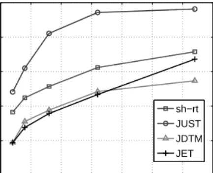
3.3. The DIAG algorithm
253
The algorithm presented here is available both in the real and complex field. We start from 254
equation (43) and we define for a given couple of integers a and b, a<b, the matrix Y(bX,a)by: 255
Y(bX,a)=X(b)⊙ · · · ⊙X(a). (44) Now, let USVHbe the singular value decomposition of T(P) truncated at the order R, assuming 256
that R≤min(πP 1, π
Q
P+1) (hypothesisH1). Thus there exists an invertible square matrix M of size 257 R×R such that: 258 Y(PX,1) = U M, (45) Y(QX,P+1)T = M−1SVH. (46) 11
Recalling that Y(QX,P+1) = X(Q)⊙Y(Q−1,P+1)
X and using the definition of the Kathri-Rao product, 259
Y(QX,P+1)Tcan be seen as a row block matrix: 260 Y(QX,P+1)T=hφ(1)Y(Q−1,P+1) X T,· · ·,φ(IQ)Y(Q−1,P+1) X Ti, (47)
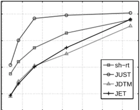
whereφ(1),· · ·,φ(IQ)are the I
Qdiagonal matrices built from the IQrows of the matrix XQ. As a 261
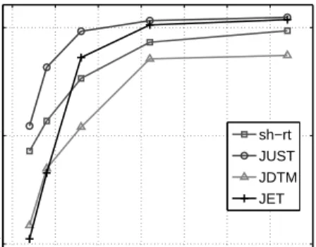
consequence, equations (46) and (47) yield: 262 SVH=hΓ(1)T,· · ·Γ(IQ)T,i, (48) where : 263 ∀i∈[1; IQ]N, Γ(i)=Y(Q−1,P+1) X φ (i) MT. (49) All matricesΓ(i)and Y(QX−1,P+1)are of sizeπQ−P+11×R. We assume that P is chosen so that P<Q−1 264
and R≤πQ−1
P+1 (hypothesisH2) and that they all admit a Moore-Penrose matrix inverse. Then we 265
define: 266
∀i1,i2∈[1; IQ]2N
, i2>i1Θ(i1,i2)=Γ(i1)♯Γ(i2). (50) Now replacingΓ(i)by its definition yields:
267 Θ(i1,i2) = M−T φ(i1)−1Y(Q−1,P+1)♯ X Y (Q−1,P+1) X φ (i2)MT, (51) = M−TΛ(i1,i2)MT, (52)
whereΛ(i1,i2) =φ(i1)−1φ(i2). Thus, M−T performs the JEVD of the known set of matricesΘ(i1,i2). 268
Therefore M−T can be estimated by the JDTM algorithm. Then one can immediately deduce 269
Y(PX,1)and Y(QX,P+1)from (45) and (46). At this stage there are several ways to estimate the factor 270
matrices from Y(PX,1)and Y(QX,P+1). One simple approach is to estimate each column of the first P 271
factor matrices from the corresponding column of Y(PX,1)and each column of the Q−P remaining
272
factor matrices from the corresponding column of Y(QX,P+1). Indeed, column r of Y(PX,1) can be 273
reshaped into an order-P, rank-1 tensorY(PXr,1)whose factor vectors are the r-th columns of matri-274
ces X(1),· · ·,X(P). Thereby a simple rank-1 High-Order SVD (HOSVD, [43]) ofY(P,1)
Xr provides 275
a direct estimation of x(1)r ,· · ·,x (P)
r . In the same way, the column r of Y (Q,P+1)
X can be reshaped 276
in a (Q−P)-order, rank-1 tensorY(Q,P+1)
Xr whose factor vectors are the r-th columns of matrices 277
X(P+1)· · ·X(Q). Hence, x(P+1) r · · ·x
(Q)
r can be estimated from the rank-1 HOSVD ofY (Q,P+1) Xr . Fi-278
nally both operations are repeated for all the r values. The DIAG algorithm is summarized by 279
Algorithm 2. 280
3.4. Computational complexity
281
ΓDIAGis clearly dominated by the three following computations. First, the truncated SVD of 282
the unfolding matrix of size (πP 1, π Q P+1) requires 2π Q P+1(π P 1) 2+5R2(πP 1 +π Q P+1)−2(R 3+(πP 1) 3)/3 283
multiplications, assuming thatπQP+1 > πP
1. Then, the computation of theΘmatrices needs ap-284
proximately (RIQ)2πQ−P+11 additional multiplications. Finally the cost of the JEVD procedure is 285
approximated by 8Ns(IQ)2R3. Additional computations can be neglected and thus we have: 286 ΓDIAG≈2π Q P+1(π P 1) 2+5R2(πP 1+π Q P+1)−2(R 3+(πP 1) 3)/3+(RI Q)2π Q−1 P+1+8Ns(IQ)2R3. (53)
Algorithm 2: Summary of the DIAG algorithm
1: Choose a value of P and a permutation of the dimensions ofT as described in section 3.6;
2: Matricize the (possibly permuted) tensorT into matrix T(P) according to (40), (41) and (42);
3: Compute the SVD USVHof T(P), truncated at rank R;
4: Split SVHinto I
Qblocks of size R×πQP+−11in order to form the IQmatricesΓ(i)given by (49);
5: for i1=1 to IQ−1 do
6: for i2=i1+1 to IQdo
7: ComputeΘ(i1,i2) =Γ(i1)♯Γ(i2);
8: end for 9: end for
10: Compute matrixM−Tby JEVD of the set ofΘ(i1,i2)matrices; 11: Deduce matrices Y(PX,1)=U M and YX(Q,P+1)=M−1SVH;
12: for r=1 to R do
13: BuildY(P,1)
Xr andY (Q,P+1)
Xr by reshaping the r−th columns of Y (P,1) X and Y (Q,P+1) X ; 14: Deduce x(1)r ,· · ·,x (P)
r from the rank 1 HOSVD ofY (P,1) Xr ; 15: Deduce x(Pr +1),· · · ,x
(Q)
r the rank 1 HOSVD ofY (Q,P+1) Xr ;
16: end for
ΓDIAGshould be compared to the numerical complexity of the ALS algorithm which is approxi-287
mately given by: 288 ΓALS ≈NALS 3Rπ Q 1 +7R 2 Q X q=1 Q Y k=1 k,q Ik , (54)
However the numerical complexity of the DIAG algorithm is strongly related to the choice of the 289
unfolding matrix and both complexities depend on a large number of parameters. Furthermore 290
NALScan fluctuate wildly. Therefore at this point it would be very hazardous to draw general con-291
clusions from the previous formulas even in simple cases. Nevertheless we made some extensive 292
flop comparisons between both algorithms by varying Q,R,P and the tensor dimensions. Results
293
are reported in section 4.2.4. It will be shown that in all the considered situationsΓDIAG ≤ΓALS 294
and Ns≪NALS. 295
296
The numerical complexity of the CFS algorithm is very complicated to establish since this 297
algorithm computes several estimations of each factor matrix. However we can easily explain 298
what makes DIAG a cheaper approach. CFS is a three step algorithm. The first step is algebraic 299
and performs the HOSVD of the tensor. In terms of numerical complexity this operation is 300
usually close to the SVD of the unfolding matrix performed in the DIAG algorithm. The second 301
step is the resolution of Q(Q−1)2JEVDs whereas DIAG requires only one JEVD. Finally, we 302
have to choose the best estimates of the factor matrices among a large number of combinations 303
which is also very time consuming. 304
3.5. Necessary conditions to the identifiability of DIAG, ALS and CFS
305
The CPD algorithms are not always applicable due to their intrinsic restricted conditions. 306
We propose to compare here necessary conditions that ensure identifibility of the ALS, CFS and 307
DIAG methods. Let Q, R and I(i) be the tensor order, the CPD rank and the i-th dimension of 308
the tensor, respectively. A tensor of order Q and rank R can be canonically decomposed by ALS 309 only if: 310 (CALS) : ∀q∈[1; Q]N, Q Y i=1 i,q I(i)≥R. (55)
DIAG conditions are given by hypothesesH1andH2.H1andH2 were expounded for a given 311
order of the tensor dimensions (default order). Actually, By taking into account that the dimen-312
sions can be permuted we obtain the following more general condition: 313
(CDIAG) : ∃P∈[2; Q−1]N,∃ fI a permutation of the Q first natural numbers and∃qs>P such that:
QP
i=1I( fI(i))≥R and QQi=P+1 i,qs
I( fI(i))≥R. (56)
Finally, the conditionCCFS for the closed-form solution is given in [28]: 314
(CCFS) :∃(q1,q2)∈[1; Q]2
N
, q1,q2such that I(q1)≥R and I(q2)≥R. (57)
Proposition 1. CDIAGis more restrictive thanCALS but less restrictive thanCCFS:
315
CCFS ⇒ CDIAG⇒ CALS 316
A proof is given in appendix. In practice the DIAG condition implies P ≤ Q−2 and can be 317
reformulated quite easily for low order tensors (3≤Q≤5): 318
Third order tensors, Q=3. Here we have necessarily P=1 henceCDIAGbecomes simply: at
319
least two of the tensor dimensions are greater or equal to the CPD rank R. Thereby at order 320
3 (and only at order 3)CDIAGandCCFS are equivalent. 321
Fourth order tensors, Q=4. Here we can choose either P = 1 or P = 2 but the condition
322
remains the same in both cases and is simply: at least one tensor dimension is greater than 323
R and at least one product of two of the remaining dimensions is also greater than R.
324
Fifth order tensors, Q=5. Here 1≤P≤3:
325
• if we choose P=1 or P=3 thenCDIAGbecomes: at least one tensor dimension is 326
greater than R and at least one product of three of the remaining dimensions is also 327
greater than R. 328
• if we choose P =2 thenCDIAG becomes: at least one product between two tensor 329
dimensions and another product between two of the remaining dimensions are greater 330
than R. 331
3.6. Choice of the unfolding matrix
332
An obvious criterion is the residual error betweenT and the reconstructed tensor built from 333
the estimated factor matrices. However it would be very time consuming to test several possibil-334
ities. As a consequence the choice of the more appropriate unfolding matrix should be related to 335
hypothesisH1 andH2. Indeed, one has to choose a permutation of the tensor dimensions and 336
a P value that ensure both hypotheses. Otherwise, the DIAG algorithm is not suitable as it is 337
explained in the previous section. Recall notably that the DIAG algorithm implies P ≤Q−2. 338
Indeed, at order 3 we have necessarily P = 1. At order 4 we have two possible values (1 and 339
2) and so on. Therefore if one wants to maximize the value of the highest possible rank then 340
one should maximize min(πq−1 1, πq−P+11), hence choose T(p) as squared as possible. In practice 341
we observed that this recommendation is always a good option even if all tensor dimensions are 342
greater than the rank. Apart from that one should note that the number of matrices to be jointly 343
diagonalized is directly related to the squared dimension of the last mode and thus the numerical 344
complexity of the JEVD step. Therefore in the case of a tensor with one very large dimension 345
we do not recommend to put it at the end (if possible). More generally, we recommend to take 346
into consideration the overall complexity of the DIAG algorithm given by equation (53) and to 347
consider that with the JDTM algorithm the number of sweeps (Ns) exceeds very rarely 10. In 348
section 4.2.4 we give several significant numerical examples of DIAG complexity for various 349
tensor dimensions and unfolding matrices. 350
4. Numerical simulations
351
The proposed algorithms are first validated on synthesized data sets. We first focus the JEVD 352
sub-problem for which we compare JDTM performances to these of other JEVD algorithms. 353
Then we compare the DIAG approach with CFS, an other direct algorithm and ALS-ELS which 354
is a reference iterative method, with respect to several scenarios. The last subsection is dedicated 355
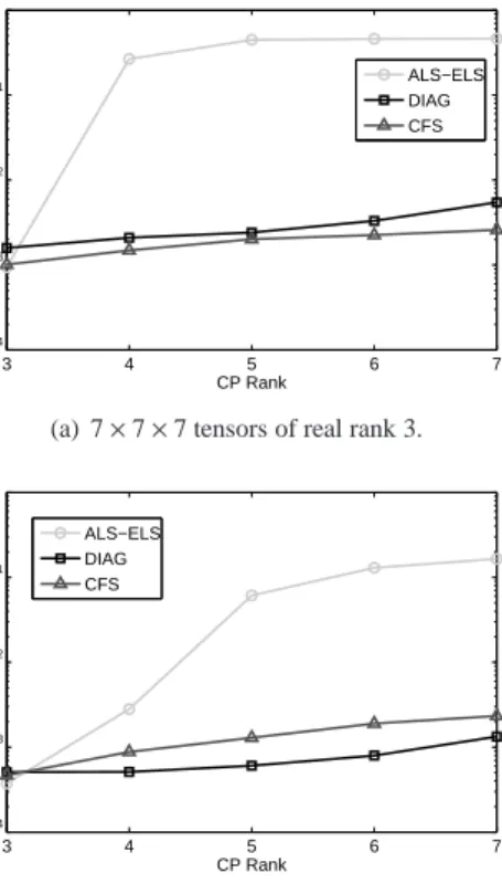
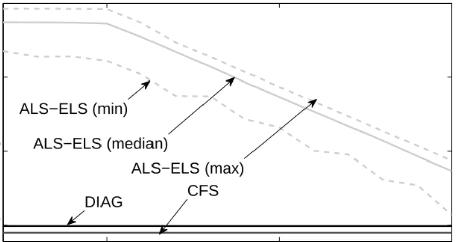
to a particular tensor family for which iterative algorithms consistently fail to find the CPD. 356
4.1. Performance comparison of the JDTM algorithm
357
The performance of the JDTM algorithm is studied and compared to that of the JET, sh-rt 358
and JUST methods by varying the number K of matrices to be jointly diagonalized, the Signal-359
to-Noise Ratio (SNR) and the matrix dimensions N. The matrix set to be jointly diagonalized is 360
built according to the following model: 361 ∀k∈[1; K]N, M (k) = Me (k) kMe(k)kF +σ E (k) kE(k)kF with ˜M(k)= A D(k)A−1. (58) Entries of A, D(k)and E(k)are drawn randomly according to a standard normal distribution. The 362
scalar parameterσallows us to regulate the power of the Gaussian additive noise E(k). The SNR 363
is then equal to−20 log10(σ). Hence,σis chosen in order to obtained the desired value of SNR. 364
At the end of each sweep, the squared off-diagonal components of the K matrices M(k,M,ns)
365
are summed and the obtained value is compared to the value computed at the previous sweep. 366
Algorithms are stopped when the relative deviation between two successive values is smaller 367
than 10−3. 368
After having removed the scaling and permutation indeterminacies we define rAas the rela-369
tive root squared error between the true eigenvector matrix and its estimatebA:
370 rA = v u u u t PN i=1 PN j=1 Ai,j−bAi,j 2 PN i=1 PN j=1 Ai,j 2 . (59)
Note that in most practical applications and notably in blind source separation, one is only inter-371
ested by the estimation of the eigenvector matrix. Hence rAappears as a relevant JEVD criterion. 372
Finally the number of sweeps, Ns, required by each algorithm is stored in order to com-373
pute the values of the total numerical complexitiesΓ. Therefore, algorithm results are judged 374
according to three criteria, namely Ns,Γand rA. 375
Each simulation is repeated 100 times with a new draw of the matrices A, D(k) and E(k) at 376
each time. We present here median values of rAand mean values ofΓand Nsobtained from each 377
algorithm. 378
Figures 1, 2 and 3 show simulation results for 3 SNR values (60 dB, 40 dB and 20 dB 379
respectively). The number of matrices to be jointly diagonalized was fixed to K=64 whereas we 380
varied the matrix size N from 2 to 32. We first note that the estimation precision of the algorithms 381
logically increases with the ratio K/N and the SNR. Second, according to rA criterion JUST 382
algorithm is consistently outperformed by other algorithms whatever the considered situation. 383
At 60 dB, figure 1(a) points out that the JDTM and JET algorithm outclass the sh-rt approach 384
concerning the estimation of eigenvectors matrix. According to this rA criterion JET performs 385
slightly better than JDTM for matrix size lower or equal to 16 whereas for the largest size JDTM 386
clearly provides the best performances. The comparison of the average computational costs 387
displayed in figure 1(b) shows very closed results between all the algorithms. However JDTM 388
appears more clearly as the less costly algorithm for largest matrix sizes. This is explained by a 389
lower and remarkably stable number of sweeps (figure 1(c)). Previous conclusions hold at 40 dB. 390
However it is interesting to note that concerning the estimation of the eigenvectors matrix JDTM 391
is now significantly more accurate than JET for N =16 and N =32. Finally, the 20 dB case 392
highlights the efficiency of the JDTM algorithm which clearly improves JET and sh-rt results, for 393
matrix sizes larger than 8. However JET is now the faster algorithm. In conclusion JDTM appears 394
as a very versatile algorithm which provide very accurate results in all the considered situation 395
(in comparison to its competitors) for a lower number of sweeps. This number is remarkably 396
stable, being comprised between 3 and 10 in all the considered scenarios. Moreover JDTM 397
consistently provides the best estimate of the eigenvector matrix for the largest matrix size and 398
this gap increases with the SNR. To sum up, JDTM offers quite similar performances than its 399
best competitors (sh-rt or JET) in the easiest cases (regarding SNR and K/N ratio) whereas it
400
clearly becomes the better choice as the difficulty increases. 401
As part of this study, we also evaluate JDTM ability to deal with an ill-conditioned eigen-402
vector matrix. For this purpose, we now compute the eigenvector matrix A with pairwise corre-403
lated columns as follows: odd columns, a2r−1, are still randomly drawn as previously but even 404
columns, a2r, are built in the following way : 405
∀r∈[1; N/2]N, a2r=νa2r−1+(1−ν)nr, (60)
where nr is a vector of R
N whose components are randomly drawn according to a standard 406
normal distribution. Therebyνdefines a collinearity factor which will vary from 0.1 to 0.9 so 407
that matrices A can be very ill-conditioned. Figure 4 shows simulation results for a set of 10 408
matrices of size 10 (K=N=10) at 80 dB. It can be seen that sh-rt, JDTM and JET perform well 409
forν <0.9. JDTM and JET provide the best results in terms of estimation precision but JDTM 410
requires a minimal number of sweeps and computational cost. 411
4.2. Performance comparison of the DIAG algorithm
412
We now study performances of the DIAG algorithm for the decomposition of noisy tensors. 413
Indeed, in most practical applications involving tensor analysis, a noisy tensor of rank R is mod-414
0 5 10 15 20 25 30 35 10−10 10−8 10−6 10−4 10−2 100 Matrix size log 10 (ra ) sh−rt JUST JDTM JET
(a) rAcriterion (median)
0 5 10 15 20 25 30
104 106 108
Matrix size
Number of FLOPs (log
10 ) sh−rt JUST JDTM JET (b)Γcriterion (mean) 0 5 10 15 20 25 30 35 0 5 10 15 20 25 30 Matrix size Number of sweeps sh−rt JUST JDTM JET
(c) Number of Sweeps (mean)
Figure 1: Evolution of the three comparison criteria as a function of the matrix size for a set of 64 matrices with an SNR value of 60 dB.
0 5 10 15 20 25 30 10−6 10−4 10−2 100 Matrix size log 10 (ra ) sh−rt JUST JDTM JET
(a) rAcriterion (median)
0 5 10 15 20 25 30 35 102 104 106 108 1010 Matrix size
Number of FLOPs (log
10 ) sh−rt JUST JDTM JET (b)Γcriterion (mean) 0 5 10 15 20 25 30 35 0 5 10 15 20 25 30 Matrix size Number of sweeps sh−rt JUST JDTM JET
(c) Number of Sweeps (mean)
Figure 2: Evolution of the three comparison criteria as a function of the matrix size for a set of 64 matrices with an SNR value of 40 dB.
0 5 10 15 20 25 30 10−4 10−2 100 Matrix size log 10 (ra ) sh−rt JUST JDTM JET
(a) rAcriterion (median)
0 5 10 15 20 25 30 35 102 104 106 108 1010 Matrix size
Number of FLOPs (log
10 ) sh−rt JUST JDTM JET (b)Γcriterion (mean) 0 5 10 15 20 25 30 35 0 5 10 15 20 25 30 Matrix size Number of sweeps sh−rt JUST JDTM JET
(c) Number of Sweeps (mean)
Figure 3: Evolution of the three comparison criteria as a function of the matrix size for a set of 64 matrices with an SNR value of 20 dB.
0 0.2 0.4 0.6 0.8 1 10−4 10−3 10−2 10−1 100 Collinearity factor log 10 (ra ) sh−rt JUST JDTM JET
(a) rAcriterion (median)
0.2 0.4 0.6 0.8
106
Collinearity factor
Number of FLOPs (log
10 ) sh−rt JUST JDTM JET (b)Γcriterion (mean) 0.2 0.4 0.6 0.8 5 10 15 20 25 30 Collinearity factor Number of sweeps sh−rt JUST JDTM JET
(c) Number of Sweeps (mean)
Figure 4: Evolution of the three comparison criteria as a function of the correlated factor between columns of matrix A for a set of 10 matrices of size 10 and an SNR value of 80 dB.
elized by "truncated" CPD of rank Rm<R which is usually more relevant than the exact CPD: 415 ∀q∈[1; Q]N, ∀iq∈[1; Iq]N, Ti 1,···,iQ = Rm X r=1 X(1)i 1,rX (2) i2,r· · ·X (Q) iQ,r+Ei1,···,iQ, (61)
where Eis an error term. Rmis the model rank. The DIAG algorithm is compared with an 416
ALS-ELS algorithm and with the CFS algorithm in various situations by means of Monte-Carlo 417
experiments. For each new experiment, a noise free tensor is built from factor matrices of Rm 418
columns whose entries are randomly drawn according to a standard normal distribution. We then 419
add a Gaussian white noise whose the power is regulated according to the desired SNR value. 420
The comparison criterion, rX, is the Normalized Mean Squares Error (NMSE) computed between 421
actual and estimated factor matrices. Hence for a tensor of order Q we have: 422 rX = 1 Q Q X q=1 med v t vec(X(q)−Xd(q))Tvec(X(q)−Xd(q)) vec(X(q))Tvec(X(q)) , (62)
where Xd(q) denotes the estimation of the factor matrix X(q), the vec(·) operator maps a matrix 423
to a column vector by stacking its columns one below the other and med(·) denotes the median 424
value computed from 100 MC experiments. Permutation and scaling ambiguities in the estimated 425
factor matrices are fixed in the same manner as in [21]. All algorithms were written in-house. The 426
ALS-ELS algorithm can be found in the tensor package web-page1. It is stopped as soon as the 427
relative deviation between two consecutive values of the CPD cost function becomes lower than 428
10−6or the number of ALS iterations reaches 1000. ELS procedure is run every 5 iterations. For 429
the decomposition of order-3 tensors, we use the CFS algorithm described in [27] with the best 430
matching scheme proposed in section 4.2 of [27] whereas higher order tensors were decomposed 431
using the N-order version described in [28], using the sub-optimal matching rules proposed by 432
the authors. Implemented versions of DIAG and CFS resort to the JDTM algorithm to solve the 433
JEVD problem and are stopped as soon as the relative deviation between two consecutive values 434
of the JEVD cost function becomes lower than 10−6 or the number of JEVD iterations reaches 435
30. Unfolding matrix in the DIAG algorithm is generally chosen to be as squared as possible. 436
Since the number of test parameters is large, it would be impossible to perform here an exhaustive 437
comparison. As a consequence we have limited ourselves to some key situations which illustrate 438
the main features of the proposed approach : i. its ability to decompose high order tensors of 439
high rank, ii. tensors with almost collinear factors, iii. its insensitivity to over-factoring and iv. 440
its low computational complexity. 441
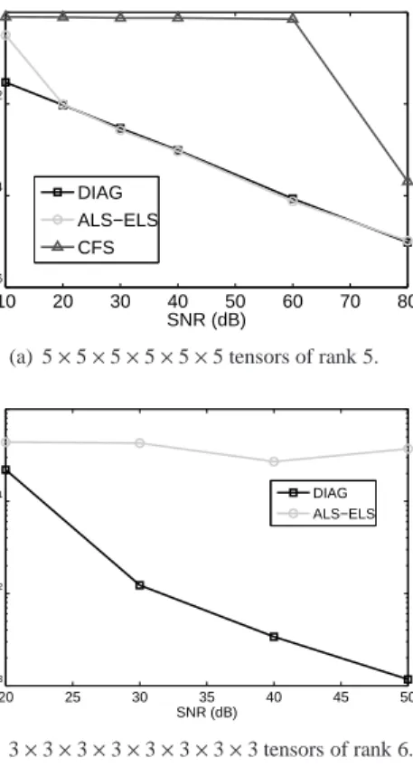
4.2.1. High order tensors
442
We first consider a set of 6-order tensors of rank 5 whose all the dimensions are equal to 5. 443
DIAG parameter P is set to 3 and we vary the SNR from 10 dB to 80 dB. Results are plotted 444
on figures 5(a). CFS only works for the highest SNR value, probably because this is a difficult 445
situation for which we are very close to its intrinsic limitation. DIAG provides as accurate 446
estimations as ALS-ELS for SNR values greater than 10 dB. ALS-ELS fails at 10 dB while 447
DIAG still works. Notably it clearly outperforms ALS at 10 dB. 448
1http://www.gipsa-lab.grenoble-inp.fr/~pierre.comon/TensorPackage/tensorPackage.html
10 20 30 40 50 60 70 80 10−6 10−4 10−2 100 SNR (dB) NMSE DIAG ALS−ELS CFS
(a) 5×5×5×5×5×5 tensors of rank 5.
20 25 30 35 40 45 50 10−3 10−2 10−1 100 SNR (dB) NMSE DIAG ALS−ELS (b) 3×3×3×3×3×3×3×3 tensors of rank 6.
Figure 5: Median NMSE as a function of the SNR at the output of the ALS and DIAG algorithms applied to high order tensors.