Identifying disease-associated genes based on artificial intelligence

(1)

Identifying disease-associated genes based on artificial intelligence

A Thesis Submitted to the

College of Graduate and Postdoctoral Studies

in Partial Fulfillment of the Requirements

for the degree of Doctor of Philosophy

in the Division of Biomedical Engineering

University of Saskatchewan

Saskatoon

By

Ping Luo

c

(2)

Permission to Use

In presenting this thesis in partial fulfilment of the requirements for a Postgraduate degree from the University of Saskatchewan, I agree that the Libraries of this University may make it freely available for inspection. I further agree that permission for copying of this thesis in any manner, in whole or in part, for scholarly purposes may be granted by the professor or professors who supervised my thesis work or, in their absence, by the Head of the Department or the Dean of the College in which my thesis work was done. It is understood that any copying or publication or use of this thesis or parts thereof for financial gain shall not be allowed without my written permission. It is also understood that due recognition shall be given to me and to the University of Saskatchewan in any scholarly use which may be made of any material in my thesis. Requests for permission to copy or to make other use of material in this thesis in whole or part should be addressed to:

Head of the Devision of Biomedical Engineering Engineering Building

57 Campus Drive

University of Saskatchewan Saskatoon, Saskatchewan S7N 5A9 Canada

OR

Dean of College of Graduate and Postdoctoral Studies Room 116 Thorvaldson Building

110 Science Place

University of Saskatchewan Saskatoon, Saskatchewan S7N 5C9 Canada

(3)

Abstract

Identifying disease-gene associations can help improve the understanding of disease mechanisms, which has a variety of applications, such as early diagnosis and drug development. Although experimental tech-niques, such as linkage analysis, genome-wide association studies (GWAS), have identified a large number of associations, identifying disease genes is still challenging since experimental methods are usually time-consuming and expensive. To solve these issues, computational methods are proposed to predict disease-gene associations.

Based on the characteristics of existing computational algorithms in the literature, we can roughly divide them into three categories: network-based methods, machine learning-based methods, and other methods. No matter what models are used to predict disease genes, the proper integration of multi-level biological data is the key to improving prediction accuracy. This thesis addresses some limitations of the existing computational algorithms, and integrates multi-level data via artificial intelligence techniques. The thesis starts with a comprehensive review of computational methods, databases, and evaluation methods used in predicting disease-gene associations, followed by one network-based method and four machine learning-based methods.

The first chapter introduces the background information, objectives of the studies and structure of the thesis. After that, a comprehensive review is provided in the second chapter to discuss the existing algorithms as well as the databases and evaluation methods used in existing studies. Having the objectives and future directions, the thesis then presents five computational methods for predicting disease-gene associations.

The first method proposed in Chapter 3 considers the issue of non-disease gene selection. A shortest path-based strategy is used to select reliable non-disease genes from a disease gene network and a differential network. The selected genes are then used by a network-energy model to improve its performance. The second method proposed in Chapter 4 constructs sample-based networks for case samples and uses them to predict disease genes. This strategy improves the quality of protein-protein interaction (PPI) networks, which further improves the prediction accuracy. Chapter 5 presents a generic model which applies multimodal deep belief nets (DBN) to fuse different types of data. Network embeddings extracted from PPI networks and gene ontology (GO) data are fused with the multimodal DBN to obtain cross-modality representations. Chapter 6 presents another deep learning model which uses a convolutional neural network (CNN) to integrate gene similarities with other types of data. Finally, the fifth method proposed in Chapter 7 is a nonnegative matrix factorization (NMF)-based method. This method maps diseases and genes onto a lower-dimensional manifold, and the geodesic distance between diseases and genes are used to predict their associations. The method can predict disease genes even if the disease under consideration has no known associated genes.

In summary, this thesis has proposed several artificial intelligence-based computational algorithms to address the typical issues existing in computational algorithms. Experimental results have shown that the proposed methods can improve the accuracy of disease-gene prediction.

(4)

Acknowledgements

I would like to express my sincere gratitude to my supervisor, Prof. Fang-Xiang Wu, who offered me the opportunity to pursue the Ph.D. degree in his lab. Throughout my studies, he constantly provides me insightful suggestions, not only for research but also for my daily life. This work would not have been possible without his help.

I would also like to express my gratitude to other members of my advisory committee, Prof. Ian McQuillan, Prof. Mark Keil, and Prof. Francis Bui. I have received positive support and valuable suggestions from them during the Ph.D. program. Their courses also help me lay a solid foundation for my study.

In addition, I am lucky to learn and work with a group of great colleagues. I am particularly indebted to Yan Yan, Jinhong Shi, Yulian Ding, Pi-Jing Wei, Bolin Chen, Lin Wu, Fei Wang, Lingkai Tang, and Yichao Shen, for their help in both my life and research.

I would also like to thank my friends Wei Chen, Jinglin Gao, Qian Huang, Fan Zhang, Wen-Jing Zhang, Rebecca Mao, Tyler Zhang, Yaogeng Lei, Maodong Zhang, Lizhi Liu, Kang Jiang, and Qi Guo, for sharing their life experience with me, which has broadened my horizons.

Finally, I would like to thank all my families for their unconditional support and love. I am also grateful for the financial support provided by the Natural Sciences and Engineering Research Council of Canada (NSERC), University of Saskatchewan (UofS), the China Scholarship Council (CSC), and the family of Russell Haid.

(5)

This thesis is dedicated to my father Yuedong Luo, my mother Fang Wu, and my grandfather Jiazhang Wu, who encouged me all these years.

(6)

4.2.4 Ensemble prediction . . . 54 4.2.5 Datasets . . . 54 4.2.6 Evaluation metrics . . . 55 4.3 Results . . . 56 4.3.1 Clustering . . . 56 4.3.2 Sensitivity analysis . . . 57 4.3.3 Comparison . . . 58 4.3.4 De novo validation . . . 58 4.4 Discussion . . . 59 4.5 Conclusions . . . 60 4.6 Acknowledgements . . . 60

(8)

5 Enhancing the prediction of disease-gene associations with multimodal deep learning 64

5.1 Introduction . . . 65

5.2 Materials and methods . . . 67

5.2.1 RBM . . . 67

5.2.2 Multimodal DBN . . . 68

5.2.3 Raw feature extraction . . . 68

5.2.4 Evaluation metrics . . . 71

5.2.5 Hyperparameters . . . 72

5.2.6 Data sources . . . 72

5.3 Results . . . 73

5.3.1 Overall performance . . . 73

5.3.2 Comparison with other algorithms . . . 73

5.3.3 Prediction of new disease-gene associations . . . 74

5.4 Conclusion . . . 74

6 deepDriver: predicting cancer driver genes based on somatic mutations using deep convolutional neural networks 79 6.1 Introduction . . . 80

6.2 Material and methods . . . 81

6.2.1 General model . . . 81 6.2.2 Network-based convolution . . . 82 6.2.3 Mutation-based features . . . 82 6.2.4 Data sources . . . 83 6.2.5 Evaluation metrics . . . 84 6.2.6 Implementation . . . 85 6.3 Results . . . 85 6.3.1 Hyperparameters . . . 85 6.3.2 Cross-validation . . . 86 6.3.3 De novo study . . . 86 6.4 Conclusion . . . 87

7 Identifying disease-gene associations with graph-regularized manifold learning 98 7.1 Introduction . . . 99

7.2 Methods and material . . . 100

7.2.1 General model . . . 100

7.2.2 Similarity network . . . 103

(9)

7.2.4 Data sources . . . 104 7.2.5 Evaluation metrics . . . 105 7.3 Results . . . 106 7.3.1 Model parameters . . . 106 7.3.2 Cross-validation . . . 106 7.3.3 De novo study . . . 106 7.4 Conclusion . . . 107 7.5 Acknowledgements . . . 107

8 Summary and future work 110 8.1 Summary . . . 110

8.2 Future work . . . 111

References 112

Appendix A List of Publications 144

(10)

List of Tables

2.1 Some commonly used databases of disease-gene associations . . . 17

2.2 Some commonly used databases of PPI networks . . . 18

2.3 Some commonly used databases of Pathways . . . 20

3.1 Enriched KEGG pathways of candidate genes in the BC dataset . . . 43

3.2 Enriched KEGG pathways of candidate genes in the TC dataset . . . 44

3.3 Enriched KEGG pathways of candidate genes in the AD dataset . . . 46

3.4 Top 10 unknown genes . . . 47

4.1 Sensitivity analysis. The resulted AUC values obtained with different combinations of hyperpa-rameters for BC. . . 58

4.2 Sensitivity analysis. The resulted AUC values obtained with different combinations of hyperpa-rameters for TC. . . 59

4.3 Sensitivity analysis. The resulted AUC values obtained with different combinations of hyperpa-rameters for AD. . . 60

4.4 Top 10 unknown genes . . . 63

5.1 Top-10 associations predicted by dgMDL, Known-GENE and PCFM . . . 77

5.2 Top-10 susceptible lung cancer-associated genes . . . 78

6.1 12 features extracted from mutation data. . . 87

6.2 Top 10 predictions of deepDriver . . . 88

6.3 Top 10 predictions of 20/20+ . . . 89

6.4 Top 10 predictions of SVM . . . 90

6.5 Top 10 predictions of OncodriveCLUST . . . 91

(11)

List of Figures

2.1 Classification of existing computational methods for disease gene prediction. . . 6

2.2 Schematic example of a random walk. The network contains 50 nodes (genes), in which 15 of them are disease-associated. Their corresponding entries inP0are equal to 1. The random walk is performed with a restart probability ofr= 0.5, and it reaches a stead state whent= 17. . . . 8

2.3 Classic pipeline of supervised machine learning-based methods. . . 12

2.4 Eight types of evidence valuable for disease gene prediction. The five types of evidence in the left blue circle characterize the functional similarity of genes, and the two types of evidence in the right yellow circle contain disease-associated information. Gene expression in the middle contain both types of information. . . 16

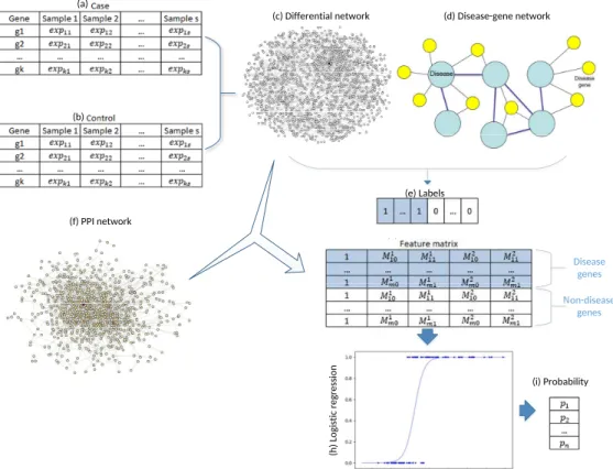
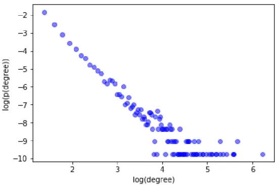
3.1 The work flow of dgSeq. (a)–(b). Clinical RNA-Seq data of the case and control subjects; (c). Differential network constructed by (a) and (b); (d) disease-gene network constructed by OMIM data; (e). Labels of all the genes determined by (c), (d) and benchmark disease genes; (f). PPI network; (g). Feature matrix extracted from (c) and (f); (h). Logistic regression model trained with (e) and (g); (i). The calculated probabilities of all the genes being labeled as 1 (disease gene). 31 3.2 Scatter plot of the log-log degree distribution ofGdif for BC . . . 34

3.3 Sample disease gene network . . . 35

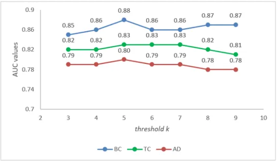
3.4 Sensitivity analysis of thresholdk . . . 39

3.5 The ROC curves of three algorithms in predicting BC-related genes . . . 40

3.6 The ROC curves of three algorithms in predicting TC-related genes . . . 41

3.7 The ROC curves of three algorithms in predicting AD-related genes . . . 42

4.1 Work flow of the algorithm. . . 50

4.2 Hierarchical clustering dendrogram for BC. . . 56

4.3 Hierarchical clustering dendrogram for TC. . . 56

4.4 Hierarchical clustering dendrogram for AD. . . 57

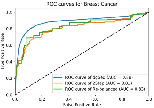
4.5 ROC curves for BC. . . 61

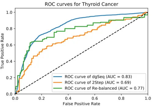
4.6 ROC curves for TC. . . 61

4.7 ROC curves for AD. . . 62

5.1 Schematic example of an RBM. . . 67

5.2 Schematic example of a multimodal DBN for disease gene prediction. . . 75

5.3 AUC of dgMDL in different layers . . . 76

(12)

6.1 Schematic 1-D CNN. In this study, each CONV layer is followed by a pooling layer and the CONV-POOL pattern is repeated for several times. The final structure of the model is determined by

grid search. . . 92

6.2 Construction ofφi. Given the feature vectors ofgi and itsknearest neighborsgs1, gs2, . . . , gsk, a feature matrixφiis constructed by arranging the 2kvectors into a 2k×nf matrix, which is then used in the convolution. . . 93

6.3 ROC curves of the three algorithms obtained on the dataset of BRCA. The red, green and magenta lines depict the ROC curves of deepDriver, 20/20+ and SVM, respectively. The AUC value of deepDriver is 0.984, which is at least 15.1% higher than that of the other two algorithms. 93 6.4 ROC curves of the three algorithms obtained on the dataset of COAD. The red, green and magenta lines depict the ROC curves of deepDriver, 20/20+ and SVM, respectively. The AUC value of deepDriver is 0.976, which is at least 25.5% higher than that of the other two algorithms. 94 6.5 ROC curves of the three algorithms obtained on the dataset of LUAD. The red, green and magenta lines depict the ROC curves of deepDriver, 20/20+ and SVM, respectively. The AUC value of deepDriver is 0.998, which is at least 24.9% higher than that of the other two algorithms. 95 6.6 Learning curve for BRCA. . . 95

6.7 Learning curve for COAD. . . 96

6.8 Learning curve for LUAD. . . 96

6.9 ROC curves of deepDriver obtained from the second sets of driver genes. . . 97

7.1 ROC curves of the three competing algorithms on multiple-gene diseases. . . 108

(13)

List of Abbreviations

AD Alzheimer’s Disease AI Artificial Intelligence AUC Area Under the ROC Curve

AUPR Area Under the Precision-Recall Curve BBRBM Binary-Binary RBM

BC Breast Cancer

BRCA Breast Invasive Carcinoma CDF Cumulative Distribution Function CGC Cancer Gene Census category CNN Convolutional Neural Network COAD Colon Adenocarcinoma DAG Directed Acyclic Graphs DBN Deep Belief Net

DGN Disease Gene Network

eQTL expression Quantitative Trait Loci FI Functional Interaction

FN False Negative FP False Positive

FPKM Fragments Per Kilobase Million FPR False Positive Rate

GBRBM Gaussian-Binary RBM GDC Genomic Data Commons GEO Gene Expression Omnibus GIN Gene Interaction Network GO Gene Ontology

GSEA Gene Set Enrichment Analysis GWAS Genome-Wide Associations Studies HPO Human Phenotype Ontology KNN k Nearest Neighbors

lncRNA long non-coding RNA

LOOCV Leave-One-Out Cross Validation LUAD Lung Adenocarcinoma

(14)

NMF Nonnegative Matrix Factorization OMIM Online Mendelian Inheritance in Man PCC Pearson Correlation Coefficient PN Potential Negative

PPI Protein-Protein Interaction PWEA Pathway Enrichment Analysis RBM Restricted Boltzmann Machine RN Reliable Negative

RNAi RNA interference

ROC Receiver Operating Characteristic RPKM Reads Per Kilobase Million RWR Random Walk with Restart RWRH RWR on Heterogeneous SGD Stochastic Gradient Descent SNP Single Nucleotide Polymorphism SNV Single Nucleotide Variants TC Thyroid Cancer

TN True Negative TP True Positive

TPM Transcripts Per Kilobase Million TPR True Positive Rate

TS Target Sequencing TSG Tumor Suppressor Gene

UQ-FPKM Upper Quartile normalized FPKM WXS Whole Exome Sequencing

(15)

1 Introduction

1.1 Background

Complex diseases are caused by the malfunctioning of a group of genes, known as disease-associated genes, or simply disease genes. Identifying these genes is critical for scientists to decipher the mechanism of diseases, which is beneficial to disease diagnosis and drug development [1]. However, this issue is still challenging since experimentally identifying disease genes is time-consuming and expensive. On the one hand, scientists need to conduct a few experiments to determine whether a gene is disease-associated, which might require years of efforts [2]. On the other hand, experimental techniques such as genome-wide association studies (GWAS) usually identify hundreds of candidates, and scientists have to determine the priority of validations to maximize the yield of their experiments. Therefore, computational methods which prioritize disease genes are valuable for disease-gene identification.

Currently, many algorithms have been proposed to predict disease genes. Despite their success, different methods all have their pros and cons. Artificial Intelligence (AI) tries to harness the power of techniques like machine learning and deep learning to solve problems by analyzing and learning from vast datasets at speeds and capacities not possible for humans alone. Its flexibility in data integration is also valuable for disease-gene prediction since the key to accurate prediction is to properly fuse multi-levels of biological data. Thus, this thesis mainly focuses on machine learning-based methods, especially deep learning models, which can characterize the non-linear relationships among different types of data.

In our studies, we first develop algorithms to solve common issues existing in developing machine learning-based methods, such as the selection of negative data and the quality control of protein-protein interaction (PPI) networks. Then, several deep learning models are applied to fuse multi-level of biological data and extract cross-modality features. These features characterize both linear and non-linear relationships among different modalities, which could advance the prediction of disease-gene associations.

1.2 Motivations and objectives

The overall objective of our studies is to combine multiple types of data with deep learning models to improve the accuracy of disease-gene prediction. Before applying deep learning models to this area, a few

(16)

issues should be addressed.

First, considering that we use supervised models to predict disease-gene associations, both positive and negative instances are required to train the models. However, disease-gene prediction is a positive-unlabeled learning problem, in which only positive instances (disease genes) are available [3]. A set of negative instances (non-disease genes) have to be defined before training the models. Thus, developing a strategy to select negative data is fundamental to our research.

Second, PPI networks are widely used in existing algorithms since they reveal the functional similarities of proteins, which are critical for disease-gene prediction. However, PPI networks obtained from online databases contain many false positives and false negatives [4], and directly using them in the algorithm would limit the accuracy of the prediction. Meanwhile, protein interactions are tissue-specific and dynamic, universal static networks downloaded from public databases cannot reveal true protein interactions in the samples. Therefore, a strategy should be developed to purify the static PPI networks and improve their quality.

After solving these two issues, the next step is to properly fuse multiple types of data to achieve accurate prediction. Specifically, deep learning models which use nonlinear activation functions are applied in our studies to capture the nonlinear relationships among various types of data. Multimodal deep belief nets (DBNs), a fundamental deep learning architecture which has been successfully applied to fuse image and text data [5], is first applied to learn latent representations from different types of biological data. In addition, convolutional neural networks (CNNs), which use the same filter for similar inputs, could also be applied for representation learning since they allow to leverage the functional similarities of genes.

Finally, since most supervised algorithms require known disease genes as positive data to train the model, they cannot be applied to diseases with only a few associated genes or no known disease genes. However, the nonnegative matrix factorization (NMF)-based methods are not limited by this problem, and a few NMF-based models have successfully been used to predict disease genes [6, 7]. Unfortunately, existing methods still perform badly for diseases with no known associated gene. A better method should be proposed to improve their accuracy. In the meantime, it is interesting to compare NMF-based methods with deep learning-based methods to find out their specialties.

Based on these motivations, this study has the following objectives:

Objective 1: Review existing computational algorithms for predicting disease-gene associations. Objective 2: Develop a new strategy to select non-disease genes and combine it with network energy-based model to predict disease genes.

Objective 3: Develop a method to improve the quality of PPI networks and apply it to predict disease genes.

Objective 4: Use a multimodal DBN to integrate different types of data and extract cross-modality features to predict disease genes.

(17)

Objective 6: Present an NMF-based method which can accurately predict disease genes for diseases both with many known associated genes and no known associated genes. Then compare it with the deep learning-based methods.

1.3 Organization of the thesis

This is a manuscript-style thesis. The main content is presented in the form of published or submitted manuscripts that I have written during my Ph.D. study. An introduction is given at the beginning of each chapter to describe the connection of the manuscript to the context of the thesis. All manuscripts have been reformatted to maintain consistency. The reference lists of all publications have been unified, and there is only one bibliography at the end of the thesis.

The remainder of the thesis is organized as follows. Chapter 2 reviews the existing computational methods, databases, and evaluation methods used in disease-gene prediction. Chapter 3 proposes a method to select non-disease genes from OMIM data and clinical expression data and combines it with network energy-based model to predict disease genes. Chapter 4 proposes a strategy to improve the quality of PPI networks by constructing sample-based networks and use them with an ensemble strategy to predict disease genes. Chapter 5 presents a deep learning-based algorithm which applies multimodal DBN to predict disease genes. Chapter 6 proposes another deep learning-based method which uses CNN model to leverage functional similarity data. Chapter 7 presents an NMF-based method which uses manifold learning to predict disease genes. Prior information is added to the association matrix to improve the accuracy of the algorithm in predicting associated genes for diseases with no known disease genes. Finally, Chapter 8 summarizes the work presented in this thesis and discusses several future directions for this research. The copyright permissions of the manuscripts are included in Appendix B.

(18)

2 Predicting disease-associated genes: computational methods, databases,

and evaluations

Prepared as: Ping Luo, Bo-Lin Chen, Bo Liao, and Fang-Xiang Wu. Predicting disease-associated genes: computational methods, databases, and evaluations. WIREs: Data Mining and Knowledge Discovery, under revision, 2019. PL reviewed the existing literature, and FXW supervised the study. PL and FXW wrote the manuscript. All authors read, revised and approved the final version of the manuscript.

This chapter presents a literature review about computational algorithms, databases and evaluation methods used in predicting disease genes. The review classifies existing algorithms into three categories: network-based methods, machine learning-based methods and other methods. The pros and cons of different types of methods are discussed, as well as several perspectives to improve them. Commonly used databases and evaluation methods are also discussed so that researchers can easily develop their own algorithms. Objective 1 of the thesis is fulfilled in this chapter.

Abstract

Complex diseases are associated with a set of genes (called disease genes), the identification of which can help scientists uncover the mechanisms of diseases and develop new drugs and treatment strategies. Due to the huge cost and time of experimental identification techniques, many computational algorithms have been proposed to predict disease genes. Although several review publications in recent years have discussed many computational methods, some of them focus on cancer driver genes while others focus on biomolecular networks, which only cover a specific aspect of existing methods. In this review, we summarize existing methods and classify them into three categories based on their characteristics. Then, the state-of-the-art algorithms, biological data and evaluation methods used in the computational prediction are discussed. Finally, we highlight the limitations of existing methods and point out some future directions for improving these algorithms. This review could help investigators understand the principles of existing methods, and thus develop new methods to advance the computational prediction of disease genes.

(19)

2.1 Introduction

Deciphering the associations between diseases and genes is critical for us to understand the modular nature of complex diseases, which has many applications, such as diagnosis, treatment, and prevention of diseases. Usually, genes whose malfunctioning causes diseases are known as disease-associated genes, or simply disease genes. A few experimental techniques can be used to identify these genes, such as linkage analysis [8], genome-wide associations studies (GWAS) [9], and RNA interference (RNAi) [10]. Among these techniques, linkage analysis and GWAS are most frequently used. The former is successful in identifying genes associated with Mendelian diseases (single gene diseases), while the latter is superior to the former in predicting genes associated with complex diseases (non-Mendelian diseases) [11]. Despite their achievements, these techniques usually select genetic loci corresponding to hundreds of candidate genes, whose further validation is time-consuming and expensive. Thus, many computational algorithms have been proposed to predict or prioritize disease genes so that scientists can optimize the in-depth experimental validation and maximize the yield of their experiments.

An intuitive strategy for computational methods is to analyze the results of GWAS and predict disease genes from the previously mentioned hundreds of candidates. This results in a group of post-GWAS analysis algorithms. However, not all disease-associated variants can be identified by GWAS [12], and GWAS data are not always available for all kinds of diseases. Thus, computational methods have also used many other types of data, such as protein-protein interaction (PPI) networks, gene expression profiles, pathways, gene ontology (GO) terms, to predict disease genes. The authors of [2] have classified various existing types of data into five categories. Among them, the mutation data are most promising. Newly developed algorithms for cancer driver gene prediction also tend to focus on analyzing somatic mutations rather than other types of data. Unfortunately, large scale mutation data are usually unavailable for diseases other than cancer. Therefore, in this review, we focus on computational algorithms and data sources that can be used to predict associated genes for all kinds of diseases. Algorithms specifically designed for predicting cancer driver genes can be found in [13].

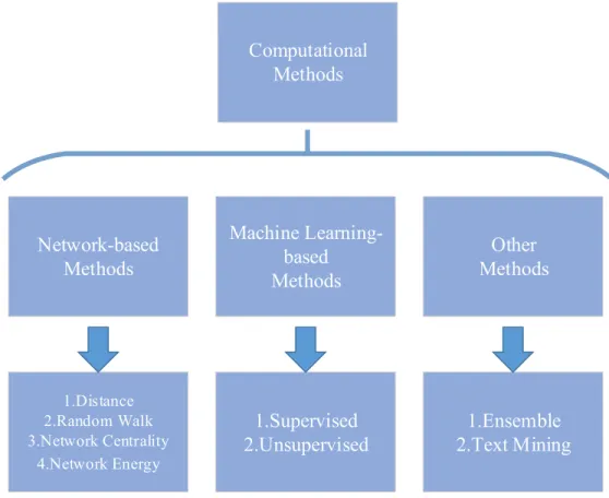
Based on the principles used in the classification, existing methods can be divided into various categories. In [11], the authors have classified computational methods based on three criteria: “type of evidence”, “scope of application” and “type of prediction”. With these criteria scientists can quickly find the methods they need based on their objectives and data at hand. However, methods in each category might vary a lot in terms of their core models, which is inconvenient for researchers who want to improve current models and develop new algorithms. In this review, instead of using these criteria, we focus on the characteristics of computational algorithms and classify them into network-based methods, machine learning-based methods, and other methods. Figure 2.1 shows the details of the classification. We believe that such a classification can help researchers capture the core ideas behind existing algorithms, which might assist them in developing new effective algorithms.

(20)

Computational

Methods

Network-based

Methods

Machine

Learning-based

Methods

Other

Methods

1.Distance 2.Random Walk 3.Network Centrality 4.Network Energy

1.Supervised

2.Unsupervised

1.Ensemble

2.Text Mining

Figure 2.1: Classification of existing computational methods for disease gene prediction.

In the rest of this review, we first discuss existing computational disease gene prediction methods. Then, a few types of frequently used data are described in Section 2.3, as well as the strategies developed for analyzing them. After that, Section 2.4 introduces some evaluation methods. Finally, we conclude with a discussion of the limitations of existing methods and perspectives for developing new algorithms in the future.

2.2 Computational methods

2.2.1 Network-based methods

Based on the ‘guilt by association’ assumption, genes associated with each other may have similar func-tions [14]. Therefore, various types of biomolecular networks which characterize associafunc-tions among genes have been used to predict disease genes. Very briefly, network-based algorithms can be divided into four groups: distance-based methods, random walk-based methods, network energy-based methods, and network centrality-based methods.

(21)

Distance-based methods

Distance-based methods were the first to be developed to predict disease genes. These methods use the length of the shortest path (distance) in biomolecular networks to determine if a gene is disease-associated. Unknown genes (genes that have not been identified as being associated with a certain disease) with a distance smaller than a threshold are predicted as disease-associated. For instance, George et al. developed a method known as CPS which predicted a gene as disease-associated if it was in a disease-related pathway and close to the known disease genes [15]. Snel et al. combined PPI network with disease-associated loci to predict a gene as disease-associated if it was located within these loci, and its neighbors contained known disease genes [16]. Franke et al. used the distance to calculate similarity scores with the Gaussian kernel, and unknown genes with higher similarity scores were predicted as disease-associated [17].

These methods only use local topological structures, and their accuracy is limited. Random walk-based methods have shown that the global topological structure is more valuable for disease gene prediction than local information [18]. Nevertheless, the distance-related evidence is still valuable and has been used to extract features with many machine learning-based methods [19].

Random walk-based methods

To improve the distance-based methods, the random walk is applied to predict disease genes. Even since the first random walk with restart (RWR) algorithm was proposed in [18], it has become one of the state-of-the-art algorithms for disease gene prediction. As a kind of information flow-based algorithm, random walk-based methods propagate the prior information from each node to its nearby nodes in an iterative manner for a predefined number of steps or until convergence. The final value of a node is influenced by the values of its direct neighbors, which in turn are affected by their neighbors. This value also represents the probability of each node being associated with the disease under consideration. Due to its superiority, random walk-based methods have been applied in many other areas as well, including gene function prediction [20] and drug target prediction [21].

Given a disease d, letP0 denote the prior information whereP0(i) = 1 represents genei is known to be associated withdandP0(i) = 0 otherwise. The random walk can be performed by the following equation

Pt+1=W Pt=WtP0, (t≥0) (2.1) whereW is the column normalized adjacency matrix of the PPI network. IfW is a stochastic matrix, this process is equivalent to a random walk on the network. Furthermore, if we allow the random walk to restart in every step with a probabilityr, we can obtain the RWR algorithm as follows:

Pt+1= (1−r)W Pt+rP0 (2.2) wherePtin the steady state would contain the probability of each gene being disease-associated.

(22)

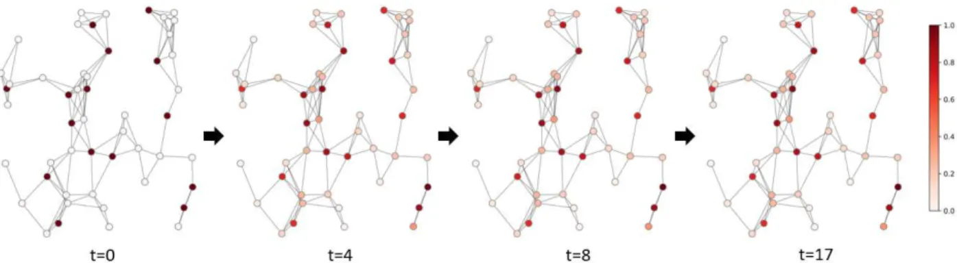
Figure 2.2: Schematic example of a random walk. The network contains 50 nodes (genes), in which 15 of them are disease-associated. Their corresponding entries inP0are equal to 1. The random walk is performed with a restart probability ofr= 0.5, and it reaches a stead state whent= 17.

Figure 2.2 illustrates the process of a random walk which is performed on a randomly generated network with 50 nodes, 15 of which are disease-associated. With a restart probability r = 0.5, the random walk reaches the steady state (Pt+1−Pt<10−6) after 17 rounds of iterations. From the color of the nodes we

can find that the prior information is propagated to the other 35 nodes during the iteration process. K¨ohler et al. first used RWR to predict disease genes in [18]. They also proposed a diffusion kernel method which was the continuous-time analog of RWR. The diffusion kernel of a network was defined by

K=e−βL_{, where} _L₌_D₋_A_{was the Laplacian matrix, D was a diagonal matrix containing the degrees of}

the nodes, A was the adjacency matrix of the network. P was then computed by P=KP0.

RWR and diffusion kernel captured the global topological properties of the network and were superior to the distance-based algorithms. However, K¨ohler et al. only performed RWR on top of a PPI network, andP0 only contained information of known disease-gene associations. To improve the accuracy of the prediction, many researchers started to combine RWR with other types of data.

One strategy is to enhanceP0with information obtained from other types of data. For instance, PRINCE used a logistic function to calculateP0 based on the similarity of diseases [22]. If a gene was associated with a disease which was similar to the disease under consideration, its prior probability would be close to 1. Another strategy is to enrich the PPI network with extra information. For instance, Erten et al. and Le et al. weighted the PPI network with reliabilities calculated from other data sources [23, 24]. Magger et al. built a tissue-specific network and performed PRINCE on it [25].

These methods improved the accuracy of disease-gene prediction. However, they only used PPI networks. To further leverage the potential of random walks, researchers begun to use heterogeneous networks to improve the prediction accuracy.

Heterogeneous networks are networks with multiple types of nodes and edges. The first RWR on het-erogeneous (RWRH) network algorithm was proposed by Li et al. and the network was constructed by combining PPI network, disease gene associations and disease similarity network [26]. RWRH performed much better than the RWR algorithm, and many studies were then conducted to improve it. For instance,

(23)

Luo et al. constructed the heterogeneous network based on a curated PPI network and improved the predic-tion accuracy [27]. Jiang constructed three disease similarity networks and nine gene similarity networks and combined them into 27 heterogeneous networks. Then, RWR was applied on these networks respectively, and a weighted Fisher’s method was used to combine all the propagated values to prioritize disease genes [28]. Valdeolivas et al. constructed a multiplex heterogeneous network in which the same nodes in different heterogeneous networks are connected with each other. This strategy allowed the random walk to transit between different networks, which significantly improved the accuracy of the prediction [29].

Note that heterogeneous networks allow different types of nodes, researchers can also integrate other omics data to construct the network. For instance, Lei et al. constructed a triple heterogeneous network by incorporating long non-coding RNA (lncRNA) into the network. Specifically, lncRNA-lncRNA similarity network, gene-lncRNA associations and lncRNA-disease associations were fused to the traditional heteroge-neous networks [30].

Network centrality-based methods

Centrality characterizes the importance of nodes and edges in a network, which has been widely used in social network analysis [31, 32] and essential protein prediction [33, 34, 35]. However, genes that transcribed to essential proteins are usually not disease-associated [36], and directly applied network centrality to predict disease genes is difficult.

The most successful centralities used in disease gene prediction are feedback centralities, such as Katz centrality and PageRank. These centralities of one node depends on the centralities of its neighbors, which further depends on the centralities of their neighbors. The process of feedback is similar to RWR. In fact, RWR is also known as personalized PageRank [37]. Therefore, methods that use feedback centrality also use similar strategies as random walk-based methods to predict disease genes. For instance, Singh-Blom et al. built a heterogeneous network and used Katz centrality to characterize the possibilities of every disease-gene pairs being associated [38]. Ganegoda et al. also used Katz centrality in their study [39], except that they replaced the PPI network by a tissue-specific network.

Centrality-based methods improve the disease-gene prediction to some extent. However, compared to directly being used to predict disease genes, Centralities are more likely to be used to extract topological features in machine learning-based methods [38, 40, 41, 42, 43].

Network energy-based methods

The network energy-based method was first proposed in [44]. The authors formulated the disease gene prediction problem as a network labeling problem in which disease genes were labeled as 1 while non-disease genes (genes not associated with the disease) were labeled as 0.

Given h genes in a biomolecular network, a set of binary labels x = (x1, x2, . . . , xh) of these genes,

(24)

all possible configurations is a random field. The probability of the configurationxof a random fieldX can be calculated by the Boltzmann distribution [45]

P(x) = 1

Y ·exp(−κH(x)) (2.3)

whereH(x) is the Hamiltonian (energy) of the configurationx,κis a parameter, andY is called the partition function and defined asY =P

x∈Xexp(−κH(x)). From this equation we can find that the true configuration

of the network should have the maximum probability and thus the minimum energy.

Let x[−i] be the set of binary labels of all genes except for gene i in the network. Adopting the Ising model to calculate the Hamiltonian, the following equation can be obtained

P(xi= 1|x[−i],θ˜) =

eα+βNi0+γNi1

eα+βNi0+γNi1+ 1 (2.4) where ˜θ = (α, β, γ) are model parameters. Ni0 andNi1 are the numbers of neighbors with labels 0 and 1 of gene i, respectively. Details of the derivation can be found in [46]. Parameter ˜θ can be estimated by maximizing the posterior distribution ofP(x1, . . . , xn|xn+1, . . . , xn+m) wherexn+1, . . . , xn+m are the labels

of themknown disease genes. Furthermore, ifM networks are available, (2.4) can be generalized as follows

P(xi= 1|x[−i], θ) = exp(V(i)) exp(V(i)) + 1 (2.5) where V(i) =α+ M X m=1 [βm·N_im₀ +γm·N_im₁],

µ = (α, βm, γm) (m = 1, . . . , M) are model parameters. N_im₀ and N_im₁ are the numbers of neighbors with labels 0 and 1 of geneiin them-th network, respectively.

Network energy-based model can be used to integrate multiple biomolecular networks to predict disease genes. In [46], the authors integrated five biomolecular networks and estimatedθwith Gibbs sampling. Later on, they combined graph kernel with their model and proposed a kernel-based algorithm. This strategy allowed the algorithm to use the information between genes and their indirect neighbors since kernel brought similarity information into the network [47]. Having noticed that Eq. (2.4) followed a logistic model where

φi= (1, Ni0, Ni1) was the feature vector and ˜θwas the weight parameter. Parameter ˜θcould be estimated by

a convex optimization problem which was much faster than the original Gibbs-based methods. Ni0andNi1 could also be extended to extract more similar features. Thus, Chen et al. proposed a fast algorithm based on this new strategy and extracted additional featuresN_il₀ and N_il₁ which were the number of the l-order neighbors of genei[48]. This algorithm improved their original running time by more than 20 folds and the performance for more than 10% in terms of the area under the receiver operating characteristic curve.

2.2.2 Machine learning-based methods

Machine learning-based methods formulate disease gene prediction as a binary classification problem where disease genes are predicted as 1 and non-disease genes are predicted as 0. Based on whether known disease

(25)

genes are used in the prediction, machine learning-based methods can be divided into unsupervised methods and supervised methods.

Unsupervised methods

Unsupervised methods identify patterns in dataset without knowing the labels of instances. For disease gene prediction, most unsupervised methods use clustering algorithms to predict disease-associated modules from biomolecular networks. These modules are subnetworks consisting of genes associated with the diseases. The first widely used algorithm, Weighted Gene Correlation Network Analysis (WGCNA), used hierarchical clustering on top of co-expression networks to search disease-associated modules [49]. WGCNA provided an easy-to-use R package, and many studies have used it to identify disease-associated genes [50, 51]. In addition to co-expression networks, researchers also combined co-expression and PPI networks to find disease modules. For instance, Wu et al. weighted a protein functional interaction network with Pearson correlation coefficient (PCC) and applied Markov clustering on this network to predict disease genes [52]. This method allowed the clustering algorithm to leverage the topological properties within the PPI networks.

Although successful, these algorithms mainly used co-expression data to find disease-associated modules, and only a small amount of genes (<20%) in the detected modules are disease-associated [53]. To improve the efficiency, differential co-expression (also known as “guilt by rewiring”) [54] was applied to predict disease modules.

Usually, genes that are differentially co-expressed in different groups of samples are more likely to be disease-associated [55, 56]. Methods based on this assumption construct differential networks in which edges are weighted by the variation of co-expression and apply clustering algorithms on these networks to predict disease genes. For instance, DiffCoEx built an adjacency change matrix based on the co-expression networks of two conditions (case and control). Then, the topological overlap was used to construct a dissimilarity network, and hierarchical clustering was used to find out modules that were differentially co-expressed with the same sets of genes [57]. Another example is EW dmGWAS, which weighted the edges of a PPI network with differential co-expression and nodes of the network withP-values obtained from GWAS data. A seed-growth approach was then used to find subnetworks with the locally maximum proportion of low-P-values and highly rewired edges [58].

Unsupervised methods can be applied to predict disease genes even if a disease has no known associated genes. Since known disease-gene associations are not used in the prediction, their accuracy is usually worse than supervised methods. However, unsupervised methods are still widely used in analyzing biological data, especially gene expression data. One reason is that these algorithms are user-friendly, and do not require complicated data preprocessing. Another reason is that large numbers of gene expression data are available for applying unsupervised methods. Biclustering algorithms and differential co-expression analysis have successfully identified many tissue-specific and cell-type-specific disease-related modules.

(26)

Data 1 Data 2 Data n

...

Feature 1 Feature n

...

Data 1 Data 2 Data n

..

.

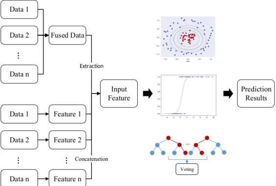
Fused Data Feature 2 Input Feature Extraction Prediction Results ... Voting Concatenation

Figure 2.3: Classic pipeline of supervised machine learning-based methods.

Supervised methods

Supervised methods train a classifier/regressor based on the known disease-gene associations. Figure 2.3 shows the pipeline of most supervised methods. First, the features are either extracted from a fused dataset (e.g. PPI network weighted by gene expression or GWAS data) or concatenated from feature subsets ex-tracted from each type of data. Then, a classifier/regressor, such as biased SVM, logistic regressor and random forest, is trained with these features and used for future prediction. Based on the key ideas of the methods, supervised methods can be further divided to feature-based, deep learning-based and matrix factorization-based methods.

A. Feature-based

Feature-based methods focus on extracting features which characterize the functional similarities of genes. Appropriate data integration is necessary for obtaining discriminative features.

As depicted in Figure 2.3, the features can be extracted from fused data or concatenated from individual features extracted from each type of data. No matter which strategy is chosen, most feature-based methods linearly combine different types of data. For instance, Wu et al. proposed CIPHER, which extracted shortest-path based features from a heterogeneous network [19]. ProDiGe used kernels to calculate gene similarities from each type of data and combined them together by the weighted average of these similarity profiles [3]. PUDI directly concatenated features extracted based on GO, protein domain and a PPI network [41].

(27)

shortest path or degree of the node can capture the topological properties of the entire network. To improve these strategies, researchers started to use multiple types of centralities to extract both local and global topological properties. For instance, Ramadan et al. extracted 13 topological features, most of which were centrality indices, and trained a decision tree to predict disease genes [42]. Luo et al. used closeness centrality and edge clustering coefficient to capture both global and local topological structures from a sample-specific network [43]1_.

Methods using centrality-based features perform better than earlier developed algorithms; however, cen-trality indices are not the best approach for learning network representations. Considering that many algorithms have been developed to learn network embeddings, researchers started to use these algorithms to extract features for disease gene prediction. For instance, Ata et al. proposed an algorithm (Metagraph+) which constructed a metagraph by combining PPI networks and keywords that describe the mechanisms of proteins [59]. In the metagraph, each protein was connected with other proteins and the keywords that de-scribe itself. A matagraph embedding learning algorithm, SymISO [60], was used to extract representations for each protein (gene). Moreover, researchers can also concatenate network embeddings with other types of features to improve prediction accuracy. In [61], Ata et al. proposed N2VKO, which directly extracted fea-tures from PPI networks by node2vec [62], and concatenated these embeddings with feafea-tures extracted based on UniProt annotations. They tested the features with several classifiers and demonstrated that N2VKO performed better than many classic algorithms, such as RWRH, ProDiGe and Metagraph+.

Note that most algorithms extract features from PPI networks using all the known disease-gene asso-ciations. However, Know-GENE proposed by Zhou et al. showed that features extracted with a subset of disease genes were more discriminative than those extracted using all the disease genes [63]. These subset of genes, defined as “Core genes”, were those residing in the largest interacting cluster formed by all the disease genes. Researchers could use this strategy when developing new algorithms.

B. Deep learning-based

Similar to feature-based methods, deep learning-based methods also focus on feature extraction. However, the non-linear activation functions in deep learning models enable an algorithm to learn the non-linear relationships between different types of data, which is different from traditional feature-based methods. For instance, Luo et al. proposed a method which used multimodal deep belief net (DBN) to combine features extracted from different modalities [64]2_{. Specifically, raw features learned based on gene ontology and PPI} networks were fused by a multimodal DBN to learn cross-modality representations, which were further used to predict disease-gene associations. Their evaluation results showed that prediction using cross-modality features were more accurate than original raw features.

In addition to DBN, convolutional neural network (CNN) was also used to predict disease genes. Different

1_{[43] is Chapter 4 from this thesis} 2_{[64] is Chapter 5 from this thesis}

(28)

from image data, gene-related features do not contain spatial information. However, a model known as graph CNN can solve this problem. In this model, the convolution is performed by aggregating information from the neighbors of each node in a graph [65]. This graph can model any biomolecular networks that reveal the functional similarity of genes. In [66], the authors used graph CNN to learn representations from a heterogeneous network. Specifically, raw features extracted for diseases and genes were integrated into the heterogeneous and further learned by graph CNN. Their evaluation results showed that the method performed much better than most classic algorithms, such as inductive matrix completion (IMC) [6] and Katz [38]. C. Matrix factorization-based

Apart from feature-based methods, nonnegative matrix factorization (NMF) has also been used to predict disease genes. Unlike most supervised methods, NMF-based methods can predict disease genes even if the disease under consideration has no known associated genes. Given a disease-gene association matrixA, in which A(i, j) = 1 if disease i and gene j are associated and A(i, j) = 0 otherwise. The general idea is to find a low-rank matrixP =W HT_{, where}_W _∈

Rm×k and H ∈Rn×k are of rankk min(m, n), so that

P ≈A. This problem can be solved by NMF, and matrixP contains the probabilities of every disease-gene pairs being associated. During the factorization, additional information can be integrated into the objective function so that the factorization is in concert with other biological evidence. A typical algorithm was the IMC proposed by Natarajan and Dhillon. The algorithm leveraged gene-related and disease-related features during the factorization, making it possible to integrate multiple types of data [6]. Another example was the probability-based collaborative filtering model (PCFM) proposed by Zeng et al. which used alternating least squares to solve the factorization [7]. In PCFM, disease similarities and gene similarities were used to regularize the objective function, which was a common strategy used by many NMF-based studies.

In addition to classic NMF algorithms, manifold learning can also be used in disease gene prediction. Different from NMF where entries in P denote the probabilities of diseases and genes being associated, manifold learning mapped the diseases and genes onto a lower dimensional manifold and used the geodesic distance between diseases and genes to predict their associations [67, 68]3. Known disease-gene associations are used in the mapping based on the assumption that distance between a disease and its associated genes should be shorter than other non-disease genes. Thus, disease-gene pairs with smaller distance on the lower dimensional manifold are more likely to be associated.

2.2.3 Other methods

Other than the methods discussed in Sections 2.2.2 and 2.2.1, there are also many algorithms that cannot be classified into the previous two categories. One of them is ensemble-based methods which calculate a few ranked lists based on different types of data and outputs the final prediction by fusing all the ranked lists. Different models can be applied when the ranking is calculated on each type of data. A typical

(29)

example is Endeavor, one of the most famous ensemble-based methods, which can analyze 75 data sources and predict associated genes for six species. During its prediction, rankings obtained from each data source were combined by order statistics [69, 70]. Another example was DADA, which proposed five statistical adjustment methods to generate five raw rankings and used the best ranking of each gene as its final ranking [71].

Another type of method is text-based, which used text mining to analyze existing literature and predict disease genes. For different methods, the model might be completely different. For instance, DISEASES calculated a score for each disease-gene pair according to their co-occurrence within the same abstracts and the same sentences [72]. DigSee extracted ten linguistically motivated features and used a Bayesian classifier to identify disease-gene association evidence [73, 74]. Although text-based methods cannot providede novo

prediction (only documented genes can be predicted), their results are useful for disease gene databases, and many databases have used text-based methods to collect disease-gene associations [72, 75, 76].

2.3 Biological data

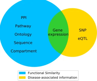
As discussed in Introduction, various types of data have been used to predict disease genes. Figure 2.4 shows several types of widely used evidence in existing algorithms. Some of them characterize the functional similarity of genes, while others directly provide disease-associated information.

2.3.1 Disease-gene associations

The known disease-gene associations are the most significant. These data can be used to predict new disease genes and evaluate the prediction accuracy. Table 2.1 lists six databases that collect disease-gene associations. The first five databases (OMIM, DisGeNET, GAD, CTD, and PsyGeNET) contain genes associated with all kinds of diseases while the last one (COSMIC) mainly collects cancer-associated genes. Among these databases, OMIM is the most frequently used one in the algorithms we reviewed. However, OMIM focuses on Mendelian disorders, and genes associated with complex diseases are not comprehensively collected. An alternative is DisGeNET, which collects disease-gene associations from seven data sources, including CTD and PsyGeNET. This might be a better choice for studies on complex diseases.

In addition, although many algorithms are not specifically designed for cancer, researchers prefer to use cancer to validate their methods. One of the reasons is that many wet-lab studies have been conducted on various types of cancer, which is convenient forde novo validation. Another reason is that different types of cancer are well studied, and the number of known cancer-related genes is larger than other diseases, which is beneficial for training the model, especially for supervised learning methods. For methods that use cancer to evaluate their performance, the Cancer Gene Census project in COSMIC contains the most comprehensive cancer-related genes. Thus, algorithms should use their association data for the prediction.

(30)

PPI

Pathway

Ontology

Sequence

Compartment

SNP

eQTL

Gene

expression

Functional Similarity

Disease-associated information

Figure 2.4: Eight types of evidence valuable for disease gene prediction. The five types of evidence in the left blue circle characterize the functional similarity of genes, and the two types of evidence in the right yellow circle contain disease-associated information. Gene expression in the middle contain both types of information.

Non-disease genes

Along with disease-gene associations, many algorithms require non-disease genes to train their models or evaluate their performance. Unfortunately, no databases contain non-disease genes, and computational methods have to select a set of unknown genes as non-disease genes. The simplest strategy is to randomly select a group of unknown genes as non-disease genes. The number of the selected genes varies depending on the model used for prediction. For weighted models (e.g. biased SVM or weighted random forest), the number of the non-disease genes is usually five to twenty fold higher than the known disease genes. For other models, the size of the positive and negative data should be similar to avoid imbalanced samples. Although the selected genes might be unidentified disease genes, the probability would be small since the number of all disease genes is much less than that of unknown genes. Furthermore, the bootstrap aggregating which improves the stability and accuracy of computational prediction [77] can be used by selecting several groups of non-disease genes and performing the prediction in an ensemble manner.

Additionally, instead of randomly selecting a group of unknown genes, for supervised machine learning-based methods, a better choice is to first define a set of highly potential non-disease genes [reliable negatives (RNs)], then select a subset of genes from RN as negatives. For instance, Luo et al. calculated the similarities of various diseases and used the associated genes of one disease as non-disease genes of the other one for

(31)

Table 2.1: Some commonly used databases of disease-gene associations

Name URL Ref. Latest Update

OMIM https://www.omim.org [80] 01/01/2019 DisGeNET http://www.disgenet.org [81, 76] 01/14/2019 GAD https://geneticassociationdb.nih.gov [82] 08/18/2014 CTD http://ctdbase.org [83] 01/13/2019 PsyGeNET http://www.psygenet.org [84, 85] 09/02/2016 COSMIC https://cancer.sanger.ac.uk [86, 87] 11/13/2018

two dissimilar diseases [78]4_{. This strategy collected a set of RN which enabled the training of a successful} model. However, note that the reasons of different genes not associated with a disease are different. Some of these genes might be passenger genes while others might have completely no function for disease genesis. A set of well defined non-disease genes might be linearly separable from the disease genes, resulting in high prediction accuracy. However, this accuracy does not guarantee the successful prediction of all unknown genes. To solve this issue, Yang et al. proposed a strategy in PUDI which classified unknown genes into four categories: likely positives, likely negatives, reliable negatives, and weak negatives [41]. This strategy allowed the model to be trained with different types of unknown genes, which would enhance its ability in predicting new disease genes.

For network-based and other methods, the artificial linkage interval was frequently used to select non-disease genes [3, 79]. This strategy selects 99 genes that surround a non-disease gene on the chromosome as non-disease genes. During the prediction, each known disease gene and its 99 closest genes are regarded as unknown. Since similar genes tend to cluster in chromosomal neighborhoods, if an algorithm is more accurate in identifying disease genes from its neighbor genes, its performance should be better than the competing algorithms.

2.3.2 PPI network

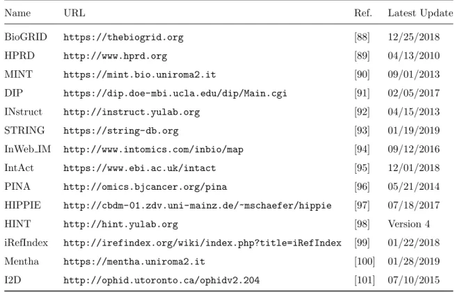
PPI networks are the most widely used data in all three types of algorithms. Usually, proteins are mapped to their corresponding genes to form a gene interaction network. In this section, we will use genes and proteins interchangeably. Right now, many databases are available for researchers to download PPI networks. Table 2.2 summarizes several databases and the date of their latest updates. The first four databases (BioGRID, HPRD, MINT, and DIP) collect PPIs from published literature while the rest ten databases also collect PPIs from other databases. Among these databases, INstruct curates the interactions and constructs a 3D PPI network.

From Table 2.2, we can find that more than half of the databases have not been updated for at least one

(32)

Table 2.2: Some commonly used databases of PPI networks

BioGRID https://thebiogrid.org [88] 12/25/2018 HPRD http://www.hprd.org [89] 04/13/2010 MINT https://mint.bio.uniroma2.it [90] 09/01/2013 DIP https://dip.doe-mbi.ucla.edu/dip/Main.cgi [91] 02/05/2017 INstruct http://instruct.yulab.org [92] 04/15/2013 STRING https://string-db.org [93] 01/19/2019 InWeb IM http://www.intomics.com/inbio/map [94] 09/12/2016 IntAct https://www.ebi.ac.uk/intact [95] 12/01/2018 PINA http://omics.bjcancer.org/pina [96] 05/21/2014 HIPPIE _{http://cbdm-01.zdv.uni-mainz.de/~mschaefer/hippie} [97] 07/18/2017

HINT http://hint.yulab.org [98] Version 4

iRefIndex http://irefindex.org/wiki/index.php?title=iRefIndex [99] 01/22/2018

Mentha https://mentha.uniroma2.it [100] 01/28/2019

I2D http://ophid.utoronto.ca/ophidv2.204 [101] 07/10/2015

year. Meanwhile, since protein interaction is tissue-specific and dynamic, PPI networks downloaded from these databases contain many false positives [4], which significantly affects the accuracy of the prediction, especially for network-based methods. Many approaches have been proposed to improve the quality of the downloaded PPI networks. One of them is to filter out PPIs with low confidence scores. A few databases, such as STRING and InWeb IM, offer confidence scores which represent the reliability of the PPI. PPIs with low confidence scores are usually collected from animal experiment or computational prediction, which can be removed if users need a high-quality network.

2.3.3 Gene expression

Gene expression profiles are the second most popular data for disease gene prediction. Before the widespread use of next-generation sequencing technologies, gene expression data measured by microarray or RNA-seq are the most accessible data to enhance the prediction of disease genes. Although gene expression cannot directly provide association information, the expression pattern of genes in different groups of samples helps us identify disease genes.

Gene expression data can be used to extract features, weight the PPI networks, and build tissue-specific networks. We can also use them to build independent networks, such as co-expression networks [48],

(33)

reg-ulatory networks and differential co-expression networks [78] 5. The datasets of gene expression can be obtained from many platforms, such as the Gene Expression Omnibus (GEO) [102, 103] and Genomic Data Commons (GDC) Data Portal (previously known as TCGA) [104]. Similar to PPI networks, gene expression data suffer from quality issues. No matter how the expression levels are measured (microarray or RNA-seq), preprocessing should be performed to remove low-quality samples and non-expressed genes. Moreover, the data have to be normalized before cross sample analysis, especially for RNA-seq data, which are usually not normalized. Many algorithms have been proposed to normalize the raw RNA-seq count data, and details of their comparison can be found in [105].

Among all the applications of gene expression, co-expression analysis is the most frequently used one. Co-expression patterns, especially differential co-expression, reveal disease-associated properties, and many algorithms have used them to predict disease genes [106]. However, both expression and differential co-expression characterize only a part of the disease gene-related information. Neither of them can solve the problem alone, and gene expression data should be integrated with other types of data when designing a computational method.

2.3.4 Mutation data

Unlike other types of data which mainly provide functional similarity information, mutation data contain the association information between diseases and mutations, which has accelerated the identification of disease genes. Currently, mutation data are obtained from sequencing studies, such as GWAS, Whole Exome Sequencing (WXS) and Target Sequencing (TS).

In typical GWAS, patients and normal controls are genotyped to identify disease-associated single nu-cleotide polymorphisms (SNPs). For each SNP, aP-value calculated from statistical tests is used to represent its likelihood of being disease-associated. These SNPs can be further mapped to their corresponding genes to generate a group of candidate disease genes. Generally, an SNP is mapped to a gene if it is located within the gene sequence or 20 kb upstream or downstream. If multiple SNPs are mapped to the same gene, the most significant SNP (the one with the smallest P-value) would be chosen. Post-GWAS algorithms then combine these candidate disease genes and their mapped P-values with other types of data, such as PPI network, to select a subset of genes as disease genes.

Another type of data that can be obtained from GWAS are the expression quantitative trait loci (eQTL). Mutations in these loci can modulate the expression of genes, which might lead to diseases. Based on the distance between the loci and the genes, eQTL can be divided to cis (close to a gene) and trans (distal to a gene or on different chromosomes). Studies have shown that trans eQTL are more important than cis eQTL for their influence on gene expression [107, 108]. Since eQTL can provide additional disease-related information, algorithms have combined SNPs and eQTL to improve the accuracy of disease gene prediction

(34)

Table 2.3: Some commonly used databases of Pathways

KEGG https://www.genome.jp/kegg [119, 120, 121] 01/01/2019

Reactome https://reactome.org [122] 12/13/2018

WikiPathways https://www.wikipathways.org [123] 01/01/2019 Pathway Commons https://www.pathwaycommons.org [124] 01/28/2019

[109, 110].

Currently, several databases collecting GWAS data are available, such as GWAS catalog [111] and dbSNP [112]. The most popular eQTL database is GTEx Portal. Researchers can also obtain eQTL data of specific tissues from references [113, 114].

In WXS and TS studies, various types of somatic mutations [single nucleotide variants (SNVs), insertions or deletions (indels), etc.] are identified, and computational algorithms can predict disease genes by analyzing their frequency or functional impact. However, unlike GWAS which has been conducted for more than ten years. WXS relies on the next generation sequencing technologies, and mutation data measured from these studies are not always available for all kinds of diseases. Thus, somatic mutation data are not further discussed in this review. Studies about analyzing somatic mutation data can be found in [13].

2.3.5 Pathway

It is well known that disease genes of the same or similar diseases may exist in the same biological module, such as protein complexes [115], and pathways [116]. Therefore, pathways are also valuable for disease gene prediction. Table 2.3 lists a few pathway databases that are commonly used in computational algorithms.

In earlier stages, some computational algorithms regarded unknown genes in the same pathway with the known disease genes as candidates and identified real disease genes from them [15]. Later on, Chen et al. extracted features from a pathway co-exist network in which two genes were connected if they belonged to the same pathway [117, 118]. Currently, pathways are more commonly used to validate thedo novo prediction of the algorithms. The corresponding methods are discussed in Section 2.4.3.

2.3.6 Other types of data

Apart from the widely used data discussed in the previous sections, many other types of data are also useful in predicting disease genes. One of them is ontology data, which includes gene ontology [125, 126] and phenotype ontology [127, 128]. Ontology terms can be described by directed acyclic graphs (DAG) where nodes represent terms while edges represent semantic relations. The major application of gene (phenotype)

(35)

ontology in disease gene prediction is to calculate the similarities among genes (diseases) [129, 64]6. A few algorithms have been proposed to calculate the semantic similarities based on ontology data [130, 131]. We can also extract features from gene ontology data and train machine learning models with them [41, 132]. Moreover, databases like MeSH, also contains disease terms in the form of DAG which can be used to compute disease similarities [133].

Another type of data is subcellular localization, which represents where a protein resides in cells. There are 11 compartments, and two proteins may not interact with each other if they are not localized in the same compartment. Databases such as COMPARTMENTS [134] and LOCATE [135] contain experimentally validated subcellular localization data. Based on our experience, directly using data obtained from these databases and removing protein interactions if two proteins are not in the same compartments might not improve the prediction accuracy, since subcellular localization information is still being identified. A better choice is to weight the PPI networks with the currently available localization data using the strategy proposed in [136, 79].

Finally, protein sequence and domain information are related to the protein functions, which is valuable for disease gene prediction. However, due to their complexity, only a few algorithms have used them in the prediction [137, 41].

2.3.7 Data integration

Each type of data discussed in previous sections characterizes its unique biological properties. To improve the prediction accuracy, it is necessary to properly integrate different types of data so that their shortcomings are compensated. Currently, network-based strategies are most commonly used in integrating multiple types of data.

Network-based

A. Single network-based

Single network-based strategies focus on weighting the PPI network with additional information. Generally, pair-wise measurements, such as correlation coefficients, subcellular localization and gene similarities, can be used to weight the edges of the network, while single gene-related information, such as average expression level,P-values mapped from GWAS data, can be used to weight the nodes of the network.

Additionally, PPI networks can be curated to improve its accuracy. A typical example is to construct tissue-specific networks based on gene expression data. The key idea is to remove a protein interaction if one of the two interacting genes is not expressed in the corresponding tissue. However, it is difficult to determine whether a gene is expressed or not. Earlier method regarded a gene as expressed if its expression level was higher than a threshold [138]. Later on, Ganegoda et al. calculated the PCC of all interacting genes and

Identifying disease-associated genes based on artificial intelligence