Picos: A Hardware Runtime Architecture Support for OmpSs
Fahimeh Yazdanpanaha,b, Carlos ´Alvareza,b, Daniel Jim´enez-Gonz´aleza,b, Rosa M. Badiaa,b,c, Mateo Valeroa,b
aUniversitat Polit`ecnica de Catalunya (UPC), Barcelona 08034, Spain bBarcelona Supercomputing Center (BSC), Barcelona 08034, Spain
cArtificial Intelligence Research Institute (IIIA), Spanish National Research Council (CSIC), Spain
Abstract
OmpSs is a programming model that provides a simple and powerful way of annotating sequential programs to exploit heterogeneity and task parallelism based on runtime data dependency analysis, dataflow scheduling and out-of-order task execution; it has greatly influenced Version 4.0 of the OpenMP standard. The current implementation of OmpSs achieves those capabilities with a pure-software runtime library: Nanos++. Therefore, although powerful and easy to use, the performance benefits of exploiting fine-grained (pico) task parallelism are limited by the software runtime overheads. To overcome this handicap we propose Picos, an implementation of the Task Superscalar (TSS) architecture that provides hardware support to the OmpSs programming model. Picos is a novel hardware dataflow-based task scheduler that dynamically analyses inter-task dependencies and identifies task-level parallelism at run-time. In this paper, we describe the Picos Hardware Design and the latencies of the main functionality of its components, based on the synthesis of their VHDL design. We have implemented a full cycle-accurate simulator based on those latencies to perform a design exploration of the characteristics and number of its components in a reasonable amount of time. Finally, we present a comparison of the Picos and Nanos++runtime performance scalability with a set of real benchmarks. With Picos, a programmer can achieve ideal scalability using aggressive parallel strategies with a large number of fine granularity tasks.
Keywords:
Hardware Implementation, Task Scheduling, Dataflow Execution, Parallel Programming Model, OmpSs, OpenMP
1. Introduction
As computing systems face the end of Dennard scaling [1], or chips hit a power wall because of slowed supply voltage scal-ing [2], multi- and many-cores arise as the main trend in current architectures. Although this approach has allowed chips to keep pace with Moore’s law, it has also introduced new challenges to programmers. Indeed, parallel programming is an issue that is far from being solved and several works have addressed it.
Parallel programming models represent one of the main and more successful trends for solving the programmability issue. Parallel programming models allow the programmer to anno-tate or even fully specify the parallelism of the different se-quences of code within a program. However, this task is often cumbersome as parallel programmers may need to take many details into account in order to avoid stalls and deadlocks that are usual issues when creating parallel programs. New parallel programming models try to leverage these problems by push-ing the complexity of dependency management to the compiler or even the runtime. OmpSs[3] is a programming model that belongs to this last group. It allows programmers to annotate sequential programs with directives that are afterwards used by
Email addresses:[email protected](Fahimeh Yazdanpanah), [email protected](Carlos ´Alvarez),[email protected](Daniel Jim´enez-Gonz´alez),[email protected](Rosa M. Badia),
[email protected](Mateo Valero)
the runtime to ensure correct and as-parallel-as-possible execu-tion. OmpSs has been successful enough to greatly influence the last version (4.0) of the OpenMP standard. Its runtime im-plementation, Nanos++, is a software library that manages the creation of tasks, ordering them according to their dynamically constructed dependency graph, issuing them to execute when ready and, finally, removing them from the dependency graph when finished. Although the Nanos++runtime is optimized, all this work introduces overhead time in each task execution. This overhead influences the overall application performance when approaching fine-grain parallelism with a large number of tasks. The Task Superscalar [4] architecture was the first one to ad-dress this problem, proposing a decoupled model in which dif-ferent finite state machines (modules) manage the most cum-bersome functionalities of the runtime. The first implementa-tion of the Task Superscalar architecture, the Hardware Task Superscalar, has already demonstrated high potential [5]. In this paper we present Picos, a highly evolved hardware imple-mentation of the Task Superscalar architecture designed in the context of the TERAFLUX project (www.teraflux.eu), and we perform a full study of its capabilities and resource necessi-ties. The main contributions of the paper are:
• The Picos hardware design: a new hardware implemen-tation of Task Superscalar architecture with a new opera-tional flow.
• Latency information of each Picos module, based on the synthesis of the VHDL code.
Preprint submitted to Future Generation Computing Systems December 31, 2014
© 2015. This manuscript version is made available under the CC-BY-NC-ND 4.0 license
http://creativecommons.org/licenses/by-nc-nd/4.0/
• A detailed execution analysis of a set of real benchmarks on a Picos-based system.
• A cycle-accurate simulator based on the latency informa-tion obtained. This simulator is used to perform a design exploration of Picos that leads to near optimum results for different sizes (number of cores) of computing systems.
• A comparison analysis of the scalability of Nanos++ run-time, a real pure software implementation, and Picos. The rest of this paper is organized as follows: Section 2 de-scribes the operational flow and the main modules of the Pi-cos Hardware Design; in Section 3 we present the experimental setup used in Section 4, where a full space design exploration of the Picos hardware is shown. Results are shown in Section 5. Section 6 reviews the Related work, and Section 7 concludes. 2. The Picos Hardware
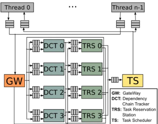
Picos hardware is a major revision of the Hardware Task Su-perscalar architecture with several improvements in its work-flow. The main improvements are related with architectural changes to add support to nested tasks, better memory manage-ment and faster task dispatching. Figure 1 shows the organiza-tion of a computing system that includes the Picos hardware. It consists of a many-core with any number of threads that send two types of task information to the Picos hardware: (1) the dependency information of new tasks, and (2) the notification of ending a task. The Picos hardware consists of one gateway (GW), one or more Dependence Chain Trackers (DCT), one or more Task Reservation Stations (TRS) and one Task Scheduler (TS). All these components work together in parallel in order to build the dynamic task dependency graph and generate a list of ready tasks that are sent back to the threads to be executed. The connections between the modules are decoupled by FIFO queues that are interconnected by arbiter modules (not drawn in Figure 1 for clarity). There is one arbiter module between the output queues of one type of module and the input queues of a different type of module (for example, one arbiter reads from a single output queue from the GW and writes to one of the input queues of the appropiate TRS).
GW
TS
TRS 0 TRS 0 TRS 1 TRS 2 TRS 0 TRS 3 DCT 0 DCT 1 DCT 3 DCT 2 Thread n-1 Thread 0...
GW: GateWay DCT: Dependency Chain Tracker TRS: Task Reservation Station TS: Task SchedulerFigure 1: Computing system with Picos pipeline hardware.
2.1. Operational Flow Overview
Once a thread reaches a task creation it creates a new task descriptor that is basically a memory structure containing the necessary information for the new task to be executed. This information mainly includes the address of the task code to be executed and the address of all its dependencies with their direc-tions (input, output, input and output - inout, or direct for imme-diate values). Once this descriptor is created, it is sent to the Pi-cos hardware that reads its information and stores the data of the corresponding task until all its dependencies are fulfilled. For the first task created, all its dependencies are ready because all its input and inout dependencies are already in memory. How-ever, the most common case is that a task has to wait until one or more of its dependencies become ready after other tasks finish. The information (finishing messages) about those finished tasks is sent to the Picos hardware by the threads that execute those tasks. With this finishing message Picos will delete the corre-sponding descriptor in the system and proceed to mark as ready all the task dependencies that may be waiting for the dependen-cies of the just finished task. The Picos hardware will then try to send the new ready task/s to be executed. This entails send-ing the descriptor to the TS, which will make it available to all the threads in the system. When one thread that is not busy re-alizes that a new descriptor is available it starts executing the corresponding task. If a task creates new tasks, new descriptors are created and the dependency information is sent to Picos as explained above.
2.2. Picos Modules
The GateWay (GW)is a simple selector that reads the mes-sages (new task and finishing task mesmes-sages) that arrive to the system and sends them to the associated module. If the mes-sage is a new task, the GW reads the Task ID and the number of dependencies and sends this information in a packet to the cor-responding TRS. Each dependency is then read and sent to the associated DCT with a packet containing the following infor-mation: address and direction of the dependency, and the task related identifiers (TRS destination, slot position in the TRS, and dependence position inside the task). Therefore, to pro-cess the new task message, the GW needs two items of infor-mation: an empty slot in the TRS modules, and the DCT in which the dependence information should be stored. The selec-tion of the TRS is simply done by using a TRS identifier and a TRS free slot previously read from a queue that comes from the TRS modules. As we will see, each TRS sends a packet with this information to the GW as soon as it has an empty slot. On the other hand, the DCT associated with each dependence is computed directly from the dependence address with a hash function that should be properly selected to balance the load be-tween all the DCTs. If the message is a finishing task message, the GW only needs to forward that information to a TRS. In this case, the TRS identifier and the task slot position are pro-vided by the packet received from the thread that notifies that the task is finished, this thread having previously received that information with the task ready packet (as explained below).
The Task Reservation Station (TRS)is the module that man-ages all the processes related to the in-flight tasks. To this end,
it has a Task Memory (TM) that is an indexed memory in which each TRS stores all the information about the tasks and the readiness of their dependencies. A TRS may receive packets from the GW, the DCTs, and the TRSs. When a packet from the GW arrives at the TRS with information about a new task, the TRS stores it in the slot specified by the packet and then looks for a new free slot and sends it to the GW (which will use it to allocate a new incoming task, as explained above). The TRS will then wait (or perform other processes) for all the de-pendencies of the task to be ready before sending it to execute. A packet coming to the TRS from the DCT or TRS modules (as seen in Figure 1 they share the network) can have two ob-jectives: (1) to update information about a dependence in order to create a chain of dependencies, and (2) to notify that a de-pendence is now ready. In the first case, the TRS only saves the information in the appropriate slot. In the second case, the TRS should update the information, send a packet to the next instance (if it exists) of this version of the dependence and, if all the dependencies of the task updated are now ready, mark the task as ready for execution. In addition, the TRS periodically (i.e. when it is not performing other actions) checks if there are empty slots in the queue to the TS. In this case, the TRS picks an available ready task and sends it to execute. Finally, TRS may receive a packet from the GW informing it that a task has finished. In this case the TRS parses each of the dependencies of the task and sends one packet (per dependence) to the associ-ated DCT, informing it that this instance of the dependence has finished. After that, the TRS frees the slot and, if there were no previous free slots, it sends the associated message with the new free slot to the GW.
The Dependence Chain Tracker (DCT) manages all the
de-pendencies in the system. The dependence information is stored in two different memories: the Dependence Memory (DM) and the Version Memory (VM). DM is indexed by a hash function of the initial dependence address and stores the basic depen-dence information and a pointer to the last version of each de-pendence. We call the ”version of a dependence” every output instance of the dependence and all subsequent input instances (i.e. a producer and all its consumers). Version information is stored in the VM, which keeps one entry for every version of the dependence where the TRS address of the last consumer of this version of the dependence is stored, and also the TRS ad-dress of the producer of the next version, should it exist. When the DCT receives a packet from the GW with a new dependence instance entering the system, it searches for the dependence in the DM. If the dependence is not found, the DCT creates an entry for it both in DM and VM. A packet specifying that the dependence is ready is then sent together with its VM address to the corresponding TRS. Otherwise, when a dependence in-stance is found in the DM, two main possibilities exist: either the dependence has an input direction (i.e. it is a consumer) or it has an output or inout direction (i.e. it is a producer). In the first case the dependence is added to the dependency chain in its last version and a packet to the TRS is sent with the dependency information (the version may or may not be ready). In the sec-ond case, a new version should be created and all memories are correspondingly updated (the DM should now point to the new
version entry and the previous VM entry now includes the TM address of this producer). In this case, a packet is sent to the TRS specifying that the dependence is not ready and the chain information is stored in the TRS. In addition to keeping track of new dependencies, the DCT also updates its information when the TRS, on completion of task, sends a packet releasing a de-pendence instance. When the DCT receives such a packet it updates the corresponding version, and if a new dependence version is ready it sends a packet to the TRS that stores it. Fur-thermore, if the dependence instance was the last of a version, the entry in the VM is deleted. If it was the last dependence instance, the entry in the DM is also deleted.
The Task Scheduler (TS)is a simple dispatcher of tasks. As soon as it receives a ready task, it searches for an available thread and forwards the descriptor associated to the task to that thread. More complex scheduling patterns can be implemented in this module if, for example, the memory accessed by every task is taken into account, but the exploration of these memory conscious scheduling techniques is beyond the scope of this pa-per and remains as subject for future work.
2.3. Picos hardware latencies
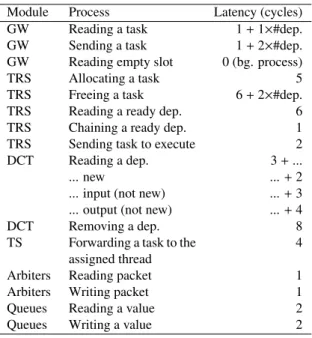
To obtain the Picos hardware latencies we have undertaken a full VHDL implementation of all the modules in the Picos hardware and synthesized them targeting a Virtex-7 device. With this information we have obtained the exact cycles that the finite-state machine (FSM) of every module in the design uses in order to perform every assigned functionality. Table 1 shows the set of latencies corresponding to synthesis of the main functionality of the Picos hardware modules. The laten-cies shown are calculated assuming that everything (for exam-ple the queues) is ready, otherwise the number of cycles spent waiting for an available resource should be added. In addition, the queues have a simple implementation that does not allow them to be read from and written to at the same time. With this implementation, the first cycle in the process of writing from/reading to/from a queue is used to reserve the slot, while the second cycle performs the action. The cycles used to inter-act with the queues are in addition to the cycles specified and should be added for every packet that any module has to send. With this information, we have built a cycle-accurate simulator that exactly replicates the hardware design. The software sim-ulator allows us to fully explore the optimum design point of the modules in terms of number of modules and memory sizes that cannot at present be synthesizable in a real FPGA. It also allows us to implement accurate simulation of complex behav-ior patterns like thoses by nested tasks or by a large number of modules, as well as detecting their bottlenecks and thereby correcting them.
2.4. Design issues
The modular design of Picos introduces challenges that an integrated design may not pose. The main problem sources in this kind of design are the unexpected effects that arise from the interaction of simple behaviors in the modules. In particular, the Finite State Machines in the modules have undergone sev-eral redesign cycles to avoid deadlocks and to minimize stalls.
Module Process Latency (cycles) GW Reading a task 1+1×#dep. GW Sending a task 1+2×#dep. GW Reading empty slot 0 (bg. process)
TRS Allocating a task 5
TRS Freeing a task 6+2×#dep. TRS Reading a ready dep. 6 TRS Chaining a ready dep. 1 TRS Sending task to execute 2 DCT Reading a dep. 3+...
... new ...+2
... input (not new) ...+3 ... output (not new) ...+4
DCT Removing a dep. 8
TS Forwarding a task to the assigned thread
4 Arbiters Reading packet 1 Arbiters Writing packet 1
Queues Reading a value 2
Queues Writing a value 2
Table 1: Modules latencies.
Although a complete description of all the details of the design is beyond the scope of this paper we believe that it is interest-ing to highlight the main points that allow the system to work properly and how they have influenced the design.
The key point that makes the modules work together is the fact that the only module that can stall is the TS. If the TS stalls, it means that all the threads are busy and the system sim-ply waits for them to finish. The GW cannot stall as the system has to wait for tasks to finish. This means that the finished task messages use a different queue than the new task messages and that if a task cannot be issued (due to contention in the TM or in the DCT memories) the GW stores it internally and contin-ues processing finished tasks. The same behavior occurs in the DCTs. If any of the DCT memories are full, the DCT stops processing new dependencies but continues processing packets (releasing dependencies) from the TRSs.
The TRSs have the most complicated behavior. Basically the TRSs may deadlock for two reasons: the first one is that they try to send a ready task to execute but all the threads are busy. This can be solved simply by keeping a bit information for every ready task to indicate that it has not yet been sent for execution yet. After verifying that there is at least one empty execution slot, the TRS reserves it and sends the task to execute. The other source of deadlock is a finished task; a finished task means that the TRS should cycle through all the dependencies in the task, sending messages to the associated DCTs. The deadlock occurs when the DCT follows those messages trying to awake other tasks in other (or the same) TRSs. If two or more TRSs are doing the same thing at the same time (which happens often) a deadlock may occur. In order to prevent this from happenning, the queues from the TRSs to the DCTs are slightly different than the others in the system. Their minimum size is equal to the maximum number of dependencies per task (15), and when fewer than this number of slots in the queue are empty, the TRS does not process finished tasks messages but continues to do other work.
Finally, the memories are a further key design point; although they are not critical from the point of view of reliance, a wrong approach would result in low performance (due to increased access times) and would also probably lead to a lot of wasted resources in the form of redundant data. Table 2 shows the the number of entries per slot for every memory in the system, and the information stored in each entry with its size in bits in our final design (explained below in detail in Section 4).
With the specified memory entry sizes and the data obtained in Section 4, all the memories in the system would amount to a total of: 58.5 KBytes (the TM), 21 KBytes (the DM) and 11,75 KBytes (the VM), distributed in 12 small memories capable of managing up to 1024 in-flight tasks. This size can be further re-duced by optimizing the TM, which is the largest memory in the system. Every entry in the TM uses 6 slots: 1 to manage task information and the other 5 to store information about its de-pendencies (3 dede-pendencies per slot). As most tasks have only a small number of dependencies, making a dynamic assignment of slots 2 to 6 may result in a reduction of this memory to a size of only 19.5 KBytes with the same results. This memory would be able to store up to 1024 in-flight tasks with up to 3 dependen-cies each or 341 tasks with 15 dependendependen-cies each. In this case the total amount of memory in all the modules in the system would be only 52.25 KBytes.
Another critical point about the memories is the DM design, because its behavior is critical to the system performance. A full DM entry that is required for a new dependence means that the system would stall for a long time even if other entries are empty. To alleviate this problem and reduce the effects of cor-ner access patterns, an Inverse Victim-Cache-like mechanism has been used. Should one entry be full, with this mechanism the DCT searches for a space in the next entry. This mecha-nism, although slower than doubling the associativity, uses al-most less than half the resources and provides similar system performance results.
3. Experimental setup
In order to evaluate the capabilities of the Picos hardware, we selected a group of real applications as shown in Table 3. All the benchmarks can be obtained from the BSC Application Reposi-tory (BAR,https://pm.bsc.es/projects/bar). The name of each benchmark is shown, as well as the configuration value used to obtain the trace for the full cycle-accurate simulator; the number task instance executions that it includes; the average length in cycles of the tasks; the maximum and the minimum task sizes; the average number of dependencies per task; the av-erage distance between two consecutive tasks and the number of cycles of the sequential execution in which the trace was obtained. As may be seen in Table 3, the real applications used are Cholesky, Heat (using Gauss-Seidel algorithm), LU and Sparse-LU, all of which are standard implementations that include OmpSs pragmas to annotate where tasks can be created and their dependencies. The traces were obtained by executing the applications sequentially and measuring the time at which each task would be created, as well as the time spent in its ex-ecution and its real dependence information. The configuration
Memory (bits) Field 1 Field 2 Field 3 Field 4 Field 5 Field 6 Field 7 TM Slot 1
(74+4)
Valid Bit (1) Task desc. (64) # dep. (4) # not ready dep. (4) In execution (1) Void (4) – TM Slot 2-6
(3×26)
Dep. VM ad-dress (9)
Dep. eORT id. (2)
Chain dep. (1) TM chain address (8)
TRS chain (2) Chain Dep. (4) – DM (84) Valid Bit (1) Dep. addr. (64) Last ver. addr. (9) Dep. instances (10) – – – VM (47) Version Ready (1) DM dep. entry (6) Consumers exist (1) Last consumer TRS addr. (2+8+4) Next producer exists (1) Next producer TRS addr. (2+8+4) Version instances (10) Table 2: System memories characteristics.
Application Chol. Heat LU Sp-LU Input Conf. 100-2 256-32 256-1 64-8 # of task instances 22100 1025 32896 11472 Avg. task size (cycles) 778 1116 1970 9835 Max task size (cycles) 84704 3124 229924 147128 Min task size (cycles) 416 24 488 3344 Avg. # deps. per task 2.88 4.99 2 2.9 Avg. task dist. (cycles) 31.06 39.63 24.78 139.06 Seq. execution cycles 19.9M 1.2M 114.4M 65.6M
Table 3: Application characteristics.
parameters of the benchmarks were chosen by seeking to obtain executions that generate several fine-grained tasks. The execu-tion time obtained for the given problem size was not a concern in this regard, as we were interested in measuring the ability of the hardware to manage the tasks and not in accelerating the applications.
For the real software run-time system results of OmpSs ap-plications, we used the same task decomposition strategy. The OmpSs implementation employed is based on Mercurium 1.99 and Nanos 0.7a runtime system. The applications were exe-cuted (sequentially and in parallel) in a shared memory machine node with 2 NUMA nodes with 1 socket each. Each socket is a Xeon E5645 with 6 cores each at 2.4 GHz. The system amounts to a total of 24 GB of RAM Memory. The L1 memories (data and instructions) have 32 KB and the L2 has 256 KB per core. The system also has a shared L3 (for each processor) of 12 MB.
4. Space design exploration
In this section, a deep-space design exploration of the Picos hardware it presented. The main goal is to explore the amount of resources required in order to be able to fully exploit current and future many-core designs.
4.1. Picos for High Performance Computing
To start our space design exploration, we selected a very large configuration of the Picos hardware system with more-than-enough resources (number of DCT and TRS modules and their memory sizes), as presented in Table 4. For each configuration parameter, the more-than-enough resources number is selected in such a way that the time results of the system will be the same even if the value is halved. Due to space constraints, we do not show all the experimental analysis performed to obtain the numbers in the table. The results of our preliminary space design exploration are shown in Figure 2, where the Y-Axis shows the speed up over the sequential execution of each of the benchmarks presented in previous section, and the X-Axis
shows the number of processors in the system. Speed-up results range from 11×to 56×, depending on the benchmark, and show that 256 processors are enough to obtain the upper limit of the achievable speed-up with our design. Unless otherwise stated, from now on we will use 256 processors in our space design ex-ploration. It is noteworthy that task scheduling, communication and management overheads have no visible impact on scalabil-ity. This is due to two reasons: first, for all those tasks that do not belong to the critical path of the application, overheads are completely overlapped with the execution of the tasks. Second, for those tasks in the critical path, the non-overlapped hardware overhead is negligible: around 75 cycles per task. For instance, in Figure 2, the application with the shortest tasks, Cholesky, with a critical path of 267 tasks out of 22Ktasks, has a non-overlapped overhead of only 20K cycles, while its sequential execution takes nearly 20Mcycles.
Parameter Value Meaning
# TRS 32 Number of TRS modules TM entries 16K Number in-flight tasks per TRS # DCT 32 Number of DCT modules DM assoc. 16 Associativity of Dep. Memory DM entries 16K Number of dependencies that the
system can keep per DCT
VM entries 16K Number of versions that the system can keep per DCT
Table 4: Picos near-unlimited configuration.
1 2 4 8 16 32 64 128 256 512 1024 2048 # cores 0 20 40 60 Speed-up Chol. Heat LU Sp-LU
Figure 2: Speed-up obtained as a function of the number of processors with more-than-enough resources.
TRS parameter configuration
Once we have obtained an upper limit to our design results, we can reduce the number of resources in order to obtain a con-figuration with an affordable amount of resources suitable for HPC systems with 256 processors. First of all, we show the effect of changing the number of entries in the TRS memory (that is, limiting the maximum number of in-flight tasks that the system supports) when Picos has only one TRS. All the other
parameters are maintained, as in the more-than-enough config-uration. The results are shown in Figure 3, where the Y-Axis shows the speed up over the sequential execution as a function of the number of entries in the Task Memory (X-Axis). In this figure one may observe two interesting effects: the first is that, for the selected traces, 512 in-flight tasks seem enough when we have only one TRS. The second observation is that the speed-ups decrease when compared to those in Figure 2 due to the effect of having only one TRS module in the system. This oc-curs, in particular, for the Cholesky benchmark, while for other benchmarks the speed-ups remain very similar to previous re-sults. Regardless of TM size, the time that the TRS uses to pro-cess the tasks may become the bottleneck of the system. This can be solved by increasing the number of modules of Picos hardware, thereby hiding the latency of the TRS processes.
8 16 32 64 128 256 512 1024 2048 4096 8192 16384 # TM entries 0 20 40 60 Speed-up Chol. Heat LU Sp-LU
Figure 3: Speed-up obtained as a function of the number of Task Memory en-tries.
Table 5 shows how changing the number of TRSs and their memory size influences the number of execution cycles for the Cholesky application. As can be seen in the table, the opti-mum design point is to have 8 TRS modules with the capac-ity to store 512 tasks each (for a total of 4K in-flight tasks), for the Cholesky benchmark. However, this configuration is only ideal for the specific case of Cholesky and presents seri-ous drawbacks from the hardware resources point of view: 8 TRS modules represent a large interconnection network and, furthermore, as explained in Section 2.4, 4K in-flight tasks de-mand at least 80 KBytes of memory storage for the tasks and more space in the other memories, which should be scaled ac-cordingly. Taking into account the results in Figure 3 for all the benchmarks and the hardware resource requirements of a 8 TRSs configuration, we have limited the selected prototype to 4 TRSs, each with a 256-entry TM, thereby reducing the inter-connection network and memory requirements, while guaran-teeing high speed-up.
DCT parameters configuration
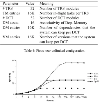
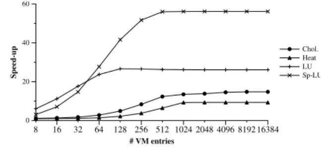
DCT modules keep track of the dependency chain, and in or-der to do so they have to store not only all the dependencies of all the tasks in the DM but also all the versions of those de-pendencies (the different values that the dependency may have due to the different in-flight tasks that produce this value) in the VM. For the VM, the only parameter that may influence the performance of the design is the capacity of the VM (#entries), since a new version can be assigned to any empty entry. Fig-ure 4 shows the speed-up obtained for each benchmark when
TM entries 1 TRS 2 TRSs 4 TRSs 8 TRSs 16 TRSs 8 1.52 2.14 3.36 5.56 9.38 16 2.12 3.35 5.55 9.37 15.10 32 3.31 5.50 9.33 15.07 21.61 64 5.30 9.08 14.99 21.56 23.74 128 8.06 13.78 21.34 23.77 24.60 256 10.03 17.11 23.45 24.59 25.32 512 10.51 17.69 23.97 25.31 25.32 1024 10.60 17.91 24.92 25.31 25.32 2048 10.77 18.33 25.30 25.31 25.32 4096 10.97 18.61 25.30 25.31 25.32 Table 5: Speed-up of Cholesky application as a function of number of TRS modules and their memory size.
the number of entries is modified and we have only one DCT module (in this graph the number of TRSs is 32). As it can be seen in the graph, as in the case of the TM, the Cholesky appli-cation is the most demanding one, needing 4096 entries in the VM to achieve the peak performance. Considering that number of entries, in Figure 5 we show how changing the number of DCT modules affects the speed-up when the total VM is main-tained constant and the Dependency Memory (DM) is kept at its more-than-enough value. In particular, one may observe that 4 DCTs with 1024 entries each (4096 entries in total) reaches the upper performance limit.
8 16 32 64 128 256 512 1024 2048 4096 8192 16384 # VM entries 0 20 40 60 Speed-up Chol. Heat LU Sp-LU
Figure 4: Speed-up obtained as a function of the number of Version Memory entries. 1 2 4 8 16 32 # DCT modules 0 20 40 60 Speed-up Chol. Heat LU Sp-LU
Figure 5: Speed-up obtained as a function of the number of DCT modules.
The Dependency Memory (DM) is the key element in the DCT module. It keeps track of all the dependencies of all the in-flight tasks in the system. When a dependency enters the system, it should determine efficiently whether or not the de-pendency is new and update its meta-data accordingly. As the latency of this search is critical, the ideal way to store the depen-dency information would be in a direct access memory. How-ever, the DM is not a cache, and when a block in the dependence
memory is full the system cannot flush the old entry. Instead, it should stall and wait (perhaps for quite a while) until another dependence that is using the same entry is no longer live. For this reason, an associative memory and a more complex hash function (Pearson-like hash) than the usual one (addresses less significant bits - LSB in Figure 6) is used.
Figure 6 shows the effect of this improved hash function on the speed-up obtained for the Cholesky benchmark as a function of the number of entries in the DM. As may be observed, the improved hash function a has better speed-up for all the cases, and from another point of view allows the system to obtain the same results with smaller DMs. Other results presented in this section use the improved hash.
8 16 32 64 128 256 512 1024 2048 4096 8192 16384 # DM entries 0 10 20 30 Speed-up LSB Hash Improved Hash
Figure 6: Speed-up obtained as a function of the DM entries with and without an improved hash for Cholesky application.
The selected memory associativity is also crucial for perfor-mance. As stated above, the ideal solution would be a full asso-ciative DM, but as this is not possible in a real environment we have studied the effect of having different associativities. With the improved hash shown in Figure 6, 8-way has been selected as sufficient to provide good performance results while ensuring that the resources used are affordable.
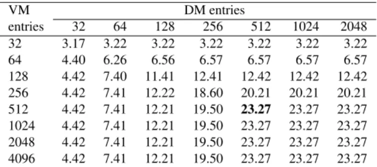
Finally, with the selected hash and memory associativity, we conducted a combined-space exploration of the sizes of both DCT memories (DM and VM). The results in speed-up cycles for a different number of memory entries for the Cholesky ap-plication are shown in Table 6. The number of DM and VM entries in this Table is per DCT, and a total of 4 DCTs were used for obtaining those results, as deduced above. As can be seen, the previously selected 1024 entries for the VM are more than enough, and the correct design point for this benchmark is 512 entries in the VM of each DCT and 64 8-way (512) en-tries for the DM. While this value is not the maximum for each benchmark, it is very close to the upper limit for all benchmarks and constitutes an affordable amount of memory (3 KB the VM and 5.25 KB the DM) in each DCT module.
VM DM entries entries 32 64 128 256 512 1024 2048 32 3.17 3.22 3.22 3.22 3.22 3.22 3.22 64 4.40 6.26 6.56 6.57 6.57 6.57 6.57 128 4.42 7.40 11.41 12.41 12.42 12.42 12.42 256 4.42 7.41 12.22 18.60 20.21 20.21 20.21 512 4.42 7.41 12.21 19.50 23.27 23.27 23.27 1024 4.42 7.41 12.21 19.50 23.27 23.27 23.27 2048 4.42 7.41 12.21 19.50 23.27 23.27 23.27 4096 4.42 7.41 12.21 19.50 23.27 23.27 23.27 Table 6: Speed-up obtained for the Cholesky application as a function of the size of both DCT module memories.
Our last experiment in the space design exploration consists of a crosscheck of the obtained values. We evaluated the sys-tem by changing the number of modules, but maintaining the total amount of memory. The results of this experiment can be seen in Figure 7, which shows that it is necessary to have at least 4 TRS and 4 DCT modules to achieve the upper per-formance limit of the explored system. One may also see that more modules does not help to improve this performance. This is because four modules are enough to exploit the parallelism found in those benchmarks, and any increase in this number only results in a more complex network. Note however that doubling the number of modules halves the memory in each module. This has no influence on the capacity of the system in terms of tasks, since TM is always fully occupied if there are enough tasks, but as dependences can only be stored in the as-signed DCT, halving their memories may sometimes give rise to stalls if their occupancy is not perfectly balanced.
Chol. Heat LU Sp-LU
# modules 0 20 40 60 Speed-up 2 DCTs, 2 TRSs 4 DCTs, 4 TRSs 8 DCTs, 8 TRSs
Figure 7: Effect of changing the number of modules maintaining the sizes of the memories.
In conclusion, our proposed configuration for a Picos Hard-ware machine is composed of 10 modules: 1 Gateway, 4 TRSs, 4 DCTs and 1 TS. Each TRS has a 256-entry TM. Each DCT module has 2 memories: the VM is an indexed array of 512 en-tries while the DM is an 8-way set associative memory with 64 entries (also amounting to a total of 512 entries). In Section 5, we compare the performance results for the set of benchmarks in the selected design to the those that can be obtained with the software runtime as well as to the ideal ones.
4.2. Simple Picos for small multicores
1 2 4 8 16 32 64 128 256 # cores 0 5 10 15 Speed-up 52.25 KB 26.1 KB 13 KB 6.5 KB 3.3 KB 1.65 KB
Figure 8: Speedups obtained with only one TRS and one DCT modules when changing the memory sizes.
In addition to our previous design space exploration target-ing applications that can scale up to 256 processors, we wish to select a more simple Picos hardware design capable of manag-ing small multicores. In order to conduct this exploration we selected an initial configuration of Picos that has only one TRS and one DCT module and configured them with an amount of
memory equal to the total amount in our previous selected de-sign. We obtained the speed-ups that this design can achieve when a variable number of processors is used. We then reduced all the memories by half and repeated the experiment. Fig-ure 8 shows the results obtained for the Cholesky application by means of this experiment. Results for the other benchmarks show a similar behavior. As one may see in this Figure, it is necessary to have only a quarter of the total system memory of our previous configuration to obtain virtually the same re-sults. This means that our minimum configuration is composed of only 4 modules (1 Gateway, 1 TRS, 1 DCT and 1 TS) and each module has exactly the same memory as in our previously selected configuration.
5. Results
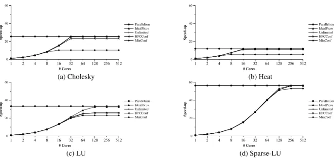
In order to form a good idea of how well our proposed fi-nal systems behave, we evaluated them with a different num-ber of processors, comparing the speedups obtained to a set of control configurations. For each of the benchmarks, Figure 9 shows the maximum speedup that can be obtained with the chosen parallelization strategy (Parallelism=T1/T∞, where T1 is the sequential time andT∞ is the execution time of the
critical path in the parallel execution, with infinite resources) of a given benchmark. Figure 9 also shows the results that would be obtained with a Picos hardware that uses 0 cycles to process any packet (IdealPicos); the results obtained with our previously mentioned Picos near-unlimited configuration (Un-limited); the selected configuration for big systems (HPCConf) in Section 4.1, and the selected minimum configuration (Min-Conf) in Section 4.2.
As one may observe in Figure 9, the selected HPCConf per-formance is almost the same as the near-unlimited one for all the benchmarks. Only in the case of Cholesky can a small slow-down be appreciated as a trade-offof downsizing the resources. As stated in Section 4.2, one can also see that for systems with a small number of processors (up to 8) a minimum configuration (MinConf) is able to keep pace, and thus, it would be both suffi -cient and affordable for implementation in embedded systems.
A comparison of the results in Figure 9 with the maximum parallelism (Parallelism) shows that the implementable Pi-cos hardware can extract all the possible parallelism for three of the four benchmarks. The only exception is for the LU appli-cation, in which maximum speedup with the ideal (impossible) implementation of Picos (IdealPicos) can be obtained, but not with the current one (HPCConf) or even with the near-unlimited (Unlimited). We believe that the difference in performance here is due to the large dependency chains of consumers (255 for each producer) created by the LU application. Awakening 255 consumers means creating a sequential chain of 255 packets between the TRSs, and thus when the last consumer is awak-ened several cycles have been wasted. As an improvement we propose a system that simply creates a new version of a depen-dence when several consumers are detected. This new version awakens at the same time as the original one and splits the chain of packets into two different and parallel chains. However, we
have not implemented this improvement, since with more re-alistic task sizes this behavior will disappear and be hidden by the longer task execution times, as can be seen below in Sec-tion 5.1.
5.1. Comparison with the software alternative
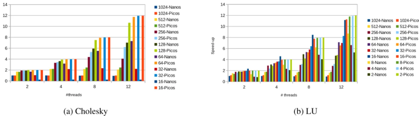
Figure 10 provides a comparison of the benchmark per-formances when using HPCConf and the performance of the OmpSs benchmark versions using Nanos++ runtime for Cholesky and LU problems. OmpSs results are for a machine with 12 cores at 2.4 GHz (see Section 3). The Y-axis in this Figure indicates the speed-ups obtained against the sequential execution when we change the number of threads (X-axis) and the parallel approach (the block size). The executions shown in each graph solve the same problem: a Cholesky and a LU application for a 2048 problem size (matrix), but with dif-ferent block sizes (the different bars are labeled with the se-lected block size) with Nanos++(Nanos bars) and Picos hard-ware (Picos bars). To avoid the variability of comparing dif-ferent executions, all the tests were performed three times and the best results were chosen. Furthermore, it is important to note that while Nanos++real executions are influenced by the parallel memory behavior of the application, Picos results are based on a sequential execution that may exhibit a different memory behavior. In Figure 10 one may observe that when the parallelism is increased (bars with diminishing block sizes) Nanos++and Picos take advantage of the increasing number of tasks (Cholesky 2048-1024 has only 4 tasks while 2048-16 has 357760 tasks). However, as the task granularity diminishes (the problem size is the same in all the executions) the overhead in-troduced by the software runtime scheduler starts to introduce diminishing returns in the obtained speed-up. This effect can be observed in the last execution configurations in Figure 10(a): bars 64-Nanos, 32-Nanos and 16-Nanos. Moreover, the Picos hardware is able to benefit from the parallelism of the applica-tion regardless of the parallelism granularity; in fact, the more aggressive the parallelism, the better Picos exploits it. This be-havior is really desirable as it decouples the application paral-lelization approach from the hardware in which it is going to be executed, thereby making life easier for the parallel program-mer.
In the case of the Figure 10(b), two interesting effects can be seen. First of all it shows superlinear speed-up for the LU 2048-16 parallelization making Nanos++perform better than the hardware. This effect cannot be observed in Picos because its results are extrapolated from the sequential execution, but it will also occur in a real machine, thus enabling the hardware to be at least as good as the software. The second effect we can observe is that the delay introduced by the hardware when following the large chain dependencies observed in Figure 9 vanishes due to the more reasonable size of the problem and the tasks. As commented above, this effect is easily solvable, although the effort would probably not be worthwhile in real implementations.
Figure 11 shows the number of task-instance executions (right axis) and the average task size in cycles (left axis) of the executions in Figures 10(a) and (b) as a function of the block
1 2 4 8 16 32 64 128 256 512 # Cores 0 20 40 60 Speed-up Parallelism IdealPicos Unlimited HPCConf MinConf (a) Cholesky 1 2 4 8 16 32 64 128 256 512 # Cores 0 20 40 60 Speed-up Parallelism IdealPicos Unlimited HPCConf MinConf (b) Heat 1 2 4 8 16 32 64 128 256 512 # Cores 0 20 40 60 Speed-up Parallelism IdealPicos Unlimited HPCConf MinConf (c) LU 1 2 4 8 16 32 64 128 256 512 # Cores 0 20 40 60 Speed-up Parallelism IdealPicos Unlimited HPCConf MinConf (d) Sparse-LU
Figure 9: Speedups obtained for different number of processors with several different configurations.
sizes. As can be observed, on comparing the three figures, the software approach suffers not only when the tasks are small but also when the number of tasks grows exponentially. On the other hand, the hardware transforms its limited memory stor-age drawback into an advantstor-age. Picos hardware continues to obtain good results because it only maintains a limited number of in-flight tasks at the same time, but processes them very fast.
Figure 11: Number of tasks and average task size in cycles of Cholesky 2048 and LU 2048 as function of the block size.
Another interesting side effect of using the Picos hardware instead of the software approach is that the hardware does not suffer from contention when the number of threads increases. This effect can be seen even for 12 threads, compared with 8 threads in the 256 bars in figure 10(a). In these two bars, the number or threads augment and the Picos hardware is able to benefit from the increase in available resources (this configu-ration, Cholesky 2048-256 has only 120 tasks and a maximum speed-up (Parallelism) of 7.6×). However, the runtime is not able to do so, and provides even less speed-up with more re-sources. The reason for this different behavior is the decoupled design of the hardware, which allows it to work in parallel in the different dependence chains that the application generates, thereby avoiding contention caused by shared data structures.
In fact, to illustrate better this example of contention by taking it to the limit, Cholesky 2048-64 has a maximum speed-up of 103×and our selected configuration can extract a speed-up of up to 76×with 256 workers. An even more parallel configura-tion (with 8 TRS and 8 DCT modules) with the same number of workers can scale up to a 100×, showing that even for very ag-gressive machines and demanding applications the Picos hard-ware system would be able to deal with the challenge.
6. Related Work
Some hardware support solutions have been proposed to speed-up task management, such as Carbon [6], TriMedia-based multi-core system [7] and TMU [8], but most of them only schedule independent tasks. In these systems, the pro-grammer is responsible for delivering tasks at the appropriate time. Carbon minimizes task queuing overhead by implement-ing task queue operations and schedulimplement-ing in hardware to support fast tasks dispatch and stealing. The TriMedia-based multi-core system contains a centralized task scheduling unit based on Car-bon. TMU is a look-ahead task management unit for reducing the task retrieval latency that accelerates task creation and syn-chronization similar to video-oriented task schedulers [9].
Dynamic scheduling for system-on-chip (SoC) with dynami-cally reconfigurable architectures is interesting for the emerging range of applications with dynamic behavior. As an instance, Noguera and Badia [10] presented a micro-architecture sup-port for dynamic scheduling of tasks to several reconfigurable units using a hardware-based multitasking support unit. In this work the task-dependency graph is statically defined and ini-tialized before the execution of the tasks of an application. Un-like Noguera’s work, in our work the task dependency graph is dynamically created and maintained using runtime data flow information, therefore increasing the range of applications that can be parallelized.
Nexus++[11] and our previous hardware implementation of Task Superscalar architecture [5] are other hardware task
man-(a) Cholesky (b) LU
Figure 10: Comparison of Nanos++and Picos with different number of threads and tasks for the same problem (Cholesky 2048 and LU 2048).
agement systems designed in VHDL based on StarSs. Both de-signs leverage the work of dynamically scheduling tasks with a real-time data dependence analysis while at the same time maintaining the programmability, generality and ease of use of the programming model. However, in this paper we present a deeper space design exploration analysis of the hardware sys-tem using several real benchmarks. Results show that Picos hardware, with less hardware resources than previous works, achieves near ideal speedup for the analyzed real benchmarks.
7. Conclusions
In this paper we present the Picos Hardware, a Task Su-perscalar architecture implementation that supports the paral-lel programming model OmpSs in order to exploit paralparal-lelism efficiently in many-core architectures. We describe the Picos work-flow in detail showing its key design issues and the fact that it can be implemented efficiently using only 53 KBytes of memory in a decoupled design. We also analyze the perfor-mance of the proposed design, showing that an affordable de-sign composed of only ten modules is able to keep pace with the necessities of a system with 256 workers providing speed-ups very close to the theoretical limit for all the analyzed bench-mark applications. A simpler design with only 13 KBytes of memory and 4 modules manages up to 8 cores with no signif-icant performance loss, thereby making it suitable for current embedded devices.
Results show that the runtime task-management hardware approach is much more efficient than the software alternative for the whole set of benchmark applications used when they are divided into several small tasks. Furthermore, the hardware approach efficiently decouples the parallelization applied to the applications from the resources (physical threads) used in per-forming the computation, thus enabling the applications to be easily optimized for a wide range of target platforms. These ad-vantages are attributable to two main factors: the speed at which the hardware can manage the task dependencies, and its decou-pled design that allows different processes (such as chaining de-pendencies while sending tasks to execute) to be performed in parallel. Both the minimized overhead and reduced contention imply that smaller tasks can be executed efficiently, thus provid-ing a suitable base for buildprovid-ing and exploitprovid-ing next-generation
many-core systems. 8. Acknowledgements
This work is supported by the Ministry of Science and Tech-nology of Spain and the European Union (FEDER funds) un-der contract TIN2012-34557, by the Generalitat de Catalunya (contract 2009-SGR-980), by the European FP7 project TER-AFLUX id. 249013 and by the European Research Council un-der the European Union’s 7th FP, ERC Grant Agreement num-ber 321253. We also thank the Xilinx University Program for its hardware and software donations.
References
[1] R. H. Dennard, F. H. Gaensslen, H. Yu, V. L. Rideout, E. Bassous, A. R. LeBlanc, Design of ion-implanted MOSFET’s with very small physical dimensions, IEEE Journal of Solid-State Circuits 9 (1974) 256–268. [2] H. Esmaeilzadeh, E. Blem, R. St. Amant, K. Sankaralingam, D. Burger,
Dark silicon and the end of multicore scaling, in: Intl. Symp. on Computer Architecture, 2011, pp. 365–376.
[3] J. Bueno, L. Martinell, A. Duran, M. Farreras, X. Martorell, R. M. Badia, E. Ayguade, J. Labarta, Productive cluster programming with OmpSs, in: Euro-Par, 2011, pp. 555–566.
[4] Y. Etsion, F. Cabarcas, A. Rico, A. Ramirez, R. M. Badia, E. Ayguade, J. Labarta, M. Valero, Task Superscalar: An out-of-order task pipeline, in: Intl. Symp. on Microarchitecture, 2010, pp. 89–100.
[5] F. Yazdanpanah, D. Jimnez-Gonzlez, C. Alvarez-Martinez, Y. Etsion, R. M. Badia, Analysis of the task superscalar architecture hardware de-sign, in: ICCS’13, 2013, pp. 339–348.
[6] S. Kumar, C. J. Hughes, A. Nguyen, Carbon: Architectural support for fine-grained parallelism on chip multiprocessors, in: Intl. Symp. on Com-puter Architecture, 2007, pp. 162–173.
[7] J. Hoogerbrugge, A. Terechko, A multithreaded multicore system for em-bedded media processing, Trans. on High-performance Emem-bedded Archi-tectures and Compilers 3 (2).
[8] M. Sj¨alander, A. Terechko, M. Duranton, A look-ahead task management unit for embedded multi-core architectures, in: Conf. on Digital System Design, 2008, pp. 149–157.
[9] G. Al-Kadi, A. S. Terechko, A hardware task scheduler for embedded video processing, in: Intl. Conf. on High Performance & Embedded Ar-chitectures & Compilers, 2009, pp. 140–152.
[10] J. Noguera, R. M. Badia, Multitasking on reconfigurable architectures: Microarchitecture support and dynamic scheduling, ACM Trans. Embed. Comput. Syst. 3 (2) (2004) 385–406.
[11] T. Dallou, B. Juurlink, Fpga-based prototype of nexus++task manager, in: 6th Workshop on Many-Task Computing on Clouds, Grids, and Su-percomputers (MTAGS13), 2013.