Machine Learning Methods for Recommender Systems
A DISSERTATION
SUBMITTED TO THE FACULTY OF THE GRADUATE SCHOOL OF THE UNIVERSITY OF MINNESOTA
BY
Santosh Kabbur
IN PARTIAL FULFILLMENT OF THE REQUIREMENTS FOR THE DEGREE OF
Doctor of Philosophy
Dr. George Karypis, Advisor
c
Santosh Kabbur 2015 ALL RIGHTS RESERVED
Acknowledgements
First, I would like to thank my advisor Professor George Karypis for his invaluable support and guidance throughout my graduate study. He has been a great mentor and the main source of inspiration during my Ph.D. studies. Most of what I have learned in data mining and machine learning, I owe it to him. I am truly grateful for his encouragement and patience over the years.
My deepest gratitude goes to my parents, Krishna Kabbur and Vidyavati Kabbur, for their love, support and encouragement. I thank them for all their sacrifices and un-conditional support. I couldn’t have achieved any of it, without them. Special thanks to my brother Prasad Kabbur, for being a true inspiration and a guide from my childhood. My heartfelt thanks to my wife, Shami, for all the love and support.
I would like to express my gratitude to Professors Joseph Konstan, Gediminas Ado-mavicius, Rui Kuang and Jaideep Srivastava for serving on my thesis committee and providing valuable feedback, criticism and advice.
I was fortunate enough to be among the intelligent and highly motivated students of the Karypis lab: Asmaa El-Budrawy, Agoritsa Polyzou, Chris Kauffman, David Anastasiu, Dominique Lasalle, Evangelia Christakopoulou, Fan Yang, Fuzhen Zhuang, Jeremy Iverson, Kevin DeRonne, Mohit Sharma, Rezwan Ahmed, Sara Morsy, Shaden Smith, Xia Ning, Yevgeniy Podolyan and Zhonghua Jiang. I thank them all for their friendship, advice, help and support over the years. I have learned a lot from all of them and it was a great experience being able to interact with them.
I would also like to thank the co-operative staff at the Department of Computer Science, the Digital Technology Center, and the Minnesota Supercomputing Institute at the University of Minnesota for providing state of-the-art research facilities and for assisting in my research.
Paypal and Twitter. Their guidance has helped me immensely in my graduate studies. Special thanks to Eui-Hong Han, Huong Le, Wei-Shou Hu and Andrea Tagarelli for collaborating with me. Interactions with them helped me learn a lot.
Last, but not the least, I would like to thank all my wonderful friends and the rest of my family members, for their love, support and encouragement throughout my life.
Dedication
To my parentsAbstract
This thesis focuses on machine learning and data mining methods for problems in the area of recommender systems. The presented methods represent a set of computational techniques that produce recommendation of items which are interesting to the target users. These recommendations are made from a large collection of such items by learning preferences from their interactions with the users.
We have addressed the two primary tasks in recommender systems, that is top-N recommendation and rating prediction. We have developed, (i) an item-based method (FISM) for generating top-N recommendations that learns the item-item similarity ma-trix as the product of two low dimensional latent factor matrices. These matrices are learned using a structural equation modeling approach, wherein the value being esti-mated is not used for its own estimation. Since, the effectiveness of existing top-N recommendation methods decreases as the sparsity of the datasets increases, FISM is developed to alleviate the problem of data sparsity, (ii) a new user modeling approach (MPCF), that models the user’s preference as a combination of global preference and local preferences components. Using this user modeling approach, we propose two differ-ent methods based on the manner in which the global preference and local preferences components interact. In the first approach, the global component models the user’s strong preferences on a subset of item features, while the local preferences component models the tradeoffs the users are willing to take on the rest of the item features. In the second approach, the global preference component models the user’s overall prefer-ences on all the item features and the local preferprefer-ences component models the different tradeoffs the users have on all the item features, thereby helping to fine tune the global preferences. An additional advantage of MPCF is that, the user’s global preferences are estimated by taking into account all the observations, thus it can handle sparse data effectively, (iii) a new method called ClustMFwhich is designed to combine the benefits of the neighborhood models and the latent factor models. The benefits of latent factor models are utilized by modeling the users and items similar to the standard MF based methods and the benefit of neighborhood models are brought into the model, by intro-ducing biases at the cluster level. That is, the biases for users are modeled at the item
to be part of the top-N list of the user, along with the latent factors component produc-ing a high score, the correspondproduc-ing user cluster bias and item cluster bias must also be high. That is, to have a high user cluster bias, the item must be in the neighborhood of the items that the user has liked in the past and to have a high item cluster bias, the user must be in the neighborhood of the users who have liked the item.
Contents
Acknowledgements i Dedication iii Abstract iv List of Tables ix List of Figures x 1 Introduction 1 1.1 Key Contributions . . . 21.1.1 Factored Item Similarity Methods (FISM) . . . 2
1.1.2 Modeling Global and Local Preferences of Users in Collaborative Filtering (MPCF) . . . 3
1.1.3 Cluster Based Matrix Factorization Methods . . . 4
1.2 Outline . . . 5
1.3 Related Publications . . . 6
2 Definitions and Notations 7 3 Background and Related Work 9 3.1 Existing Methods . . . 10
3.2 Loss Functions . . . 17
3.3 Optimization Algorithms . . . 17
4.1 Datasets . . . 21
4.2 Evaluation Methodology . . . 23
4.3 Performance Metrics . . . 23
4.4 Comparison Algorithms . . . 24
5 FISM: Factored Item Similarity Methods for Top-N Recommender Sys-tems 25 5.1 Introduction . . . 25
5.2 FISM- Factored Item Similarity Methods . . . 27
5.2.1 FISMrmse . . . 28
5.2.2 FISMauc . . . 29
5.2.3 Scalability . . . 31
5.3 Results . . . 33
5.3.1 Effect of Bias . . . 33
5.3.2 Performance of Induced Sparsity onS . . . 34
5.3.3 Effect of Estimation Approach . . . 34
5.3.4 Effect of Non-Negativity . . . 37
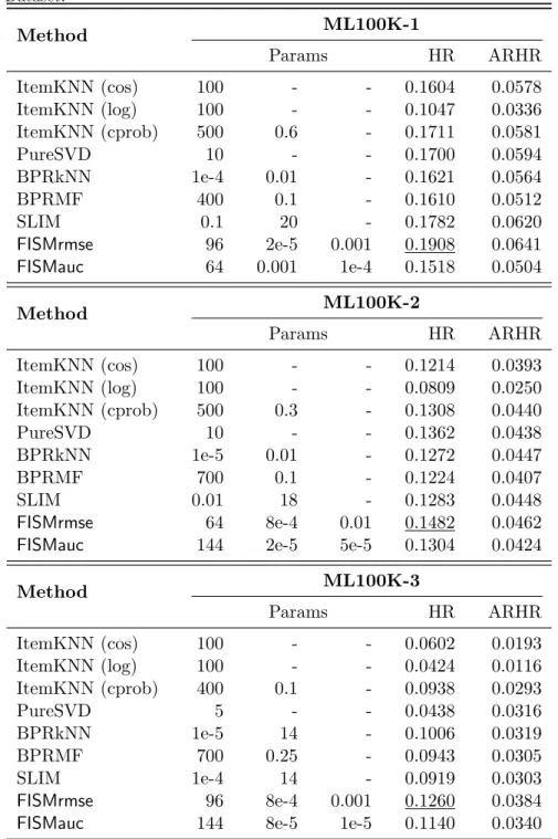
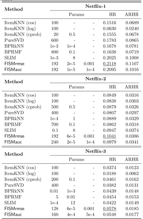
5.3.5 Comparison With Other Approaches . . . 38
5.4 Conclusion . . . 42
6 MPCF: Modeling Global and Local Preferences of Users in Collabora-tive Filtering 45 6.1 Introduction . . . 45
6.2 MPCF- Nonlinear Methods for CF . . . 48
6.2.1 MPCFi - Independent Features Model . . . 51
6.2.2 MPCFs- Shared Features Model . . . 52
6.2.3 Model Estimation . . . 52
6.3 Results . . . 56
6.3.1 Effect of Number of Local Preferences . . . 56
6.3.2 Effect of Bias . . . 56
6.3.3 Comparison with MaxMF . . . 58
6.3.4 Comparison with Other Approaches . . . 58
6.4 Conclusion . . . 63
7 ClustMF: Combined Neighborhood and Latent Factor Models for Top-N Recommender Systems 66 7.1 Introduction . . . 66
7.2 ClustMFMethod . . . 69
7.3 Results . . . 72
7.3.1 Effect of Number of Clusters . . . 72
7.3.2 Effect of Cluster Refinement . . . 73
7.3.3 Comparison With Other Approaches . . . 73
7.4 Conclusion . . . 74
8 Conclusion 76 8.1 Thesis Summary . . . 76
8.2 Future Research Directions . . . 78
References 80
List of Tables
2.1 Symbols used and definitions. . . 8 4.1 Datasets . . . 22 5.1 Performance of different bias schemes. . . 34 5.2 Comparison of performance oftop-Nrecommendation algorithms withFISMfor
ML100K Dataset. . . 39 5.3 Comparison of performance oftop-Nrecommendation algorithms withFISMfor
Netflix Dataset. . . 40 5.4 Comparison of performance oftop-Nrecommendation algorithms withFISMfor
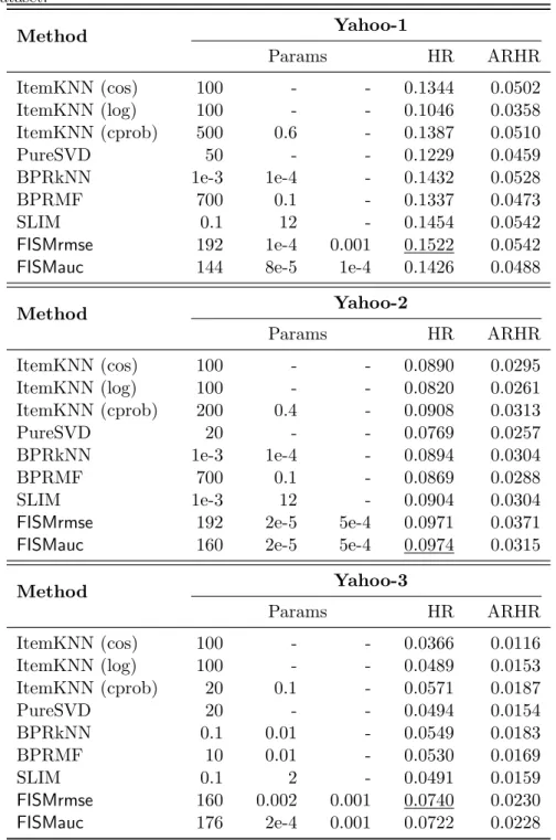
Yahoo Dataset. . . 41 6.1 Effect of Bias. . . 57 6.2 Comparison of performance of Rating Prediction algorithms withMPCF 60 6.3 Comparison of performance of Top-N recommendation algorithms with
MPCFfor Netflix Dataset . . . 62 6.4 Comparison of performance of Top-N recommendation algorithms with
MPCFfor Flixster Dataset . . . 63 7.1 Effect of Cluster Refinement (HR). . . 74 7.2 Comparison of performance of Top-N recommendation algorithms with
ClustMF . . . 75
List of Figures
5.1 Performance of induced Sparsity onS. . . 35
5.2 Effect of estimation approach on performance on ML100K dataset. . . . 35
5.3 Effect of estimation approach on performance on Netflix dataset. . . 36
5.4 Effect of estimation approach on performance on Yahoo dataset. . . 36
5.5 Non-negative and negative entries inS. . . 37
5.6 Performance for different values ofN for ML100K dataset. . . 42
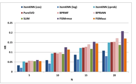
5.7 Performance for different values ofN for Yahoo dataset. . . 43
5.8 Effect of sparsity on performance for various datasets. . . 44
6.1 Modeling user preferences inMPCF. . . 49
6.2 Effect of Number of Local Preferences for Rating Prediction. . . 57
6.3 Effect of Number of Local Preferences for Top-N. . . 58
6.4 Comparison with MaxMF for Rating Prediction.. . . 59
6.5 Comparison with MaxMF for Top-N.. . . 61
6.6 Effect of Sparsity on top-N Performance.. . . 64
7.1 Effect of Number of Clusters on top-N Performance. . . 73
Chapter 1
Introduction
This thesis focuses on the development of new machine learning methods that arise primarily in the area of Recommender Systems. Recommender Systems are prevalent and are widely used in many applications. In particular, recommender systems have gained popularity via their usage in e-commerce applications to recommend items so as to help the users in identifying the items that best fit their personal tastes. Rec-ommender Systems helps the users to evaluate the potentially overwhelming number of options (termed as items) that a commercial service has to offer. Thus recommender systems have emerged as a key enabling technology for e-commerce. They perform the role of virtual experts who are keenly aware of users’ preferences and tastes, and corre-spondingly filter out vast amount of irrelevant data in order to identify and recommend the most relevant products. An example application is a video recommender system that helps users to select a movie to watch from a video catalogue. Popular online video streaming service like Netflix employs a video recommendation system to personalize the experience for each user. The recommendations are served based on the watch history of the user. Thus, the recommendations served for different users will be diverse.
Over the years, many algorithms have been developed for recommender systems. These algorithms make use of the user feedback (purchase, rating or review) to compute the recommendations. However, the state-of-the-art algorithms developed suffer from various issues like data sparsity, inability to effectively model users’ diverse interests, scalability, etc. The focus in this thesis is three fold. First, the focus is in dealing with the issue of data sparsity in building an efficient recommender systems. New
methods are developed to address the lack of feedback data for the users. Second, the focus is on modeling users’ multiple preferences. Users tend to have multiple and diverse preferences and the existing models are not sufficiently capable to capture these preferences. The problem of modeling users’ diverse interests is addressed in this thesis and a set of effective methods are presented. Third, the focus is on utilizing the benefits of both neighborhood models and latent factors model, which capture different and complementary characterisitics of the data. This is addressed by developing a new unified method which combines the benefits from both the models.
1.1
Key Contributions
There are two main problems associated with recommender systems. First, rating pre-diction problem, which aims to predict the rating for a user-item pair. Second, top-N recommendation problem, which aims to identify a short list of items that most fit a user’s personal preferences. In the recent years, top-N recommendation has gained popularity due to the increase of e-commerce services that serve various user needs. Rating prediction is still relevant in many application areas where the predicted rec-ommendation score is used. Thus, development of efficient top-N and rating prediction recommendation methods to generate high quality recommendations is highly desired.
1.1.1 Factored Item Similarity Methods (FISM)
In a real world scenario, the users provide feedback or purchase only a handful of items, from the possible set of thousands or millions of items. Thus the available user-item relational data is sparse. One class of existing state-of-the-art top-N methods provide recommendations by learning relations between items. However, they rely on co-purchase/co-rating information i.e., for the methods to learn meaningful relations and provide high quality recommendations, the training data must have enough users who have co-purchased many items. Thus, they suffer from data sparsity issue and fails to capture meaningful relations between users who do not have enough co-rated items. To effectively handle the real world sparse datasets, there is a need for methods which can effectively handle such sparse data.
In this thesis (Chapter 5), a new Factored Item Similarity Method (FISM) [1] for top-N recommendation is presented. There are multiple contributions from FISMmethods. First, it extends the factored item-based methods to the top-N problem, which allow them to effectively handle sparse datasets. Second it estimates the factored item-based top-N models using a structural equation modeling approach, and third it estimates the factored item-based top-N models using both squared error and a ranking loss.
1.1.2 Modeling Global and Local Preferences of Users in Collaborative Filtering (MPCF)
Many existing state-of-the-art rating prediction and top-N collaborative filtering meth-ods model user preferences as a vector in a latent space. These methmeth-ods assume that the user preference is consistent across all the items that the user has rated and thus model the user using a single user preference vector. However, user preferences are typ-ically much more complicated than that. Many users can have multiple tastes and their preferences can vary with each such taste. To address this, a recently proposed method extended the latent representation models to include multiple preference vectors for each user, in order to capture the user’s preferences for each of the preferences separately. In this thesis (Chapter 6), we propose a different user modeling approach (MPCF)[2] that models the user’s preference as a combination of global preference and local preferences components. Using this user modeling approach, we propose two different methods based on the manner in which the global preference and local preferences components interact. In the first approach, the global component models the user’s strong prefer-ences on a subset of item features, while the local preferprefer-ences component models the tradeoffs the users are willing to take on the rest of the item features. In the second approach, the global preference component models the user’s overall preferences on all the item features and the local preferences component models the different tradeoffs the users have on all the item features, thereby helping to fine tune the global preferences. An additional advantage of MPCF is that, the user’s global preferences are estimated by taking into account all the observations, thus it can handle sparse data effectively. A comprehensive set of experiments on multiple datasets show that the proposed model outperforms other state-of-the-art recommendation methods for both rating prediction and top-N recommendation tasks.
1.1.3 Cluster Based Matrix Factorization Methods
Neighborhood models like UserKNN and ItemKNN are intuitive and simple to imple-ment. They are most effective at detecting localized relationships and thus helps to better explain the recommendations provided to the user. The recommendations pro-vided by neighborhood methods are backed by the observed data (in terms of co-rated users/items), and thus are somewhat ”familiar” to the user, as they can be shown to be explicitly related to an item they have consumed in the past. However, the main limita-tion of neighborhood models is that the top recommended similar items are computed using only a small fraction of the user’s preferences. Thus, they fail to capture the sum total of the weak signals provided by all of the user’s preferences. On the other hand, latent factor models utilize all the user’s preferences in learning the user and item latent factors to produce the recommendations. Thus, they are generally effective in capturing the overall relations that exist among the users and the items. Although individually, latent factor models have been shown to produce superior top-N recommendations com-pared to neighborhood models, the recommendations provided by latent factor models cannot be easily explained to the user; the notion of observed item neighborhood is not present and thus the user familiarity is absent. For top-N recommendation task, the absence of familiarity might affect the choice a user makes from the computed list of top-N recommended items, since there is a potential for the user to lose the context on why a particular item was recommended to him/her, in particular for items which lie “far away” in the neighborhood of the items rated by the user. Hence, there is a need for a combined model, which can capitalize on both the benefits of the neighborhood models and the latent factor models. That is, a model which can capture the localized relationships like neighborhood models to bring in the familiarity aspect to the users and also capture the global relations between users and items like the latent factor models to provide better recommendations. In this thesis (Chapter 7), we propose a new method calledClustMFwhich is designed to combine the benefits of both the neighborhood and latent factor models. The benefits of latent factors models are utilized by modeling the users and items similar to the standard MF based methods. That is, the users and items are represented with latent vectors, where the item latent vectors correspond to the latent features associated with them and the user latent vectors correspond to the user preferences on the item features. The benefit of neighborhood models are brought
into the model, by introducing biases at the cluster level. These cluster level biases are introduced to capture the localized relationships present in the user and/or item neighborhoods. For an item to be part of the top-N list of the user, along with the latent factors component producing a high score, the corresponding user cluster bias and item cluster bias must also be high. That is, to have a high user cluster bias, the item must be in the neighborhood of the items that the user has liked in the past and to have a high item cluster bias, the user must be in the neighborhood of the users who have liked the item. A comprehensive set of experiments show that the proposed model outperforms the rest of the state-of-the-art methods for top-N recommendation task.
1.2
Outline
This thesis is organized as follows:
• Chapter 2 provides definitions and notation which is used throughout this thesis.
• Chapter 3 provides details of the existing research related to the different problems and methodologies presented in this thesis.
• Chapter 4 presents the evaluation methodology employed, the different datasets used and the different state-of-the art algorithms that we compare the performance for various methods presented in this thesis.
• Chapter 5 presents a new Factored Item Similarities Method (FISM) for top-N recommendation problem is presented.
• Chapter 6 presents a new set of Non Linear Factorization (MPCF) methods which better models the users’ multiple interest preferences.
• Chapter 7 presents a new Combined Neighborhood and Latent Factors Models (ClustMF) for top-N recommender system is presented.
• Chapter 8 summarizes the conclusions of the research presented in this thesis and some future research directions.
1.3
Related Publications
The work presented in this thesis and the related work has been published in leading conferences and journals in data mining and knowledge discovery. The related publica-tions are listed as follows:
• Santosh Kabbur, Eui-Hong Han and George Karypis. Content-based methods for predicting web-site demographic attributes. In Proceedings of the 10th IEEE ICDM International Conference on Data Mining 2010, pages 863–868, 2010. • Santosh Kabbur, Huong Le, Luciano Pollastrini, Ziran Sun, Keri Mills, Kevin
Johnson, George Karypis, Wei-Shou Hu. Multivariate analysis of cell culture bio-process datalactate consumption as bio-process indicator. InJournal of biotechnology, 2012.
• Santosh Kabbur, Xia Ning and George Karypis. FISM: factored item similarity models for top-N recommender systems. InProceedings of the 19th ACM SIGKDD international conference on Knowledge discovery and data mining, pages 659–667, 2013.
• Santosh Kabburand George Karypis. NLMF: Non-Linear Matrix Factorization Methods for Top-N Recommender Systems. In Proceedings of IEEE Workshop on Domain Driven Data Mining, ICDMW, 2014.
• Santosh Kabburand George Karypis. MPCF: Modeling Global and Local Pref-erences of Users in Collaborative Filtering InProceedings of the 38th Annual ACM Special Interest Group On Information Retrieval, SIGIR, 2015 (under review). • Santosh Kabbur and George Karypis. ClustMF: Combined Neighborhood and
Chapter 2
Definitions and Notations
All vectors are represented by bold lower case letters and they are row vectors (e.g., p,q). All matrices are represented by bold upper case letters (e.g.,R,W). Theith row of a matrix A is represented by ai. We use calligraphic letters to denote sets (e.g., C, D). A predicted value is denoted by having a˜(tilde) over it (e.g., ˜r) and an estimated value is denoted by having aˆ(hat) over it (e.g., ˆr).
CandDare used to denote the sets of users and items, respectively, whose respective cardinalities arenandm(i.e.,|C|=nand|D|=m). MatrixRwill be used to represent the user-item feedback/rating matrix of size n×m, i.e.,R∈Rn×m. Symbols u and i
are used to denote individual users and items, respectively. An entry (u, i) inR, denoted by rui, is used to represent the rating on item i by user u. For implicit feedback, Ris
converted to a binary matrix. If the user has provided feedback for a particular item, then the corresponding entry inR is 1, otherwise it is 0. We will refer to the entries for which the user has provided feedback as rated items and those for which the user has not provided feedback as unrated items.
For quick reference, all the important symbols used, along with their definition is summarized in Table 2.1.
Table 2.1: Symbols used and definitions. Symbol Definition
C Set of users. D Set of items.
u,i Individual useru, itemi.
n,m Number of users and items,n=|C|, m=|D|.
k Number of latent factors.
l Number of latent factors for local preferences component inMPCFi.
T Number of user local preferences.
lu,li Number of user and item clusters.
ci Item cluster assignment cu User cluster assignment
R User-Item Feedback/Rating Matrix,R∈Rn×m. R+
u Set of items for which useru has provided feedback
R−u Set of items for which useru has not provided feedback
rui Rating by useru on itemi.
ˆ
rui Predicted rating for useru on itemi.
bu User Bias vector,bu∈R1×n.
bi Item Bias vector,bi∈R1×m.
Bu User-Interest Bias matrix,Bu∈Rn×T.
BU User Cluster Bias matrix,BU∈Rn×li. BI Item Cluster Bias matrix,Bu∈Rm×lu.
P User Latent Factor Matrix,P∈Rn×k. W User Latent Factor Tensor,W∈Rn×k×T. Q Item Latent Factor Matrix,Q∈Rm×k.
Y Item Latent Factor Matrix, for local preferences component in MPCFi,Y∈Rm×l.
S Item-Item Similarity matrix,S∈Rm×m
λ `F regularization weight.
ρ Sampling factor for learning algorithm. η Learning Rate for learning algorithm.
n+u Number of items for which useru has provided feedback
λ,γ `F regularization weights
Chapter 3
Background and Related Work
Over the years, many algorithms and methods have been developed to address the rating prediction and top-N recommendation problem [3, 4, 5, 6, 7] in recommender systems. These algorithms make use of the user feedback data available in the form of purchase, rating or review. Typically these algorithms represent the feedback information as a user-purchase matrix and act on it. The existing methods can be broadly classified into two groups: collaborative filtering (CF) [8] based methods and content based methods. User/Item co-rating is used in collaborative filtering methods to build models. One class of CF methods, referred to as nearest-neighborhood-based methods, compute the similarities between the users/items using the co-rating information and new items are recommended based on these similarity values. Another class of CF methods, referred to as model-based methods, employ a machine learning algorithm to build a model (in terms of similarities or latent factors), which is then used to perform the recommenda-tion task. These methods learn representarecommenda-tion for users and items in common latent space and the recommendation score for a given user and item pair is computed as the dot product of the corresponding user and item latent vectors. In content based methods, users/items features are used to build models [9, 10]. In this thesis work, the focus is limited only to CF based methods. In the next section we discuss some of the state-of-the-art CF methods in detail.
3.1
Existing Methods
User (UserKNN) and Item (ItemKNN)k-nearest neighbors UserKNN [11, 12] is a classical user based CF method, which computesk-nearest neighbors for each user, based on their rating profiles. These nearest neighbors are then used to predict the rating for a user on an unrated item as the weighted average of the rating of the nearest neighbors of the user.
Similar to UserKNN method, ItemKNN [13, 14, 15] is a CF based method which identifies the k-nearest neighbors in the items space, based on their co-rating informa-tion. These item neighbors are then used to recommend new items to the users, based on the items which are similar to the items rated by the user.
The user/item nearest neighbors are calculated from user-item rating matrix in a collaborative way using a vector similarity measure like cosine similarity, pearson cor-relation etc., These methods are simple and easier to implement and are nonlinear in terms of the preferences of the user, which are implicitly captured via the nearest neigh-bors. However, they rely on the co-rating information between the users to compute the similarity. Thus, it suffers from data sparsity issue and fails to capture relations between users who do not have enough co-rated items.
Matrix Factorization (MF) Methods In recent years, approaches based on matrix factorization of the user-item rating matrix have emerged as a very powerful technique for rating prediction and top-N recommendation tasks [16, 17, 18, 19, 3, 20, 21, 22, 23]. MF based methods are known to outperform [24] other models including Bayesian models URP [25] and PLSA [26]. In these methods, the rating matrixRis approximated as a product of two low-rank matrices P and Q, where P ∈Rn×k is the users latent vector matrix, Q∈ Rm×k is the items latent vector matrix, k is the number of latent factors andkn, m. The recommendation score of a userufor itemiis then predicted as,
ˆ
rui=puqTi, (3.1)
wherepuis the latent vector associated with useruandqi is the latent vector associated
In [27, 28], classical dimensionality reduction technique, Singular Value Decompo-sition (SVD) is applied on the rating matrix R. The resulting factorized matrices are used to represent the users and items latent factors. While applying the SVD algorithm, they impute the missing values of R with zeros. Thus, the user item rating matrixR is estimated by the factorization:
ˆ
R=U·Σ·V, (3.2)
where, U is a n ×k orthonormal matrix, V is a k ×m matrix and Σ is a k×k
diagonal matrix containing the first ksingular values. The product U·Σ can be used to represent the user factors and V the item factors. The predicted recommendation score can then be computed similar to the MF method. Most of the MF based methods employ either Alternating Least Squares (ALS) [21] or Stochastic Gradient Descent (SGD) [29] based methods to learn the low dimensional embeddings of the users and items. One potential limitation of these approaches is that, although the user and item latent factors are learnt in a collaborative fashion, unlike neighborhood methods it learns the user and item latent factors by incorporating all the ratings in the data, and thus it does not explicitly take the neighborhood of the user/item into account while making the predictions.
Many extensions and variations to MF based methods are also proposed in the recent years. A probabilistic based approach for matrix factorization is proposed in [30]. Temporal dynamics is incorporated into matrix factorization in [31] to better model the users’ time sensitive preferences. Blending of various CF models was proposed in [32, 33] to achieve the best rating prediction performance for the Netflix Prize [34]. In [6, 7], a Weighted Regularized Matrix Factorization (WRMF) method is proposed. This method is formulated as a regularized Least-Squares (LS) problem, in which a weighting matrix is used to differentiate the contributions from observed purchase/rating activities and unobserved ones. A Max-Margin Matrix Factorization (MMMF) method is proposed [24, 35, 36], which requires a low-norm factorization of the user-item matrix and allows unbounded dimensionality for the latent space. This is implemented by minimizing the tracenorm of the reconstructed user-item matrix from the factors. Sindhwani et al [37] proposed a Weighted Non-Negative Matrix Factorization (WNNMF) method, in which they enforce nonnegativity on the user and item factors so as to lend part-based
interpretability to the model. Probabilistic Latent Semantic Analysis (PLSA) technique was applied for collaborative filtering by Hofmann in [26]. It was also shown to be equivalent to non-negative matrix factorization (NNMF). Sparse matrix factorization algorithms are used in [38, 39, 40] to reduce the computational complexity in the context of rating prediction problem. In [41], Yu et. al. formulate the collaborative filtering as a maximum-margin matrix approximation problem with regularization. Agarwal et. al. in [42], proposed a regression based latent factor model for rating prediction problem.
NSVD & SVD++ One other popular extension of MF based methods is called NSVD and was developed by Paterek in [43]. This is a factored item-item collaborative filtering method developed for the rating prediction problem. In this method, an item-item similarity was learned as a product of two low-rank matrices, P and Q, where P∈Rm×k,Q∈Rm×k, andkm. This approach extends the traditional item-based neighborhood methods by learning the similarity between items as a product of their corresponding latent factors. Given two items iand j, the similaritysim(i, j) between them is computed as the dot product between the corresponding factors from PandQ i.e., sim(i, j) = pi·qTj. The rating for a given user u on item j is both predicted and
estimated as, ˆ rui= ˜rui=bu+bi+ X j∈R+u pjqTi , (3.3)
wherebu andbi are the user and item biases andR+u is the set of items rated byu. The
parameters of this model are estimated as the minimizer to the following optimization problem: minimize P,Q 1 2 X u∈C X j∈R+u krui−ˆruik2F + β 2(kPk 2 F +kQk2F), (3.4)
where ˆrui is the estimated value for useru and itemj (as in Equation 3.3).
In another set of methods [44, 21], the latent factor models and neighborhood based methods are combined. In a popular based on NSVD, Koren proposed a hybrid approach called SVD++ [5]. This method smoothly merges the latent factor and neighborhood based models. The proposed model is extended to include both implicit [45] and explicit user feedback data. The latent factors part of the model consists of the standard user and item latent factors along with the second set of item factors which are used to model the
asymmetric relations between the items in the latent space. For the neighborhood part of the model, the relations between the items are explicitly learned in the form of weights between the items. The proposed model was shown to outperform rest of the state-of-the-art methods. One of the limitations of this method is w.r.t. learning large number of parameters. Along with modeling each user with a latent vector and each item with two latent vectors, it also learns a weight vector for each item to learn the item similarities in the neighborhood component. To reduce the number of parameters learned in the neighborhood component, only top-k nearest neighbors based on the items corating information is used to learn the item relations. Even then, hundereds to thousands of additional parameters needs to be learned for each of the items. Learning these parameters is computationally expensive and large number of parameters can potentially lead to an overfitted model. Also, both these models (i.e., NSVD and SVD++) were evaluated by computing the root mean square error (RMSE) on the test ratings in the Netflix competition data set. Hence the goal of these models was to minimize the RMSE and only the non-zero entries of the rating matrix were used in training.
Sparse Linear Methods (SLIM) Recently, a novel top-N recommendation method has been developed, called SLIM [46], which improves upon the traditional item-based nearest neighbor collaborative filtering approaches by learning the item relationships from the data, a sparse matrix of aggregation coefficients that are analogous to the traditional item-item similarities. SLIM predicts the recommendation scores of a user
u for all items as,
˜
ru =ruS, (3.5)
where ru is the rating vector of u on all items and S is a m×m sparse matrix of
aggregation coefficients.
MatrixS can be considered as an item-item similarity matrix, and as such the rec-ommendation strategy employed by SLIM is similar in nature to that of the traditional item-based nearest-neighbor top-N recommendation approaches [14]. However, unlike these methods, SLIM directly estimates the similarity values from the data using a si-multaneous regression approach, which is similar to structural equation modeling with no exogenous variables [47]. Specifically, SLIM estimates the sparse matrix S as the
minimizer for the following regularized optimization problem: minimize S 1 2kR−RSk 2 F + β 2kSk 2 F +λkSk1 (3.6) subject to S≥0, diag(S) = 0,
wherekSkF is the matrix Frobenius norm ofS andkSk1 is the entry-wise`1-norm ofS. In Equation 3.6, RS is the estimated matrix of recommendation scores (i.e., ˜R). The constraint diag(S) = 0 conforming to the structural equation modeling is also applied to ensure that rui is not used to compute rui. The non-negativity constraint is applied
on S so that the learned S corresponds to positive aggregations over items. In order to learn a sparse S, SLIM introduces the `1-norm of S as a regularizer in Equation 3.6 [48]. Along with `1-norm, `F-norm is also used as another regularizer, which leads the
optimization problem to an elastic net problem [49]. The `F-norm is used to prevent
overfitting of the model to the training data. The matrix Slearned by SLIM is referred to as SLIM’s aggregation coefficient matrix. Extensive experiments in [46] have shown that SLIM outperforms the rest of the state-of-the-art top-N recommendation methods. SLIM has been shown to achieve good performance on a wide variety of datasets and to outperform other state-of-the-art approaches. However, an inherent limitation of SLIM is that it can only model relations between items that have been co-purchased/co-rated by at least some users. As a result, it cannot capture transitive relations be-tween items that are essential for good performance of item-based approaches in sparse datasets.
Nonlinear latent factorization (MaxMF) One of the recently developed methods for top-N recommendation called MaxMF [50], extends the matrix factorization based approaches by representing the user with multiple latent vectors, each corresponding to a different “taste” associated with the user. These different tastes associated with each user representation are termed as interests. The assumption behind this approach is that, by letting the users to have multiple interests, it helps to capture user preferences better, especially when the itemsets or user’s interests are diverse. Thus, the user is represented with T different interests and a max function based nonlinear model was proposed. The model takes the maximum scoring interest as the final recommendation score for a given user item pair, i.e., the interest which matches the best with the given
item is captured in this model. In other words, the set of items is partitioned into T
partitions for each user, and this partitioning process is personalized on the user. For each such item partition a different scoring function is used to estimate the rating. The user factors are thus represented by a tensorP, whereP∈Rn×k×T. The items factors, Q remains similar to MF based approaches. Thus, each user u is represented by pu,
where pu ∈Rk×T. For a given user u and item i pair, the predicted recommendation
score is calculated by computing T dot products between each of the T user vectors and the corresponding item vector. The highest scoring dot product is taken as the estimated/predicted rating. That is,
ˆ
rui= max t=1,...,Tputq
T
i, (3.7)
where the max function computes the maximum of the set of dot products between each of put andqi.
It was shown that MaxMF achieves better top-N recommendation performance com-pared to other state-of-the-art methods. However, a limitation of this method is that it assumes that the interest-specific preferences of the users are completely different. Another limitation of MaxMF is w.r.t. data sparsity. When the data gets sparse i.e., when less preference data is available for each user, this approach can potentially dilute the learnt latent factors for users who do not have enough diversity in their itemsets due to lack of support (in terms of number of rated items) for each of the interests. This problem is magnified, as the data gets sparser.
In [51], a nonlinear matrix factorization approach with Gaussian processes is pro-posed. This method uses a kernelized form for the model. Salakhutdinov et. al. in [52] applied Restricted Boltzmann machines for collaborative filtering, which is a form of neural networks that introduces nonlinearities via Gaussian hidden units.
Bayesian Personalized Ranking (BPR) Methods In one of the recent methods, Top-N recommendation has also been formulated as a ranking problem. Rendle et al [53] proposed a Bayesian Personalized Ranking (BPR) criterion, which is the maximum posterior estimator from a Bayesian analysis and measures the difference between the rankings of items which are purchased and not purchased by the user. A differentiable loss function is used to optimize the AUC. BPR was adopted for both item knn method (BPRkNN) and MF methods (BPRMF) as a general objective function.
Clustering Based Methods In another class of methods, clustering is employed to improve the scalability and accuracy of the CF methods. In [54, 55, 56, 57, 58], clustering techniques are used to partition the users or items into clusters and a memory-based collaborative algorithm like UserKNN or ItemKNN is applied to make predictions for each of the cluster. Ungar et. al. [59] use variations of k-means and Gibbs sampling to cluster users based on the items they rated and clustering items based on the users who rated them. Users are then reclustered based on the number of items they rated and similarly the items are reclustered based on the number of users who ratem them. This alternating process is repeated till convergence. In [60], flexible mixture model is applied to cluster both the users and item at the same time, allowing the users and items to be part of multiple clusters. A membership score is assigned to each of the clusters that the users and items belong to. Many other clustering based approaches have been proposed to improve the scalability of the existing CF approaches [61, 62, 63, 64]. A good survey on the clustering based CF methods can be found in [65].
Other methods Several other methods has been proposed in the recent years that formulate the top-N problem as a ranking problem. For a given user, pairwise opti-mization methods [66] like Ordinal Regression [67], WSABIE [68], COFI-RANK [69], EigenRank [70] and CLiMF [71] optimize a ranking loss with the goal of ranking higher valued items above lower scoring items. Many of these methods rely on Learning to Rank optimization algorithms used in information retrieval domain [72]. A different approach was proposed in [73], in which the rating prediction problem was formulated as a binary classification problem and a one-class classifier was built for each user, and all the classifiers were learned and boosted together.
A review on early works of traditional collaborative filtering is available in [19] and a review on recent collaborative filtering methods can be found in [3, 65]. Matrix Factor-ization has gained popularity in the recent years and has also achieved the state-of-the-art recommendation performance pstate-of-the-articularly on large-scale rating prediction problems. A review on such MF based methods for recommender systems is available in [16]. In re-cent years, many methods and frameworks [74, 75, 76, 77, 78, 79] have been proposed to improve the scalability of the collaborative filtering algorithms to large-scale problems.
3.2
Loss Functions
In this thesis, we employ two different loss functions to estimate the parameters of the proposed models. First, is the squared loss, which computes the total loss as the sum of the square of the difference between the actual value and the estimated value. Given a set of data points X, the squared error loss function is given by,
L(·) = X
x∈X
(x−xˆ)2, (3.8)
where x is the actual value and ˆx is the estimated value of the data.
Second loss function used is the BPR criterion function. BPR employs a pairwise ranking criterion between the data points. Unlike squared loss which computes loss on the ground truth value of the data point, BPR computes loss only the estimated values of the data points. It measures the difference between the estimated values of the data points which have a higher value with the ones which have a lower value. Given a set of data pointsX, the BPR criterion is given by,
L(·) = X (xi,xj)∈X
lnσ(ˆxi−xˆj) (3.9)
where xi is a higher valued data point compared to xj, σ(x) is the sigmoid function,
i.e., σ(x) = 1/(1 +e−x). The sigmoid and log functions are used to make the criterion function differentiable, which is helpful in using gradient based methods to optimize the objective function corresponding to the ranking criterion.
3.3
Optimization Algorithms
In this thesis we utilize the Stochastic Gradient Descent (SGD) based algorithm to opti-mize (miniopti-mize/maxiopti-mize) the objective function associated with the different proposed methods. First the general formulation of the SGD algorithm is presented. Then the SGD algorihm in the context of squared loss and BPR criterion is presented.
Stochastic Gradient Descent (SGD) is a gradient descent optimization method for minimizing an objective function that is expressed as a sum of differentiable func-tions. SGD based approximations are known to perform poorly for optimization tasks, while their performance is extermely good for machine learning tasks [29]. Historically,
Stochastic gradient algorithms have been associated with back-propagation learning methods in multilayer neural networks, which can be very challenging non-convex prob-lems.
Given a objective function Q(w), which is a sum of differentiable functions, i.e.,
Q(w) = Pn
i=1Qi(w), where Qi(w) is the function associated with i-th sample in the data set andnis the number of data samples, a standard gradient descent (also known as Steepest Gradient Descent) based iterative optimization technique updates the weights
w on of the basis of the gradients∇Qi(w) in each iteration. That is,
wt=wt−1−η
n
X
i=1
∇Qi(w), (3.10)
where η is the learning rate and tis the current iteration number.
The SGD is a simplification of the steepest gradient descent. Instead of computing the gradient of Qi(w) exactly, each iteration estimates this gradient on the basis of a
single randomly selected data sample. That is, given a sample i, the SGD update rule is given by,
wt=wt−1−η∇Qi(w). (3.11)
This update is repeated for each of the randomly picked training sample of the data set. Several passes over the training data is made until the algorithm converges. The generalized pseudocode for the SGD algorithm is given in Algorithm 1.
SGD is shown to converge to a local minimum and have a convergance rate which is independent of the size of the data. Thus SGD is highly suitable for large scale datasets. Another advantage of SGD is that, since the SGD algorithm does not need to remember which examples were visited during the previous iterations, it can process data samples on the fly in an online setting.
Squared Loss
In case of squared loss, the parameters of the model, Θ are learned by minimizing the following regularized objective function,
Squared−OP T = X
x∈X
(x−xˆ)2+λΘkΘk2 (3.12) where λΘ is the regularization constant corresponding to parameter Θ. The details of the corresponding SGD based learning algorithm is provided in Algorithm 2.
Algorithm 1 SGD:Opt.
1: procedure SGD Opt
2: w← weight vector to learn
3: η← learning rate
4: iter←0
5: Initw with random values
6:
7: whileiter < maxIter or error on validation set decreasesdo
8: for all i= 1,2,3, . . . , n do 9: wt←wt−1−η∇Qi(w) 10: end for 11: iter←iter+ 1 12: end while 13: 14: return w 15: end procedure
Bayesian Personalised Ranking (BPR)
Bayesian Personalised Ranking (BPR) [53] is a generic method for solving the person-alized ranking task. The approach mainly consists of a general optimization criterion (known as BP R−OP T) for personalized ranking. BPR measures the difference be-tween the rankings of items which are purchased and not purchased by the user. For a given useru, purchased itemiand unpurchased itemj, ˆxuij(Θ) represents an arbitrary
real valued function which approximates the bayesian formulation of the personalized ranking, where Θ captures the relationship between the triplet (u,i,j). The generic framework of BPR lets the underlying method like matrix factorization or k-nearest neighbors to model these relationships between the users and items. A differentiable loss function is used to optimize the criterion which is shown to optimize the AUC metrix. Given DS, a set of sampled triplets of (u, i, j), the objective function of the
BPR is given by,
BP R−OP T = X (u,i,j)∈DS
lnσ(ˆxuij)−λΘkΘk2 (3.13)
whereλθ are model specific regularization parameters. Parameters of theBP R−OP T
can be learnt using a Stochastic Gradient Descent (SGD) based method. The algorithm for learning the model parameters using a SGD based method is outlined in Algorithm 3.
Algorithm 2 SquaredLoss:Opt.
1: procedure SquaredLoss Opt 2: w← parameter vector to learn
3: η← learning rate
4: iter←0
5: Initw with random values
6:
7: whileiter < maxIter or error on validation set decreasesdo
8: for all xi ∈X do 9: ei =xi−xˆi 10: wt←wt−1+η·(ei−λΘ·Θ) 11: end for 12: iter←iter+ 1 13: end while 14: 15: return w 16: end procedure Algorithm 3 BPR:Opt. 1: procedure BPR OPT
2: DS ← sampled triplets (u, i, j) fromR 3: η← learning rate
4: Θ← parameters to learn
5: Init Θ with random values
6:
7: whilenot convergeddo
8: draw (u, i, j) from DS randomly 9: Θ←Θ +η( e−xuijˆ 1+e−xuijˆ · ∂ ∂Θxˆuij+λΘ·Θ) 10: end while 11: 12: return Θ 13: end procedure
Chapter 4
Datasets & Evaluation
Methodology
4.1
Datasets
In this thesis, the performance of proposed methods is evaluated on different real datasets, namely ML100K, ML1M, Netflix, Grades, Flixster and Yahoo Music. ML100K and ML1M are the subsets of data obtained from the MovieLens1 research project, Netflix is a subset of data extracted from Netflix Prize dataset2 , Grades is the dataset collected from a student database at an academic institution and it consists of students as users and courses as items and the grades obtained by the students in courses rep-resents the rating values, Flixster is a subset of data extracted from publicly available data set collected from Flixster and finally Yahoo Music is the subset of data obtained from Yahoo! Research Alliance Webscope program3 . For each of the ML100K, Netflix, Yahoo and Flixster datasets, different versions at different sparsity levels are created. This was done to specifically evaluate the performance of the proposed method on sparse datasets. For each dataset, a random subset of users and items are selected from the main dataset. These datasets are represented with a’-1’ suffix. Keeping the same set of users and items, the first sparser version of the datasets with the ’-2’ suffix are created
1 http://www.grouplens.org/node/12 2
http://www.netflixprize.com/
3 http://research.yahoo.com/academic relations
by randomly removing entries from the first datasets’ user-item matrices. The second sparser version of the datasets with the ’-3’ suffix are similarly created by randomly removing entries from second datasets’ user-item matrices. Note that all these datasets have rating values and we converted them into implicit feedback by setting the positive entries to 1 to evaluate the proposed methods in the context of the top-N recommen-dation task. The characteristics of all the datasets is summarized in Table 4.1. For the different methods presented in this thesis, we use a subset of the listed datasets.
Table 4.1: Datasets
Dataset #Users #Items #Ratings Density ML100K 943 1,349 99,287 7.80% ML100K-1 943 1,178 59,763 5.43% ML100K-2 943 1,178 39,763 3.61% ML100K-3 943 1,178 19,763 1.80% ML1M 6,040 3,952 1,000,209 4.19% Netflix 5,403 2,933 2,197,096 13.86% Netflix-1 6,079 5,641 429,339 1.25% Netflix-2 6,079 5,641 221,304 0.65% Netflix-3 6,079 5,641 110,000 0.32% Netflix-4 5,403 2,933 1,649,174 10.41% Grades 19,319 9,562 422,203 0.23% Flixster-1 4,627 3,295 1,184,817 7.77% Flixster-2 4,627 3,295 889,842 5.84% Yahoo 5,824 15,869 1,440,212 1.56% Yahoo-1 7,558 3,951 282,075 0.94% Yahoo-2 7,558 3,951 149,050 0.50% Yahoo-3 7,558 3,951 75,000 0.25% The “#Users”, “#Items” and “#Ratings” columns are the number of users, items and ratings respectively, in each of the datasets. The ”Rat-ing Scale” column is the range of the rat”Rat-ings present. The “Density” col-umn is the density of each dataset (i.e., density = #Ratings/(#Users× #Items)).
4.2
Evaluation Methodology
The performance of the methods presented in this thesis are evaluated using a 5-fold Leave-One-Out-Cross-Validation (LOOCV) method similar to the one employed in [46]. Training and test set is created by randomly selecting one rated item per user from the dataset and placing it in the test set. The rest of the data is used as the training set. This process is repeated to create five different folds. Only for the Grades dataset, the test set is created by using the grades of the last semester for each student. The rest of the grades from previous semesters is used as the training set. The training set is used to build the model and the trained model is then evaluated on the test set. For rating prediction task, the recommendation scores from the trained model is used as the predicted ratings. For the top-N recommendation task, the trained model is then used to generate a ranked list of size-N items for each user. The model is then evaluated by comparing the ranked list of recommended items with the item in the test set. Unless specified, for all the results presented in this thesis,N is equal to 10.
4.3
Performance Metrics
The recommendation quality of the rating prediction task, for each user the trained model is used to predict the rating for the unrated items in the test set. The model is then evaluated by computing the test metric for each of the test user-item rating pair. The rating prediction quality is measured using Root Mean Square Error(RMSE). RMSE is defined as,
RM SE = 1 |T est| s X rui∈T est (rui−rˆui)2,
whererui is the ground truth value and ˆruiis the predicted rating value for a given user
u and itemiand T est is the test data consisting of test user-item pairs.
For the top-N recommendation task, the trained model is evaluated by comparing the ranked list of recommended items with the item in the test set. The recommendation quality for top-N recommendation task is measured using Hit Rate (HR) and Average Reciprocal Hit Rank (ARHR) [14]. HR is defined as,
HR= #hits #users,
where #hits is the number of users for which the model was successfully able to recall the test item in the size-N recommendation list and #usersis the total number of test users. The ARHR is defined as,
ARHR= 1 #users #hits X i=1 1 posi ,
where posi is the position of the test item in the ranked recommendation list for the
ith hit. ARHR represents the weighted version of HR, as it measures the inverse of the position of the recommended item in the ranked list.
We chose RMSE, HR and ARHR as evaluation metrics since they directly measure the performance of the model on the ground truth data i.e., what users have already provided feedback for.
4.4
Comparison Algorithms
The performance of the different methods proposed in this thesis are compared against to that achieved by a number of the current state-of-the-art methods. These meth-ods include UserKNN [11], ItemKNN [14], ItemKNN (cprob) [14], ItemKNN (log)4 , PureSVD [28], MF [28], MaxMF [50], BPRMF & BPRkNN [53] and SLIM [46]. The details of these methods are provided in the Section 3.1. This set of methods consti-tute the current state-of-the-art for rating prediction and top-N recommendation task. Hence they form a good set of methods to compare and evaluate our proposed approach against.
The following parameter space was explored for each of these methods and the best performing model in that parameter space in terms of RMSE/HR is reported. For UserKNN, PureSVD, MF, BPRMF and MaxMF, parameter k was selected from the range 2 to 800. For ItemKNN (cprob), the α parameter was selected from the range 0 to 1. Learning rate and regularization constants for MF and BPRMF was selected from the range 10−5 to 1.0. For BPRkNN, the learning rate andλ were selected from the range 10−5 to 1.0 For SLIM and MaxMF, the regularization constants were selected from the range 10−5 to 20. For MaxMF the number of local preferencesT was selected from the range 1 to 6.
Chapter 5
FISM
: Factored Item Similarity
Methods for Top-N
Recommender Systems
This chapter focuses on developing an effective algorithm for top-N recommender sys-tems. A novel Factored Item Similarities based methodFISM is proposed, which learns the item-item similarity matrix as a product of two low-dimensional latent factor ma-trices. This factored representation of the item-item similarity matrix allows FISM to capture and model relations between items even on very sparse datasets. Our exper-imental evaluation on multiple datasets and at different sparsity levels confirms that and shows that FISM performs better than SLIM and other state-of-the-art methods. Moreover, the relative performance gains increase with the sparsity of the datasets.
5.1
Introduction
In real world scenarios, users typically provide feedback (purchase, rating or review) to only a handful of items out of possibly thousands or millions of items. This results in the user-item rating matrix becoming very sparse. Methods like SLIM (as well as traditional methods like ItemKNN), which rely on learning similarities between items, fail to capture the dependencies between items that have not been co-rated by at least
one user. It can be shown that the minimizer in SLIM will have sij = 0, if i and j
have not been co-rated by at least one user. But two such items can be similar to each other by virtue of another item which is similar to both of them (transitive relation). Methods based on matrix factorization, alleviate this problem by projecting the data onto a low dimensional space, thereby implicitly learning better relationships between the users and items (including items which are not co-rated). However, such methods are consistently out-performed by SLIM.
To overcome this problem, the proposed item-orientedFISMmethod uses a factored item similarity model similar in spirit to that used by NSVD and SVD++. Learning the similarity matrix by projecting the values in a latent space of much smaller dimen-sionality, implicitly helps to learn transitive relations between items. Hence, this model is expected to perform better even on sparse data, as it can learn relationships between items which are not co-rated.
ComparingFISMwith NSVD, besides the fact that these two methods are designed to solve different problems (top-N vs rating prediction), their key difference lies in how the factored matrices are estimated. FISM employs a regression approach based on structural equation modeling in which, unlike NSVD (and SVD++), the known rating information for a particular user-item pair (rui) is not used when the rating for that item
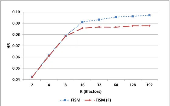
is being estimated. This impacts how the diagonal entries of the item-item similarity matrix corresponding to S = PQT influence the estimation of the recommendation score. Diagonal entries in the item similarities matrix correspond to including an item’s own value while computing the prediction for that item. NSVD does not exclude the diagonal entries while estimating the ratings during learning and prediction phases, while FISM explicitly excludes the diagonal entries while estimating. This shortcoming of NSVD impacts the quality of the estimated factors when the number of factors becomes large. In this case it can lead to rather trivial estimates, in which an item ends up recommending itself. This is illustrated in our experimental results (Section 5.3), which show that for a small number of factors, the two estimation approaches produce similar results, whereas as the number of factors increases moderately,FISM’s estimation approach consistently and significantly outperforms the approach used by NSVD.
The key contributions of theFISMmethod presented in this chapter are the following, FISM
(i) extends the factored item-based methods to the top-N problem, which allow them to effectively handle sparse datasets;
(ii) estimates the factored item-based top-N models using a structural equation mod-eling approach;
(iii) estimates the factored item-based top-N models using both squared error and a ranking loss; and
(iv) investigates the impact of various parameters as they relate to biases and model’s induced sparsity.
5.2
FISM
- Factored Item Similarity Methods
In FISM, the recommendation score for a user u on an unrated item j (denoted by ˜
rui) is calculated as an aggregation of the items that have been rated by u with the
corresponding product of pj latent vectors from P and the qi latent vector from Q.
That is, ˜ rui=bu+bi+ (n+u) −α X j∈R+u pjqTi, (5.1) where R+
u is the set of items rated by user u, pj and qi are the learned item latent
factors, n+
u is the number of items rated by u, and α is a user specified parameter
between 0 and 1.
The term (n+u)−αin Equation 5.1 is used to control the degree of agreement between the items rated by the user with respect to their similarity to the item whose rating is being estimated (i.e., item j). To better understand this, consider the case in which
α= 1. In this case (excluding the bias), the predicted rating is the average similarities between the items rated by the user (i.e., R+
u) and itemj. Itemj will get a high rating
if nearly all of the items in R+
u are similar toj. On the other hand, if α= 0, then the
predicted rating is the aggregate similarity between j and the items in R+
u. Thus, j
can be rated high, even if only one (or few) of the items in R+
u are similar to j. These
two settings represent different extremes and we believe that in most cases the right choice will be somewhere in between. That is, the item for which the rating is being predicted needs to be similar to a substantial number of items to get a high rating. To
capture this difference, we have introduced the parameter α, to control the number of neighborhood items that need to be similar for an item to get the high rating. The value ofα is expected to be dependent on the characteristics of the dataset and its best performing value is determined empirically.
We developed two different types of FISM models that use different loss functions and associated optimization methods, which are described in the next two sections.
5.2.1 FISMrmse
In FISMrmse, the loss is copmuted using the squared error loss function, given by
L(·) =X
i∈D
X
u∈C
(rui−rˆui)2, (5.2)
whereruiis the ground truth value and ˆruiis the estimated value. The estimated value
ˆ
rui, for a given useru and itemj is computed as
ˆ rui=bu+bi+ (n+u −1) −α X j∈R+u\{i} pjqTi, (5.3) where R+
u\{i} is the set of items rated by useru, excluding the current item j, whose
value is being estimated. This exclusion is done to conform to regression models based on structural equation modeling. This is also one of the important differences between FISM and other factored item similarities model (like NSVD and SVD++) as discussed in Section 5.1.
In FISMrmse, the matrices Pand Q are learned by minimizing the following regu-larized optimization problem:
minimize P,Q 1 2 X u,i∈R krui − ˆruik2F + β 2(kPk 2 F + kQk2F) + λ 2kbuk 2 2 + γ 2kbik 2 2, (5.4) where the vectors bu and bi correspond to the vector of user and item biases,
respec-tively. The regularization terms are used to prevent overfitting and β,λand γ are the regularization weights for latent factor matrices, user bias vector and item bias vector respectively.
Following the common practices for top-N recommendation [28, 46], note that the loss function in Equation 5.2 is computed over all entries of R (i.e., both rated and
unrated). This is in contrast with rating prediction methods, which compute the loss over only the rated items. However, in order to reduce the computational requirements for optimization, the zero entries are sampled and used along with all the non-zero values of R. During each iteration of learning, ρ·nnz(R) zeros are sampled and used for optimization. Hereρis a constant andnnz(R) is the number of non-zero entries inR. Our experimental results indicate that a small value ofρ(in the range 3−15) is sufficient to produce the best model. This sampling strategy makes FISMrmse computationally efficient.
The optimization problem of Equation 5.4 is solved using a Stochastic Gradient Descent (SGD) algorithm [80]. Algorithm 4 provides the detailed procedure and gradient update rules. Pand Q are initialized with small random values as the initial estimate (line 6). In each iteration of SGD (Lines 8 – 26), based on the sampling factor (ρ), a different set of zeros are sampled and used for training along with the non-zero entries of R. This process is repeated until the error on the validation set does not decrease further or the number of iterations has reached a predefined threshold.
5.2.2 FISMauc
As a second loss function, a ranking error based loss function is considered. This is motivated by the fact that the Top-N recommendation problem deals with ranking the items in the right order, unlike the rating prediction problem where minimizing the RMSE is the goal. We used a ranking loss function based on Bayesian Personalized Ranking (BPR) [53], which optimizes the area under the curve (AUC). Given user’s rated items in R+
u and unrated items in R−u, the overall ranking loss is given by
L(·) =X
u∈C
X
i∈R+u ,j∈R−u
((rui−ruj)−(ˆrui−rˆuj))2, (5.5)
where the estimates ˆrui and ˆruj are computed as in Equation 5.3. As we can see in
Equation 5.5, the error is computed as the relative difference between the actual non-zero and non-zero entries and the difference between their corresponding estimated values. Thus, this loss function focuses not on estimating the right value, but on the ordering of the zero and non-zero values.
Algorithm 4 FISMrmse:Learn.
1: procedure FISMrmse Learn 2: η← learning rate
3: β←`F regularization weight 4: ρ← sample factor
5: iter←0
6: InitPand Q with random values in (-0.001, 0.001)
7:
8: whileiter < maxIter or error on validation set decreasesdo
9: R0 ←R∪SampleZeros(R, ρ) 10: R0 ← RandomShuffle(R0) 11: 12: for all rui∈ R0 do 13: x←(n+u −1)−α X j∈R+u\{i} pj 14: 15: r˜ui←bu+bi+qTi x 16: eui←rui−r˜ui 17: bu ←bu+η·(eui−λ·bu) 18: bi←bi+η·(eui−γ·bi) 19: qi←qi+η·(eui·x−β·qi) 20: 21: for allj∈ R+ u\{i} do 22: pj ←pj +η·(eui·(n+u −1) −α· qi−β·pj) 23: end for 24: end for 25: iter←iter+ 1 26: end while 27: 28: return P,Q 29: end procedure
InFISMauc, the matricesPandQ are learned by minimizing the following regular-ized optimization problem:
minimize P,Q 1 2 X u∈C X i∈R+u ,j∈R−u k(rui−ruj)−(ˆrui−rˆuj)k2F +β 2(kPk 2 F +kQk2F) + γ 2(kbik 2 2), (5.6) where the terms mean the same as in Equation 5.4. Note that there are no user bias terms (i.e., bu), since the terms cancel out when taking the difference of the ratings.
For each user, FISMauc computes loss over all possible pairs of entries inR+
u and R−u.
Similar to FISMrmse, to reduce the computational requirements, zero entries for each user are sampled from R−
u based on sample factor (ρ).
The optimization problem in Equation 5.6 is solved using a Stochastic Gradient Descent (SGD) based algorithm. Algorithm 5 provides the detailed procedure.
5.2.3 Scalability
The scalability of these methods consists of two aspects. First, the training phase needs to be scalable, so that these methods can be used with larger datasets. Second, the time taken to compute the recommendations needs to be reduced and ideally made independent of the total number of recommendable items. Regarding the first aspect, the training for bothFISMrmseandFISMaucis done using SGD algorithm. The gradient computations and updates of SGD can be parallelized and hence these algorithms can be easily applied to larger datasets. In [76], a distributed SGD is proposed. A similar algorithm with modifications can be used to scale theFISM methods to larger datasets. The main difference is in computing the rows ofPthat can be updated independently in parallel. There are also software packages like Spark1 which can be used to implement SGD based algorithms on a large cluster of processing nodes.
For computing the recommendations efficiently during run time, methods like SLIM enforce sparsity constraint on S while learning and utilizes this sparsity structure to reduce the number of computations during run time. However, in FISM, the factored matrices learned are usually dense and as such, the predicted vector ˜ru will be dense
1
Algorithm 5 FISMauc:Learn.
1: procedure FISMauc Learn 2: η← learning rate
3: β←`F regularization weight 4: ρ← number of sampled zeros
5: iter←0
6: InitPand Q with random values in (-0.001, 0.001)
7:
8: whileiter < maxIter or error on validation set decreasesdo
9: for all u∈ C do 10: for alli∈ R+ u do 11: x←0 12: t←(n+u −1)−α X j∈R+u\{i} pj 13: Z ←SampleZeros(ρ) 14: 15: for all j∈ Z do 16: r˜ui←bi+t·qTi 17: r˜uj ←bj+t·qTj 18: ruj ←0 19: e←(rui−ruj)−(˜rui−r˜uj) 20: bi ←bi+η·(e−γ·bi) 21: bj ←bj−η·(e−γ·bj) 22: qi←qi+η·(e·t−β·qi) 23: qj ←qj−η·(e·t−β·qj) 24: x←x+e·(qi−qj) 25: end for 26: end for 27: 28: for allj∈ R+ u\{i} do 29: pj ←pj +η·(ρ1 ·(n+u −1) −α ·x−β·pj) 30: end for 31: end for 32: 33: iter←iter+ 1 34: end while 35: 36: return P,Q 37: end procedure
(because PQT is dense). Sparsity in ˜ru can be introduced by computing S = PQT
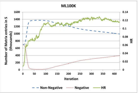
and then setting the smaller values to zero. One systematic way of doing this is to selectively retain only those non-zero entries which contribute the most to the length of the item similarities vector represented by the column in Sto which the entry belongs. The impact of this sparsification is further explored in the experimental results.
5.3
Results
The experimental evaluation consists of two parts. First, the effect of various model pa-rameters ofFISMon the recommendation performance is studied. Specifically, how bias, induced sparsity, estimation approach and non-negativity affects the top-N performance is studied. These studies are presented only on the ML100K-3 (represented as ML100K), Yahoo-2 (represented as Yahoo) and Netflix-3 (represented as Netflix) datasets. How-ever the same results and conclusions carry over to the rest of the datasets as well. These datasets are chosen to represent the datasets from different sources and at differ-ent sparsity levels. Unless specified all results in the first set of experimdiffer-ents are based on FISMrmse. Second, the comparison results with other competing methods (Section 4.4) on all the datasets is presented. The performance ofFISMis also compared for different values of N (as in top-N) and finally the performance ofFISMis compared with respect to data sparsity.
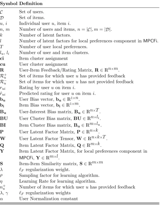
5.3.1 Effect of Bias
In FISM’s model, the user and item biases are learned as part of the model. In this study we compare the influence of user and item biases on the overall performance of the model. We compare the following four different schemes, N oBias - where no user or item bias is learned as part of the model, U serBias - only the user bias is learned,
ItemBias - only the item is learned andU ser&ItemBias- where both user and item biases are learned. The results are presented in Table 5.1. The results indicate that the biases affect the overall performance, with item bias leading to the greatest gains in performance.