LM-Tests for Linearity Against Smooth
Transition Alternatives: A Bootstrap Simulation
Study
∗
Jonathan B. Hill
†Dept. of Economics
Florida International University
July 5, 2004
Abstract
The universal method for testing linearity against smooth transition autoregressive (STAR) alternatives is the linearization of the STAR model around the null nuisance parameter value, and performing F-tests on poly-nomial regressions in the spirit of the RESET test. Polypoly-nomial regres-sors, however, are poor proxies for the nonlinearity associated with STAR processes, and are not consistent (asymptotic power of one) against STAR alternatives, let alone general deviations from the null. Moreover, the most popularly used STAR forms of nonlinearity, exponential and logis-tic, are known to be exploitable for consistent conditional moment tests of functional form, cf. Bierens and Ploberger (1997). In this paper, push-ing asymptotic theory aside, we compare the small sample performance of the standard polynomial test with an essentially ignored consistent con-ditional moment test of linear autoregression against smooth transition alternatives. In particular, we compute an LM sup-statistic and charac-terize the asymptotic p-value by Hansen’s (1996) bootstrap method. In our simulations, we randomly select all STAR parameters in order not to bias experimental results based on the use of "safe", "interior" parameter values that exaggerate the smooth transition nonlinearity. Contrary to past studies, we find that the traditional polynomial regression method performs only moderately well, and that the LM sup-test out-performs the traditional test method, in particular for small samples and for LSTAR processes.
1. Introduction Smooth Threshold Autoregressive (STAR) models have gained significant popularity in the economics andfinance literatures as a means
∗Key words: smooth transition autoregression; consistent conditional moment; bootstrap;
simulation
†Dept. of Economics, Florida International University, Miami, Fl; Fax: 305-348-1524;
to transcend well known estimation and forecasting limitations of both linear and binary switching (e.g. SETAR and Markov Switching) models. Original theoretical contributions belong to Tong (1983) and Chan and Tong (1986a,b), while Luukkonenet al (1988) and Teräsvirta (1994) develops a composite theory of estimation and testing for STAR processes with exponential and logistic tran-sition functions. Models of smooth regime switching have been widely applied to exchange rates, prices, and stock returns, and the general theory has been extended to the GARCH class of conditional volatility, and models offlexible parametric form. See Teräsvirta (1994) and van Dijket al (2000) for extensive bibliographies.
Consider a time series process {yt}, regressors xit = (1, yt−1, ..., yt−pi)0, i
= 1,2, and a stochastic shock ut. The class of two-regime STAR processes is
represented as
yt=φ01x1t+φ02x2tF(yt−d, γ, c) +ut, (1)
for some transition functionFt(d, γ, c) = F(yt−d, γ, c) :R3 →[0,1], transition
scaleγ >0, threshold variable yt−d,threshold c,and delay parameterd. The
transition function is assumed to be twice continuously differentiable inγ and
c. Luukkonen et al (1988), Teräsvirta (1994), and evidently the vast major-ity of applied research, consider logistic and exponential transition functions, respectively
Ft(d, γ, c) =
1
1 +e−γ(yt−d−c), Ft(d, γ, c) = 1−e
−γ(yt−d−c)2. (2)
If the scale parameterγ and/or vector φ2 are zero, then the process collapses to a linear autoregression.
Tests for linearity against STAR alternatives, however, have received little attention, and to date there do not exist treatments of consistent (asymptotic power of one) test methods. Under the traditional null hypothesis of linearity,γ
= 0, the coefficientsφ2 are unidentified, and therefore standard Lagrange Mul-tiplier statistics cannot be directly computed. Luukkonenet al (1988), Saikko-nen and LuukkoSaikko-nen (1988), Teräsvirta (1994), Hagerud (1997), Gonzalez-Rivera (1998), Escribano and Jorda (2000), Madieros and Veiga (2000) and others pro-scribe a truncated Taylor expansion approximation of the nonlinear transition functionFt(d, γ, c) aroundγ = 0 as a means to transcend the nuisance
para-meter and non-standard distribution dilemma. The technique leads to a simple polynomial auxiliary regression in the spirit of the RESET tests by Ramsey and Schmidt (1976) and Keenan (1985), and standardF-tests of parametric zero-restrictions. Tests on subsets of coefficients can be used to infer whether the process is exponential or logistic STAR. The simplicity of the auxiliary regres-sion makes this method employable in any standard econometrics software and therefore has appeal for quick applications.
Several fundamental problems associated with polynomial regressions exist, however. First, by construction the resultingF-tests do not necessarily lead to a STAR model when the null of linearity is rejected,unless it is assumed a priori
that the true data generating structure is STAR: see Teräsvirta (1994). The polynomial test amounts to a test of linearity on an assumed STAR process, and is not, therefore, a true test of smooth transition nonlinearity. To date, there does not exist a test which can reveal whether STAR nonlinearity pro-vides a better approximation to the true data generating structure than the null specification. Pending evidence in favor of a smooth transition structure improving modelfit, the polynomial regression would only then be appropriate for ascertaining which STAR model, exponential or logistic, best describes the data.
The polynomial regression technique only provides maximal power against local polynomial alternatives. This issue is particularly relevant if we admit
any functional alternative to explain the data provided linearity is found inad-equate, and are willing to use smooth transition nonlinearity to improve model performance1. Indeed, polynomial nonlinearity is knownnot to be ”generically comprehensive” in the sense that if linearity is incorrect, additive polynomial terms may not improve the modelfit: see Stinchcombe and White (1998). This shortcoming of classic weight-based moment condition specification tests is well known in the inference theory and artificial neural network literatures: see, e.g., Holley (1982), Davies (1987), Bierens (1990), and Kuan and White (1994).
Interestingly, the very nonlinear forms popularly espoused in the smooth transition literature, exponential and logistic, are generically comprehensive2.
Orthogonality tests (e.g. a score test) which incorporate such functional weights have been shown to obtain asymptotic power of one against arbitrary devia-tions from the null functional specification: see Bierens (1982, 1990), Bierens and Ploberger (1997), and Stinchcombe and White (1998). While the laudable property of such structure absorption has been long recognized in the applied neural network literature, it has evidently been ignored entirely in the STAR literature. Indeed, under general conditions it is straightforward to show ifFt(·)
is generically comprehensive, then so isxtFt(·). Thus, whereas a Bierens-type
test employs the scalar weightFt(·)and leads to a neural-network type model
when the null is rejected, use of the weightxtFt(·) in is identically generically
comprehensive and leads to a smooth transition type model when the null is rejected.
Second, for STAR tests based on one threshold variable yt−d, the ”delay”
parameter d still exists in the polynomial regression. The delay parameter
1This is precisely the spirit in which the consistent parametric tests developed by Bierens
(1990), Leeet al (1993) and Bierens and Ploberger (1997) are employed in neural network
modeling. A null specification is tested without a prior alternative in mind, while rejection
leads to a model with an additional neural network term that is guaranteed asymptotically to
improve the modelfit with probability one. See also Kuan and White (1994) and Stinchcombe
and White (1998). The Hausman, RESET and McLeod-Li tests are well known examples of
tests of model specification which are not consistent against general deviations, while
consis-tent nonparametric tests typically do not provide a parametric alternative when the null model
is found to be mis-specified: see, e.g., Yatchew (1992), Wooldridge (1992), Zheng (1996), and
Hong and White (1995)..
2In general, essentially any real analytic function is generically comprehensive, including
does not influence the process under the null, hence it must be treated as a nuisance parameter. Teräsvirta (1994) and many others suggest performing the polynomial regression tests for various delay values, sayd, and selecting thatd
which generates the lowest test p-value. This is mathematically equivalent to generating an LM sup-statistic over possibled-values, a statistic known to have a non-standard limit distribution. Nevertheless, in the literature the standard practice is simply to employp-values derived from the chi-squared distribution. Here, we abstract from asymptotic theory and focus entirely on small sam-ple performance of a class of tests universally over-looked in the above smooth transition literature. In a broad simulation study of linear AR, STAR and bi-linear processes, we employ Hansen’s (1996) method for approximating the null distribution of an LM sup-statistic based on the sample null score, and demon-strate the superior strengths of the resulting hybrid test method. Of separate interest, our simulation study also provides a rare glimpse into the comparative strengths of Bierens’ (1990) and Hansen’s (1996) competing solutions to the dilemma of asymptotic non-standard null distributions: we demonstrate that while a Bierens-type test for model specification against STAR alternatives pro-vides optimal power, Hansen’s (1996)p-value method is the best technique for analyzing the test statistic’s distribution for arbitrary sample sizes. Indeed, the combined LM sup-test with bootstrappedp-values typically dominates the pop-ularly espoused polynomial regression test for STAR processes, in particular for logistic STAR processes, and in general for STAR processes "far" from linear. Moreover, in many cases the STAR test dominates the Bierens test and the popularly employed neural test of "neglected nonlinearity", cf. Leeet al (1993), for detection of general model mis-specification.
Of particular note, our simulation study is substantially less restrictive than previous such studies: we do notfixanySTAR parameters, and therefore control for the fact thata priori chosen parameters may bias test results (e.g. Luukko-nen et al, 1988, Teräsvirta, 1994, Skalin, 1998). Wefind over a broad range of admissible STAR parameter values that a sup-LM statistic out-performs extant tests of STAR and general nonlinearity.
Finally, Skalin (1998) considers a Likelihood Ratio test of STAR nonlinear-ity in a simulation based environment, and employs Hansen’s (1996) bootstrap method for approximating the asymptoticp-value. The author finds the poly-nomial regression method dominates the bootstrapped LR statistic. Contrary to a score test, an LR test requires estimation of a specific alternative model. Even when using efficient maximum likelihood estimation, STAR models are renowned for their difficulty to provide sharp estimates of imperative transition function coefficients. Typically the imperative scale parameterγ estimate, on which the LR test hinges, appears to be insignificant, even in controlled ex-periments where the data generating structure is STAR: see Teräsvirta (1994) and Franses and van Dijk (2000). Thus, the power of such a test should be held suspect, and it is not surprising, therefore, that Skalin (1998)finds the LR test to be dominated by the provably non-consistent polynomialF-test method. Moreover, apparently the only consistent parametric tests of functional form be-long to the class of conditional moment tests developed in Bierens (1982, 1990)
and Bierens and Ploberger (1997) which lends itself specifically to an LM test framework. Because it is this class of tests that can be employed for a consistent test of linear autoregression against smooth transition alternative, we ignore LR tests.
The rest of this paper contains the following topics. In Section 2 the sup-LM test is outlined, and the simulation study is performed in Section 3. Tables can be found in the appendix.
2. Lagrange Multiplier Sup-Test Consider a standard two-regime STAR model:
yt=φ01x1t+φ20x2tFt(d, γ, c) +ut. (3)
For simplicity of notation, assume regressors are identical across regimes, x1t
= x2t = xt, a k × 1 vector. The fundamental null hypothesis of linearity
maintained throughout states
H0:φ2= 0. (4)
Under the null hypothesis, therefore,
yt=φ01xt+ t, (5)
where t=ut.Under the null, the transition parametersγ, c,anddare
unspec-ified: the hypothesis holds for any values, and therefore we treat the transition parameters as nuisance parameters.
Alternatively, whenγ = 0, the transition function is a constant (0 for the exponential, and1/2for the logistic) and the STAR model collapses to a linear AR model, for any value of φ2, c, and d. The hypothesis H0 : γ = 0 is the
favored focal point in the STAR test literature. Here, we focus on (8), and develop an associated LM statistic.
Denote by θthe vector of all parameters(φ01, φ02, d, γ, c)0. For compactness,
define the sub-vectorϕ= (d, γ, c)0. It is straightforward to show that the null
score obtains the representation
sn(θ)|H0=sn(0, ϕ) = · n−1Pn t=1 txt n−1Pn t=1 txtFt(ϕ) ¸ . (6)
Using least squares estimates from the null model, we obtain
ˆ sn(0, ϕ) = n−1 Xn t=1ˆtxtFt(ϕ) (7) = n−1Xn t=1ˆtzt ˆt = yt−ˆφ 0 1xt, zt=xtFt(ϕ).
The LM statistic, therefore, satisfies
where standard asymptotic algebra shows (see, e.g., Bierens, 1990) ˆ V(ϕ) = 1 n Xn t=1ˆ 2 t h Ft(ϕ)Ik−ˆb(ϕ) ˆA−1 i0 xtx0t h Ft(ϕ)Ik−Aˆ−1ˆb(ϕ) i (9) ˆb(ϕ) = 1 n Xn t=1Ft(ϕ)xtx 0 t, Aˆ= 1 n Xn t=1xtx 0 t,
andIk denotes thek-dimensional identity matrix.
Finally, define the sup-statistic,
gn= supϕTn(ϕ), (10)
where the supremum is taken over feasible values of the coefficient vector, ϕ= (d, γ, c)0: see below for details.
3. Simulation Study We now investigate the empirical size and power properties of the STAR sup-statisticgn= supTn(ϕ).Our simulations are based
on the following models:
H0:yt=φ01xt+ t
H1L:yt=φ01xt+φ02xt(1 + exp[−γ(yt−d−c)])−1+ t
H1E:yt=φ01xt+φ02xtexp[−γ(yt−d−c)2] + t
H1BL:yt=φ01xt+yt−1 t−1+ t
where t is iid standard normal3, and xt = (1, yt−1, ..., yt−p)0 for some p > 0.
UnderH0the true data generating process is linear; underH1L andH1E the true
process is a 2-regime LSTAR and ESTAR, respectively; underHBL
1 the process
is a hybrid bilinear-autoregression.
3.1 Set-up We consider sample sizesn= 100,500,and1000: in each case, we generate3n observations, and retain the last n observations in order to reduce dependence on starting values. For each simulated series, the orderp
is randomly chosen from the set{1, ...,10}, andφis randomly chosen from the uniform hypercube[−1.5,1.5]p+1.Moreover, the scale parameterγ is randomly selected from the uniform interval[.05,5], the thresholdcis randomly selected from[−.5, .5], and delaydis randomly chosen from the integer set {1, ..., p}. Be-cause typical asymptotic considerations require the null model to be covariance stationary, only vectorsφ1with characteristic polynomial roots outside the unit circle are considered.
We generate 1000 replications of each series above. For each series, a linear model is estimated and the resulting residuals are tested at the 5%-level. In order to specify the null model, we employ a minimum AIC model selection criterion for the orderpover the integer set{1, ...,10}.
3All simulations are performed using the GAUSS 5.0 software. Code is available upon
3.2 Tests In order to test for linearity, consider model (3). The STAR sup-LM test is based on the score weightzt =xtFt(ϕ), cf. (7).The test is
per-formed based on grid-searches overd, γ, andc. Following the standard rule of thumb (see, e.g., Teräsvirta, 1994), possible threshold values c are limited to the interval between the lower and upper15th-quantiles ofy
t, denotedy[.15]and
y[.85]. Moreover, forγwe search over the interval[.1,10], and the candidate delay
values are restricted to the interval set{1,2,3}.Although the simulated STAR series use a randomly selected scale γ with lower bound .05, the tests them-selves must use a larger lower bound (.10) due to covariance matrix singularity for small samples: the weightxtFt(ϕ)≈xt×ζ for some scalar-constantζ >0
whenγis close to zero, in which case the asymptotic covariance matrix estimator
ˆ
V(ϕ)becomes singular due to machine error. We use both Bierens’ (1990) cri-terion technique for generating an asymptoticχ2-statistic, and Hansen’s (1996)
simulatedp-value method in other to approximate the true null distribution of
gn.
Bierens’ (1990) criterion technique for generating an asymptotically χ2 -statistic is performed as follows. Letϕ∗ = arg max
ϕTn(ϕ), and letϕ˜denote a
nuisance vector randomly selected independent of the sample of data. Define the respective LM statisticsTn(ϕ∗)and Tn(˜ϕ). For arbitrary parameters ψ >
0andρ∈(0,1), we selectϕˆ such that
ˆ
ϕ = ϕ˜ ifTn(ϕ∗)−Tn(˜ϕ)≤ψnρ
ˆ
ϕ = ϕ∗ ifT
n(ϕ∗)−Tn(˜ϕ)> ψnρ.
Under H0 and appropriate assumptions governing dependence, the resulting
statisticTn(ˆϕ)converges in law to aχ2-random variable with k-degrees of
free-dom: see Bierens (1990: Theorems 4-5).In lieu of simulation evidence reported in Bierens (1990), we useψ=.25andρ=.5. This is theSTAR_Bier test.
Hansen’s (1996) method involves simulating the null distribution of the sup-scoreˆs(0, ϕ∗), whereϕ∗= arg maxϕTn(ϕ). We drawn×Jiid random variables
ut,j ˜N(0,1),t= 1...n, j = 1...J,and generate a sample ofJ-scores andJ-test
statistics: ˆ sn,j(0, ϕ∗) = 1 n Xn t=1ˆtxtFt(ϕ ∗)u t,j (11) Tn,j(ϕ∗) = nsˆn,j(0, ϕ∗)0Vˆ(ϕ∗)−1sˆn,j(0, ϕ∗).
The approximate p-value of the sup-statistic gn is simply the frequency with
whichTn,j(ϕ∗)> gn occurs. For all simulations, we setJ = 500. This is the
STAR_han test.
We also perform the neural test of neglected nonlinearity (Lee et al,1996), the Bierens test, the McLeod-Li test, the RESET test, and the polynomial regression test of Luukkonenet al (1988) and Teräsvirta (1994).
The Bierens test is similar to the STAR test, except the scalar weightzt =
Ft(ϕ)is used. In this sense, we can simply interpret the Bierens test as a test
against a restricted STAR process with second regime slopes equal to zero: see also Franses and van Dijk (2000) on a related point. For the Bierens test, we
employ both Bierens’ (1990) criterion, withψ=.5andρ=.25(BIER); and we use Hansen’s (1996) method for evaluating the true distribution of the Bierens sup-statistic (BIER_han). In this manner, we control for the possibility that differences between the STAR sup-test and all other tests is merely due to the use of Hansen’s (1996) method.
The neural test is equivalent to the Bierens test (i.e. zt = Ft(ϕ)), except
all nuisance parametersd, γ, andcare randomly selected from their respective intervals, detailed above.
For the standard STAR polynomial test, we estimate models of the form
yt=φ01x1t+
XL
i=1β
0
ix˜tyit−1+ut, (12)
wherex˜t = (yt−1, ..., yt−p). Under a null of linearity against an LSTAR
alter-native,L= 3and (12) impliesβi = 0,i= 1..3.Under a null of linearity against an ESTAR alternative, L = 4 and (12) implies βi = 0, i = 1..4. In order to decide between LSTAR and ESTAR alternatives based on the polynomial re-gression, Teräsvirta (1994) suggests a test ofH0:βi = 0,i= 1..4first in order
to substantiate concern for STAR nonlinearity at all, then a sequence ofF-tests on parameter sub-sets from (12). Because we are interested in whether the test procedure canfindany deviation from the null of linearity, we do not pursue the test sequence approach and simply report null rejection frequencies based on tests of (12) withL= 3or4. Rejection in either case is argued to be consistent with evidence in favor of STAR nonlinearity, cf. Luukkonenet al (1988). These are thePOLY_LandPOLY_E tests, respectively.
For the McLeod-Li test, we perform a standard portmanteau test on the squared null residuals for lags1...3.For the RESET test, we follow the procedure detailed in Thursby and Schmidt (1977) by estimating the auxiliary regression based on the null residualsuˆt,
ˆ ut=β00xt+ XL i=2 Xk j=2βi,jx i t,j+wt, (13)
where we setL = 3.A standard LM test for the linearity hypothesis H0 : βi,j
= 0is performed.
For all LM tests employed in this study, covariance matrix estimators robust to unknown forms of conditional heteroscedasticity are used.
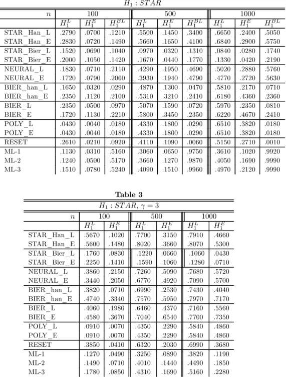
3.3 Results Test results for H0 are contained in Table 1, and
Ta-ble 2 contains empirical powers for LSTAR, ESTAR and bilinear alternatives. For linear processes, the STAR tests compare well with the popularly used neural and polynomial regression tests. The polynomial and STAR tests tend to under-reject the null, while only the neural and exponential Bierens tests closely approach the 5% level.
Under an LSTAR alternative, the STAR tests evaluated by bootstrapped
p-values dominate all other tests for sample sizes of100and500. For largen= 1000the STAR test only slightly out-performs the polynomial regression tests,
yet still dominates all other tests. Under an ESTAR alternative, by comparison, the STAR tests do not perform as favorably as the polynomial regression test, however all tests, except the Bierens test, generate relatively low empirical re-jection frequencies. The Bierens test with an exponential weight is more adept at detecting linear model mis-specification in the presence of true ESTAR non-linearity than the polynomial regression test. This also suggests in practice that a neural network model may be found to improve model performance even when the traditional STAR test suggests a linear model in adequate.
In general, the use of Bierens’ (1990) criterion method is dramatically sub-optimal for the STAR sup-test, but not the Bierens test. Of course, the problem may simply be due to thefixed criterion parameters values forψandρ. In any event, our simulations strongly suggest Hansen’s (1996) bootstrappedp-value method for the STAR test renders a highly competitive test method, however does not improve the performance of the Bierens test. Because bootstrapped
p-values are increasingly de riguer in practice, and because they impressively aid STAR test performance here, we do not consider other values ofψandρ.
Moreover, the Bierens test, even when analyzed by bootstrapped p-values, is substantially out-performed by the STAR and neural tests for tests on bi-linear processes, the class of processes used in the simulation study of Bierens (1990). The McLeod-Li test, however, has optimal power against Gaussian bi-linear processes (see McLeod and Li, 1983), hence it is not surprising how well the test performs in our study. For STAR nonlinearity, however, the McLeod-Li test is outperformed by the Bierens, neural and in particular the STAR tests.
Recall that we randomize the transition scaleγ∈[.05,5]for STAR processes. Values closer to zero imply a STAR model with very slow regime transition such that the process appears to be "nearly linear". Thus, our simulation study demonstrates that over a broad spectrum of transition velocities the sup-LM test dominateson average the polynomial regression method, in particular against LSTAR alternatives. However, the sup-LM statistic used in the present study is shown by Andrews and Ploberger (1994) to be the limit of an optimal test (admissible for any alternative, hence any non-zero value of φ2 and γ), and
effectively directs power toward distant deviations from the null. Thus, despite being asymptotically consistent against any deviation from the null, the statistic is expected to provide more power against deviations "far" from linearity (i.e. largeγ) for small samples.
We check this by performing an identical simulation study of only STAR processes with a fixed γ = 3. All other simulation specifications remain as above. Results are contained in Table 3. For STAR process that are more "distant" from a linear autoregression, the sup-LM test demonstrates its com-parative power lift both relative to itself when performed on STAR processes that may be "nearly linear", and relative to the polynomial regression method. Using bootstrappedp-values and forn≥500, the STAR test with either expo-nential of logistic weightsxtFt(ϕ)correctly detects LSTAR nonlinearity in over
77% of such series, while the polynomial test correctly rejects the null in favor of STAR in 43.50% (58.40%) series with sample size 500 (1000). Of particular note, the STAR tests improved on empirical power for smalln= 100by nearly
30% relative to simulations with randomizedγ, while the polynomial F-test re-sults in about 5% more power, admittedly an increase of over 100% relative to the previous rejection rate with a randomized scaleγ. However, even the RE-SET test performs better than the standard polynomial STAR test for "strong" STAR processes. In general, using either an exponential or logistic weight the STAR sup-LM test dominates all tests when the true process is LSTAR.
Not only does the STAR test provide power leverage against unknown arbi-trary deviations from the null (e.g. possibly smallγand bilinear nonlinearity), but against strong forms of smooth transition nonlinearity (i.e. large γ) and in particular against logistic STAR nonlinearity. The present simulation study persuasively demonstrates that the universally employed polynomial STAR test is sub-optimal relative to a sup-LM test, as well as the consistent Bierens and neural tests. Indeed, the polynomial test may not even be an appropriate test methodology for detecting which STAR form, exponential or logistic, best ap-proximates the true data generating process. We may well argue that the best test approach is a consistent STAR test of linear autoregression against either STAR form, where the subsequent decision between STAR forms is informed by economic theory and policy considerations.
Appendix
Table 1 H0:AR(p) n 100 500 1000 STAR_Han_L .0330a .0040 .0010 STAR_Han_E .0360 .0070 .0030 STAR_Bier_L .0580 .0140 .0060 STAR_Bier_E .0840 .0340 .0130 NEURAL_L .0390 .0460 .0440 NEURAL_E .0390 .0590 .0390 BIER_han_L .0110 .0240 .0180 BIER_han_E .0400 .0580 .0430 BIER_L .0170 .0260 .0150 BIER_E .0420 .0470 .0490 POLY_L .0010 .0030 .0020 POLY_E .0010 .0030 .0020 RESET .0450 .0380 .0490 ML-1b .0520 .0700 .0860 ML-2 .0570 .0880 .0910 ML-3 .0640 .1050 .0950Notes: a. p-values less than .00005 are reported as .0000; b.ML-h denotes the ML test with h-lags.
Table 2 H1:ST AR n 100 500 1000 HL 1 H1E H1BL H1L H1E H1BL H1L H1E H1BL STAR_Han_L .2790 .0700 .1210 .5500 .1450 .3400 .6650 .2400 .5050 STAR_Han_E .2830 .0720 .1490 .5660 .1650 .4100 .6840 .2900 .5750 STAR_Bier_L .1520 .0690 .1040 .0970 .0320 .1310 .0840 .0280 .1740 STAR_Bier_E .2000 .1050 .1420 .1670 .0440 .1770 .1330 .0420 .2190 NEURAL_L .1830 .0710 .2110 .4290 .1950 .4690 .5020 .2880 .5760 NEURAL_E .1720 .0790 .2060 .3930 .1940 .4790 .4770 .2720 .5630 BIER_han_L .1650 .0320 .0290 .4870 .1300 .0470 .5810 .2170 .0710 BIER_han_E .2350 .1120 .2100 .5310 .3210 .2410 .6180 .4360 .2360 BIER_L .2350 .0500 .0970 .5070 .1590 .0720 .5970 .2350 .0810 BIER_E .1720 .1130 .2210 .5800 .3450 .2350 .6220 .4670 .2410 POLY_L .0430 .0040 .0180 .4330 .1800 .0290 .6510 .3820 .0180 POLY_E .0430 .0040 .0180 .4330 .1800 .0290 .6510 .3820 .0180 RESET .2610 .0210 .0920 .4110 .1090 .0060 .5150 .2710 .0010 ML-1 .1130 .0310 .5160 .3060 .0650 .9750 .3610 .1020 .9920 ML-2 .1240 .0500 .5170 .3660 .1270 .9870 .4050 .1690 .9990 ML-3 .1510 .0780 .5240 .4090 .1510 .9960 .4970 .2120 .9990 Table 3 H1:ST AR, γ= 3 n 100 500 1000 HL 1 H1E H1L H1E H1L H1E STAR_Han_L .5670 .1020 .7700 .3150 .7910 .4660 STAR_Han_E .5600 .1480 .8020 .3660 .8070 .5300 STAR_Bier_L .1760 .0830 .1220 .0660 .1060 .0430 STAR_Bier_E .2250 .1410 .1590 .1060 .1280 .0710 NEURAL_L .3860 .2150 .7260 .5090 .7680 .5720 NEURAL_E .3440 .2050 .6770 .4920 .7090 .5700 BIER_han_L .3820 .0710 .6990 .2530 .7430 .4040 BIER_han_E .4740 .3340 .7570 .5950 .7970 .7170 BIER_L .4060 .1980 .6460 .4370 .7160 .5560 BIER_E .4580 .3670 .7040 .6540 .7700 .7350 POLY_L .0910 .0070 .4350 .2290 .5840 .4860 POLY_E .0910 .0070 .4350 .2290 .5840 .4860 RESET .3850 .0410 .6320 .2030 .6990 .3680 ML-1 .1270 .0490 .3250 .0890 .3820 .1190 ML-2 .1490 .0710 .4010 .1440 .4490 .1850 ML-3 .1780 .0850 .4310 .1690 .5160 .2280
References
[1] Bierens, H. J., 1982, Consistent Model Specification Tests, Journal of Econometrics 20, 105-134.
[2] Bierens, H. J., 1990, A Consistent Conditional Moment Test of Functional Form, Econometrica 58, 1443-1458.
[3] Bierens, H. J. and W. Ploberger, 1997, Asymptotic Theory of Integrated Conditional Moment Tests, Econometrica 65, 1129-1151.
[4] Chan, K.S. and H. Tong, 1986b, On Tests for Nonlinearity in Time Series Analysis, Journal of Time Series Analysis 5, 217-228.
[5] Davies, R.B., 1987, Hypothesis Testing When a Nuisance Parameter is Present Only under the Alternative, Biometrika 74, 33-43.
[6] van Dijk, D., T. Teräsvirta and P.H. Franses, 2000, Smooth Transition Autoregressive Models-A Survey of Recent Developments, Econometric In-stitute Research Report EI2000-23/A, Erasmus University.
[7] Escribano, A. and O. Jordá, 1999, Improved Testing and Specification of Smooth Transition Autoregressive Models, in P. Rothman (ed.), Nonlinear Time Series Analysis of Economic and Financial Data, pp. 289-319 (Boston: Kluver).
[8] Gonzalez-Rivera, G., 1998, Smooth-transition GARCH models, Studies in Nonlinear Dynamics and Econometrics 3, 61-78.
[9] Hagerud, G.E., 1997, A New Nonlinear GARCH Model, Unpublished Ph.D. thesis, IFE, Stockholm School of Economics.
[10] Hansen, B., 1996, Inference When a Nuisance Parameter Is Not Identified Under the Null Hypothesis, Econometrica 64, 413-430.
[11] Holley, A., 1982, A Remark on Hausman’s Specification Test, Econometrica 50, 749-760.
[12] Hong, Y. and H. White, 1995, Consistent Specification Testing via Non-parametric Series Regression, Econometrica 63, 1133-1159.
[13] Keenan, D.M., 1985, A Tukey Nonadditivity-Type Test for Time Series Nonlinearity, Biometrika 72, 39-44.
[14] Kuan, C. and H. White, 1994, Artificial Neural Networks: An Economic Perspective, Econometric Reviews 13, 1-91.
[15] Lee, T., H. White and C.W.J. Granger, 1993, Testing for Neglected Nonlin-earity in Time-Series Models: A Comparison of Neural Network Methods and Alternative Tests, Journal of Econometrics 56, 269-290.
[16] Luukkonen, R., P. Saikkonen and T. Teräsvirta, 1988, Testing Linearity against Smooth Transition Autoregressive Models, Biometrika 75, 491-9. [17] Madieros, M.C. and A. Veiga, 2000, Diagnostic Checking in a Flexible
Nonlinear Time Series Model, manuscript, Dept. of Electrical Engineering, Catholic University of Rio de Janeiro.
[18] Ramsey, J.B., and P. Schmidt, 1976, Some Further Results on the Use of OLS and BLUE Residuals in Specification Error Tests, Journal of the American Statistical Association 71, 389-390.
[19] Saikkonen, P. and R. Luukkonen, 1988, Lagrange Multiplies Tests for Test-ing Nonlinearities in Time Series Models, Scandinavian Journal of Statistics 15, 55-68.
[20] Skalin, J., 1998, Testing Linearity against Smooth Transition Autoregres-sion Using A Parametric Bootstrap, Working Paper Series in Economics and Finance No. 276, Dept. of Economic Statistics, Stockholm School of Economics.
[21] Stinchcombe, M.B. and H. White, 1998, Consistent Specification Testing with Nuisance Parameters Present Only Under the Alternative, Economet-ric Theory 14, 295-325.
[22] Teräsvirta, T., 1994, Specification, Estimation, and Evaluation of Smooth Transition Autoregressive Models, Journal of the American Statistical As-sociation 89, 208-218.
[23] Thursby, J., and P. Schmidt, 1977, Some Properties of Tests for Specifi ca-tion Error in a Linear Regression Model, Journal of the American Statistical Association 72, 635-641.
[24] Tong, H., 1983, Threshold Models in Non-Linear Time Series Analysis (New York: Springer-Verlag).
[25] Wooldridge, J., 1991, On the Application of Robust, Regression- Based Diagnostics to Models of Conditional Means and Conditional Variances, Journal of Econometrics 47, 5-46.
[26] Yatchew, A.J., 1992, Nonparametric Regression Tests Based on Least Squares, Econometric Theory 8, 435-451.
[27] Zheng, J., 1996, A Consistent Test of Functional Form via Nonparametric Estimation Techniques, Journal of Econometrics 75, 263-289.