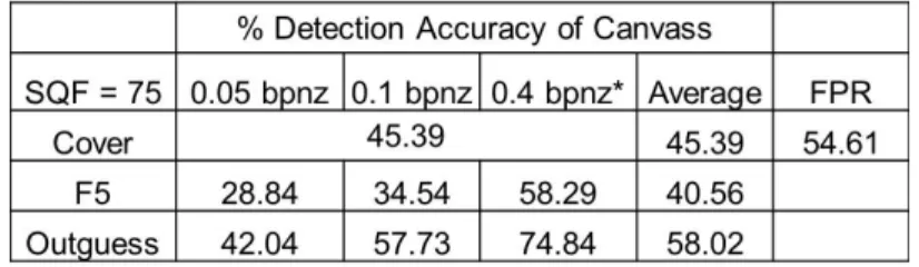
A Canvass steganalyzer for double-compressed JPEG images

When financial statements are prepared by Company A at the end of December 2018, the taxable temporary difference originating in 2017 reverses, resulting in an increase

Role of Peer Counseling on the Relationship between Prefects and the Students’ body in public Secondary schools in Migori Sub-county, Migori County, Kenya

This unique event will appeal to public officials who are charged with motivating employees to provide the highest level of customer-oriented service, promoting productivity

Up until 72 hours before fight time I like to feed in the cock house both morning and night, have him roost there, but spend the day outside whenever

The comparison of the differences between SCIAMACHY and the two MIPAS measurement periods (Figs. 3 and 11), shows that at the lower altitudes MIPAS produces slightly higher

2. A good friend is one who to some extent shares our suffering when we ourselves are miserable. We would not want someone as a friend who.. The Big Picture: Divine

26.2 Appliances having type X attachment and for connection to fixed wiring shall be provided with terminals, unless the connections are soldered. Screws, nuts serve only for

III e V Compounds such as gallium arsenide (GaAs), indium phosphide (InP) and gallium antimonide (GaSb) have direct energy bandgaps, high optical absorption coefficients and good