Partially Occluded Object Detection

i

PARTIALLY OCCLUDED OBJECT DETECTION

by Di Sun

B.S. in Electrical Engineering, Beijing Jiaotong University, Beijing, China, 2014

Submitted to the Graduate Faculty of

Swanson School of Engineering in partial fulfillment of the requirements for the degree of

Master of Science

University of Pittsburgh 2016

UNIVERSITY OF PITTSBURGH SWANSON SCHOOL OF ENGINEERING

This thesis was presented

by

Di Sun

It was defended on March 29, 2016 and approved by

Chen, Yiran, PhD, Associate Professor, Department of Electrical and Computer Engineering Li, Ching-Chung, PhD, Professor, Department of Electrical and Computer Engineering Li, Hai, PhD, Associate Professor, Department of Electrical and Computer Engineering

Thesis Advisor:

iii

Copyright © by Di Sun 2016

Object detection is a fairly important field in computer vision and image processing, and there are some domains that have been well researched, such like face detection and pedestrian detection, while these detections are based on situation that there are no shelters on objects in images or videos. But most objects are partially occluded in real world. And this becomes one major obstacle in object detection. In this paper, I utilize a state-of-art model, Deformable Part Model (DPM), which present a mixture model contains multi-scale deformable parts. And attach visibility flags to both cells and part of it. A visibility flag is used to indicate whether a specific cell or part is visible or occluded. By removing the contribution of occluded cells and parts to the whole detection score, the performance of partially occluded object detection can be significantly improved. To get the value of visibility flags, I use a mathematical method called Alternating Direction Method of Multipliers (ADMM). The experiment shows that by using this model, the detection accuracy of partially occluded object is improved.

PARTIALLY OCCLUDED OBJECT DETECTION

Di Sun, M.S.

v

TABLE OF CONTENTS

TABLE OF CONTENTS ... V LIST OF TABLES ... VII LIST OF FIGURES ... VIII

1.0 INTRODUCTION ... 1

2.0 RELATED WORK ... 6

3.0 PROBLEM BACKGROUND ... 8

3.1 HISTOGRAMS OF ORIENTED GRADIENTS ... 8

3.1.1 Implementation of Algorithm ... 9

3.2 ALTERNATING DIRECTION METHOD OF MULTIPILER ... 10

3.2.1 Implementation of Algorithm ... 10

4.0 PART BASED MODEL ... 12

4.1 MODEL ... 12

4.1.1 Deformable Part Models ... 14

4.1.2 Matching ... 15

4.1.3 Mixture Model ... 16

4.2 LSVM ... 18

4.2.1 Semi-convexity... 18

4.3 TRAINING ... 20 4.3.1 Learning Parameter... 20 4.3.2 Initialization... 23 5.0 OCCLUSION HANDLING ... 25 5.1 MODEL ... 25 5.2 IMPLEMENTATION ... 28 6.0 EXPERIMENTS ... 29

6.1 DETECTION OF FULLY VISIBLE OBJECTS ... 29

6.2 DETECTION OF PARTIALLY OCCLUDED OBJECTS ... 32

7.0 CONCLUSION ... 38

vii

LIST OF TABLES

LIST OF FIGURES

Figure 1. Person detection model... 2

Figure 2. Two components car detection model ... 5

Figure 3. Image pyramid (left) and its corresponding feature pyramid (right) ... 13

Figure 4. Star model for bottle ... 14

Figure 5. Procedure of matching ... 17

Figure 6. Pseudo code of training process ... 22

Figure 7. Model for bicycle ... 24

Figure 8. Some model examples trained on PASCAL 2007 dataset ... 30

Figure 9. Some detection result on PASCAL test dataset ... 31

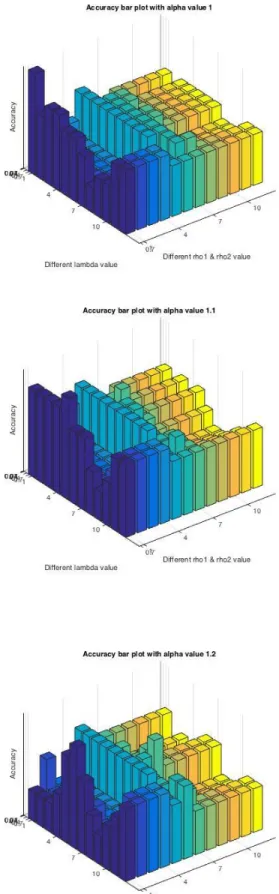
Figure 10. Alpha from 1 to 1.2 ... 33

Figure 11. Alpha from 1.3 to 1.5 ... 34

Figure 12. Alpha from 1.6 to 1.8 ... 35

1

1.0 INTRODUCTION

This paper introduces a method for object detection with partially occluded based on a state-of-art model, Deformable pstate-of-art models (DPM) [1]. The problem of detecting and localizing is a fundamental and important challenge in computer vision area. Detecting objects such as pedestrians and cars in static images is a tough problem because these objects, especially pedestrians, can vary significantly from image to image. Besides their poses and shapes, image illumination, complexity of background and viewpoint can also arise the variation. Despite significant effort has been put and encouraging development has been made recent years, most of them are only focus on detecting fully visible objects. When comes with objects with partial occlusion, the detection results are not good enough.

Most popular detection models use method of bounding box, which supposes that all pixels in the bounding box belong to the object. But in real world, not all objects are entirely visible, which means not all pixels support the object. For example, in the Galtech Pedestrian Dataset [22], at least 70% of pedestrian are partially or fully occluded in at least one frame of a video sequence. Dollar et al. [22] show that detection performance for standard methods drops significantly even under partial occlusion, and drastically under heavy occlusion. [6] So a detection model that can learn the visibility of pixels of an object is very important.

Method in this paper is based on a mixture Deformable Part Model, which provides an outstanding framework for the problem of object detection. Deformable part model can

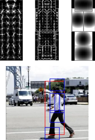
significantly capture the object variations, but using only one is not sufficient. Discriminatively Trained Deformable Part Model [1] uses a mixture of star-structured deformable part models, which contains a “root” filter and a set of part filters to better represent the variations on both pixel level and part level. Figure 1 shows a star-structured model for pedestrian.

3

At a specified position and scale, score of the star-structured model is the sum of responses of root filter and every part filter. The response of each filter is calculated by the dot product of filter weights and image features inside the detection window. In this model, part filters are applied to feature maps twice the resolution of root filters. By doing this, feature descriptors can better represent parts of objects and experiments show that by doing this, the detection performance is improved. However, datasets available now are all weakly labeled, which means there are labels only for root bounding box of an object. So we need a Support Vector Machine for Multiple-Instance Learning (MI-SVM) [17], in the following paper we will call it latent SVM (LSVM), to train the star-structured model with partially labeled dataset. We introduce a latent variable, which is used to indicate the positions of root and every part according to the object. The detection score of an input example x is calculated by the following form of function,

𝑓_𝛽 = max

𝑧∈𝑍(𝑥)𝛽 ∙ Φ(x, z)

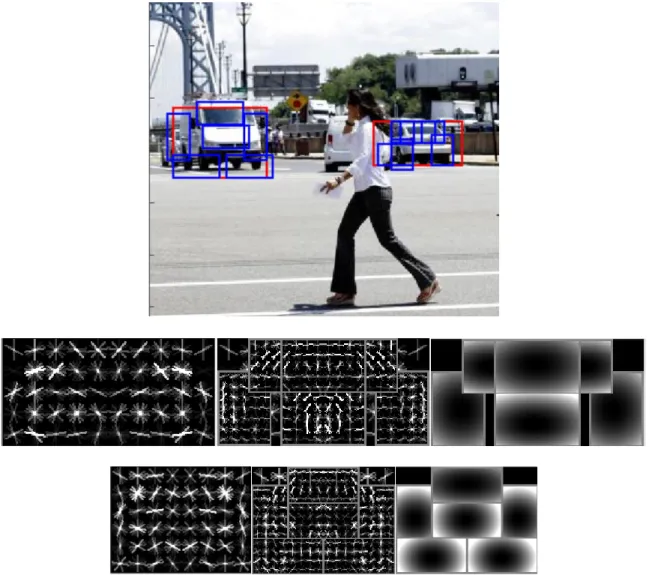
where 𝛽 is a vector of model parameters, z is the vector of latent values, and Φ(x, z) is feature vector. In the star-structured model, 𝛽 is the concatenation of the root filter weights, part filters weights and deformation cost weights, Φ(x, z) is the concatenation of feature pyramid image inside root filter and part filters detection windows according to the object. A model for a specified class consists of several star-structured models, each one of which represents a component. Figure 2 shows a model for cars with two components.

I attach latent visibility flags to part filters and every cell of root filter of deformable part model to deal with the detection of partially occluded objects. A visibility flag is a binary variable indicates whether the cell or part of a particular object is occluded or visible, 0 for occluded and 1 for visible. In order to get the value of visibility flags, I use an optimization

method called Alternating Direction Method of Multiplier (ADMM). Since we know that generally occluded parts of an object, especially pedestrian, are on the bottom and tend to cluster together, so the concave function we use to be maximized totally contains four parts: sum of the detection score of root filter and every part filter, a penalty term to encourage occluded parts appear at the bottom of the object, a consistency term to encourage cells concatenating have the same visibility flag, a consistency term to make sure that overlapped cells of root filter’s detection window and parts have the same visibility flag. Experiments show that by removing the contribution of occluded cells and parts to final detection score, the performance of partially occluded object detection is significantly improved.

5

2.0 RELATED WORK

In recent years, object detection without occlusion has significantly developed, and most of the methods can achieve a considerable accuracy rate. However, occlusion handling is still an obstacle in this area, and a lot of researchers address the problem of partially occluded object detection. Paper [4] combines the Histogram of Oriented Gradients (HOG) with Local Binary Pattern (LBP) to get the feature set. They use the response of each block in HOG feature vector to construct occlusion likelihood maps and classify them with Mean Shift approach. Paper [5] use latent variables to indicate the visibility of every cell, but the model they construct can only be used in the situation that the object is truncated. In real world most objects are occluded by other objects, so this method cannot solve common problems. Paper [6] provides a segmentation-aware object detection model. A latent variable is also attached to every cell in their model to indicate whether the cell belongs to the object. They construct a structural SVM to learn the values of latent variables, which means this model need to be trained with features of both objects being occluded and occluder. This will be time-consuming and the training dataset needed is also relatively large.

Models above are using holistic detectors, while Paper [7], [8], [8], [9] use part-based detectors instead of the whole object detector and attach visibility flags to every part. Like method in this paper, Paper [7] also based on deformable part model and use latent variable to indicate the visibility of every part. They construct a discriminate deep model to learn the

7

visibility relation shape of overlapping parts. Paper [8] use the contextual and spatial configuration information from deformable part model to train conditional random field (CRF) parameters and use stochastic gradient descent with belief propagation to optimize CRF to get visibility flag value. But all these methods only based on part detectors and ignore the occlusion information on finer cell level.

There are some other approaches like training occlusion specified dataset, which is quite time consuming. Paper [14] provides an approach to train a double person detector to handle person-to-person occlusion, which cannot be handling with in this paper.

3.0 PROBLEM BACKGROUND

3.1 HISTOGRAMS OF ORIENTED GRADIENTS

A good object detection method must base on a robust feature descriptor, which can greatly represent the object and make it discriminate from complex background. Edge and gradient based descriptors are most widely applied to object detection methods, and among theses approaches, grids of Histograms of Oriented Gradient (HOG) descriptors plays a very important role because its outstanding performance.

The basic idea of HOG is that local object appearance and shape can often be characterized rather well by the distribution of local intensity gradient or edge directions, even without precise knowledge of the corresponding gradient or edge position [2]. To implement this descriptor, we can divide the image inside detection window into small connected regions, which we called cells, and in each cell, we calculate centered horizontal and vertical gradient of every pixel in the cell and accumulate them together. The combination of these histograms represents the descriptor. Then by creating larger spatial regions (blocks) and accumulating “energy” inside the block, the local histograms can be contrast normalized to get better performance. This normalization will improve the descriptor’s robustness to illumination and shadow changes.

9 3.1.1 Implementation of Algorithm

The Algorithm implementation is consisted of four parts: gradient computation, orientation binning, creating blocks and block normalization.

The first step is to compute centered horizontal and vertical gradient and gradient’s orientation and magnitude. The most common method is to apply a centered point discrete derivative mask in horizontal and vertical directions. The two filter kernels are:

𝐷𝑥= [−1 0 1] 𝐷𝑦 = [1 0 − 1] 𝑇

The second step is to create cell histogram by casting weighted vote from every pixel, where vote can be the magnitude of gradient or square or square root of it. Histogram bins are evenly spread over 0 to 180 degrees or 0 to 360 degrees, which is depending on whether the gradient is “unsigned” or “signed”. After experiments, Dalal and Triggs [2] found that unsigned gradients use in conjunction with nine histogram bins performs best.

In order to make the descriptor robust to the change of illumination and image contrast, a local normalization should be applied to the gradients inside a block. Since generally these blocks are overlapped, cells in one block may contribute twice or more to the final descriptor. Many normalization factors like 𝑙₁ norm and 𝑙₂norm can be used here to do the block normalization. A created feature descriptor can be put into a classifier like linear SVM to train and get the final detector.

3.2 ALTERNATING DIRECTION METHOD OF MULTIPILER

In computer vision and machine learning area, many problems can be finally posed in a framework of convex function optimization. Due to the large size and high complexity of most dataset we needed in this area, a good optimization method becomes critical. Both computing time and storage of large data size should be taken into consideration when choosing an optimization approach. In this paper, I use a method called Alternation Direction Method of Multiplier (ADMM), which is well suited to distributed convex optimization, especially to large-scale problem. This method was developed in the 1970s, with roots in the 1950s, and is closely related to many other algorithms, such as dual decomposition, Doughlas-Rachford splitting, Spingran’s method of partial inverses, the method of multiplier and others.

3.2.1 Implementation of Algorithm

Here I will give a simple overview of ADMM. More details please refer to the [16]. Giving an example of optimizing a convex function 𝑓(𝑥).

𝑚𝑖𝑛𝑖𝑚𝑖𝑧𝑒 𝑓(𝑥)

𝑠𝑢𝑏𝑗𝑒𝑐𝑡 𝑡𝑜 𝑥 ∈ 𝐶 (3-1) here 𝑥 is input variable that subjects to condition set 𝐶, and 𝑓(𝑥) is a convex function. We can first rewrite the function to the following form,

𝑚𝑖𝑛𝑖𝑚𝑖𝑧𝑒 𝑓(𝑥) + 𝐼_𝐶(𝑧)

𝑠𝑢𝑏𝑗𝑒𝑐𝑡 𝑡𝑜 𝑥 = 𝑧 (3-2) where 𝐼_𝐶(𝑧) is the indicator function on 𝐶, which means 𝐼_𝐶(𝑧) = 0 for 𝑧 ∈ 𝐶 and 𝐼_𝐶(𝑧) = + ∞

11

𝐿_𝜌(𝑥, 𝑧, 𝑢) = 𝑓(𝑥) + 𝐼𝐶(𝑧) + 𝜌

2‖𝑥 − 𝑧 + 𝑢‖2

2 _(3-3) Where 𝑢 is a scaled dual variable associated with the constraint 𝑥 = 𝑧 and 𝜌 > 0 is penalty parameter. In each iteration, we perform alternation minimization of the augment Lagrangian function over 𝑥 and 𝑧 and update value following steps as below,

𝑥𝑘+1 _{≔ 𝑎𝑟𝑔𝑚𝑖𝑛 {𝑓(𝑥) +}𝜌 2‖𝑥 − 𝑧 𝑘_{+ 𝑢}𝑘_‖ 2 2_} 𝑧𝑘+1 _{≔ Π} 𝐶(𝑥𝑘+1+ 𝑢𝑘) 𝑢𝑘+1≔ 𝑢𝑘+ (𝑥𝑘+1− 𝑧𝑘+1) (3-4) When updating 𝑥, we fix 𝑧 and 𝑢. Similarly, when updating 𝑧, 𝑥 and 𝑢 are fixed and updating 𝑢

while 𝑥 and 𝑧 are fixed. Π_𝐶 denotes the Euclidean projection onto constrain set 𝐶. A typical criterion to stop the iteration is,

‖𝑒_𝑃𝑘‖₂ ≤ 𝜖𝑝𝑟𝑖, ‖𝑒_𝑑𝑘‖₂ ≤ 𝜖𝑑𝑢𝑎𝑙 (3-5) Where 𝑒_𝑃𝑘 and 𝑒_𝑑𝑘are primal and dual residuals 𝜖𝑝𝑟𝑖_{and 𝜖}𝑑𝑢𝑎𝑙_{are tolerances can be set via an} absolute plus relative criterion.

𝑒_𝑃𝑘 = (𝑥𝑘_{− 𝑧}𝑘_{), 𝑒}

𝑑𝑘 = 𝜌(𝑧𝑘− 𝑧𝑘−1) 𝜖𝑝𝑟𝑖 = √𝑛𝜖𝑎𝑏𝑠+ 𝜖𝑟𝑒𝑙max {‖𝑥𝑘‖₂, ‖𝑧𝑘‖₂}

4.0 PART BASED MODEL

In this section, I will mainly introduce the mixture deformable part based model that the occlusion handling model based on. This section includes four parts: introduction to models, features descriptor, the utilization of latent SVM and training process.

4.1 MODEL

The basic idea of models is applying linear filters to dense feature map of the input image. A linear filter is an array of d-dimensional weight vectors and a feature maps present an array of feature vectors computed inside a sub-window. Here the model use feature maps based on HOG features introduced in [2], but following discussion is independent of the form of feature descriptor.

The response (score) of a filter F on a feature map G is calculated by summing the dot product of the filter and a sub-window feature weights. Since there may be not only one object in the whole image and the size may various greatly and we would like to detect all of them, changing size of detection window is needed here. But instead of changing the size of detection window, we prefer to calculate a feature pyramid, which is more suitable for this model. Feature pyramid is implemented by the iteration of smoothing and subsampling on the original image. Then compute feature maps on every level of the pyramid. Figure 3 explains the construction.

13

Figure 3. Image pyramid (left) and its corresponding feature pyramid (right)

As we discussed before, in this model, part filters will be applied to the feature maps twice resolution as the root filter. So here they introduce a parameter 𝜆 to indicate the number of levels in an octave of feature pyramid. That means image resolution will increase twice as much when pyramid level go down 𝜆 levels. Experiments show that by doing this, the detection rate can be improved.

The advantage of deformable part model is that it can better present the variation of object but single filter is still not good enough. In this model, mostly two components are included in one object model. Suppose that there is a filter 𝐹 with the size 𝑤 × ℎ and is applied to a feature pyramid 𝐺. Let Φ(𝐺, 𝑝) denote the feature vector obtained from concatenation specific 𝑤 × ℎ sub-window of feature pyramid. Here 𝑝 = (𝑥, 𝑦, 𝑙) is used to indicate the position (𝑥, 𝑦) in the 𝑙-th level of pyramid. Let 𝐹’ be the vector obtained by concatenating the weight vectors in F. All the concatenation is done in row-major order. Then the score of the filter F applied to G is 𝐹’ ∙ Φ(𝐺, 𝑝).

4.1.1 Deformable Part Models

This model analyzes features both on cell-based level and part-based level. A star model is consist of a root filter coarsely cover the entire object and a set of part filters cover small parts of the object. Figure 4 shows a star model for a bottle. A root filter is first applied to the feature pyramid as a detector and then part filters will be applied to the feature map 𝜆 level down in the pyramid according to root filter. By doing this, feature map detected by part filter is twice the resolution as that detected by root filter. This step is very important. Higher resolution the image has, more detailed feature can be captured. For example, in the process of detecting a face, root filter can capture edges like boundary of face while part filters can capture features like eyes and mouth. Experiments also show that applying part filters to higher resolution image can get much higher accuracy.

15

Every model for an object with n parts is defined by a (𝑛 + 2) tuple (𝐹0, 𝑃1, … , 𝑃𝑛, 𝑏) where 𝐹₀ is the root filter, 𝑃₁ to 𝑃_𝑛 are models for part filters, b is the bias term. Every part model is defined by a three tuple (𝐹_𝑖, 𝑣_𝑖, 𝑑_𝑖) where 𝐹_𝑖 is the filter for the 𝑖-th part, ai is a two value vector indicate the “anchor” position according to the position of root filter and di defines the deformation cost for every placement of the part relative to the anchor position.

Here they introduce a latent vector 𝑧 = (𝑃₀, … , 𝑃_𝑛) to indicate the position of every filter where 𝑃_𝑖 = (𝑥_𝑖, 𝑦_𝑖, 𝑙_𝑖) specifies the position and level in feature pyramid. Since we apply part filters to feature map twice the resolution of root filter, we can get the relation that 𝑙𝑖 = 𝑙0– 𝜆.

Give a object hypothesis 𝑧 = (𝑃₀, … , 𝑃_𝑛), the score of it can be computed by the sum of each filter response minus the deformation cost depends on the positions of parts relative to the root filter plus the bias term,

𝑠𝑐𝑜𝑟𝑒(𝑃₀, … , 𝑃_𝑛) = ∑𝑛_𝑖=0𝐹_𝑖′∙ ϕ(G, p_𝑖) − ∑𝑛_𝑖=0𝑑_𝑖 ∙ 𝜙_𝑑(𝑑𝑥_𝑖, 𝑑𝑦_𝑖)+ 𝑏 (4-1) Deformation cost term is a four values vector specifies a quadratic function of the displacement. Bias term is introduced to make multiple models able to mixture together. As we have discussed, generally every object model is a mixture of two models.

Finally the computed score should be put into a latent SVM framework to train detector parameters, so we rewrite the model parameters as 𝛽 = (𝐹₀′, … , 𝐹_𝑛′, 𝑑₁, … , 𝑑_𝑛, 𝑏) and feature vector as 𝜓(𝐺, 𝑧) = (ϕ(G, p₀), … , ϕ(G, p𝑛), −𝜙𝑑(𝑑𝑥1, 𝑑𝑦1), … , 𝜙𝑑(𝑑𝑥𝑛, 𝑑𝑦𝑛), 1), which can illustrate the relation between this model and linear classifier.

4.1.2 Matching

The overall score of a detection window is calculated according to the best placements

𝑠𝑐𝑜𝑟𝑒(𝑝₀) = max 𝑃1,…,𝑃𝑛

𝑠𝑐𝑜𝑟𝑒(𝑃₀, … , 𝑃_𝑛) (4-2) Then we can get high-scoring root locations define the possible location of the whole object and best placements for parts according to it. Root filter is applied as a sliding window detector to every level and position of the feature pyramid, so we can detect multiple instances of the object with different location can scale. And the score of every root location defines the score of every detection window.

Dynamic programming and generalized distance transform [25] are used to calculate the best placements for parts according to the location of root. The overall score can be calculated by summing the root filter response at the specific level and position and shifted versions of transformed and subsampled part responses,

𝑠𝑐𝑜𝑟𝑒(𝑥₀, 𝑦₀, 𝑙₀) = 𝑅0,𝑙0(𝑥0, 𝑦0) + ∑ 𝐷𝑖,𝑙0−𝜆(2(𝑥0, 𝑦0) + 𝑣𝑖) + 𝑏

𝑛

𝑖=0 (4-3)

After getting a high-scoring root location (𝑥₀, 𝑦₀, 𝑙₀), we can find the relative part locations by optimal displacement 𝑃_{𝑖,𝑙0−𝜆}(2(𝑥₀, 𝑦₀) + 𝑣𝑖). Figure 5 shows the procedure of matching.

4.1.3 Mixture Model

As we discussed before, use only one model to represent an object is not enough. Here we introduce the mixture model, which is consisted of several components. A mixture model with m components is defined by a m tuple, 𝑀 = (𝑀₁, … , 𝑀_𝑚), where 𝑀_𝑖 is the model for the 𝑖-th component. Every model includes a root filter and a set of part filters. For example, when detecting people, we may need a model to represent people standing up and another one for people sitting or crouching down. For cars detecting, we may need two models to represent cars coming from right hand and left hand separately.

17

For a single component model, the score of a hypothesis is the dot product between the vector of model weight and the feature vector inside the detection window. For an m components model, the model weight vector is concatenation of weight vectors for every model. To detect an object with mixture model, we can use the process discussed above to find high-scoring root location and relative parts locations independently for each component

4.2 LSVM

As we have discussed before, filter response is calculated by dot product of filter weight vector and feature vector as the following form,

𝑓_𝛽(𝑥) = max

𝑧∈𝑍(𝑥)𝛽 ∙ Φ(𝑥, 𝑧) (4-4) where β is the vector of filter weight and z are latent valves. We have a set of possible latent values Z(x) for an input x. Then we can set a threshold the to the score to label the input x. Like training classical SVM, we can train β from labeled data set 𝐷 = (〈𝑥1, 𝑦1〉, … , 〈𝑥𝑛, 𝑦𝑛〉), where 𝑦_𝑖 ∈ {−1,1} is the label of xi, by minimizing objective function,

𝐿𝐷(𝛽) = 1 2‖𝛽‖ 2_{+ 𝑐 ∑ max (0,1 − 𝑦} 𝑖𝑓𝛽(𝑥𝑖)) 𝑛 𝑖=0 (4-5) where max (0,1 − 𝑦_𝑖𝑓_𝛽(𝑥_𝑖)) is the hinge loss and 𝐶 is a constant value used to control the weight of regularization term. If there is only one possible latent value for an input x, then the problem is simplified to a linear SVM training problem. So linear SVM is a special case of latent SVM.

4.2.1 Semi-convexity

Training a linear SVM is convex optimization problem because 𝑓𝛽(𝑥) is linear in 𝛽 and hinge loss is convex as maximum of two convex functions. However training a latent SVM is a non-convex optimization problem. But in some specified cases, it can be treated as non-convex. If there is single latent value possible for positive examples, then the problem becomes linear SVM training problem.

As we know, the maximum of a set of convex functions is also a convex function. From function above we can see that 𝑓_𝛽(𝑥) is a maximum of a function, which is linear in 𝛽. So 𝑓_𝛽(𝑥)

19

is convex in β and hinge loss, max (0,1 − 𝑦_𝑖𝑓_𝛽(𝑥_𝑖)), is also convex when 𝑦_𝑖 = −1. That means the loss function is convex in 𝛽 for negative examples, which is called semi-convexity.

Generally speaking, hinge loss in latent SVM for positive examples is not convex because it is a maximum of a convex function and a concave function.

4.2.2 Optimization

Here we introduce a value 𝑍_𝑝 to specify the latent value for each positive example in training set

𝐷. Let 𝐷(𝑍_𝑝) is a dataset derived from 𝐷 by restricting latent values 𝑍_𝑝 for positive examples. That is we set 𝑍(𝑥𝑖) = {𝑧𝑖} for a positive example according to 𝑍𝑝. Then we can rewrite the loss function of latent SVM as,

𝐿_𝐷(𝛽) = min 𝑍𝑝

𝐿_𝐷(𝛽, 𝑍_𝑝) (4-6) where 𝐿_𝐷(𝛽) ≤ 𝐿_𝐷(𝛽, 𝑍_𝑝). So we can train latent SVM by minimizing 𝐿_𝐷(𝛽, 𝑍_𝑝).

We implement the minimization of 𝐿𝐷(𝛽, 𝑍𝑝) by using a “coordinate descent” approach, which iteratively update variables in a function while set others constant. The procedure is shown below,

(1) Optimize 𝑍𝑝: Set 𝛽 as constant and minimize 𝐿𝐷 over 𝑍𝑝 to get highest scoring latent value for each positive example.

(2) Optimize 𝛽: Set 𝑍_𝑝 as constant and minimize 𝐿_𝐷 over 𝛽.

Follow the steps above repeatedly until converge. After convergence we will get a relatively strong optimum because step 1 search all possible latent values to each positive example and find the highest scoring one while step 2 search a large set of values to get best model weights. Here

the initialization of 𝛽 is important because bad initialization of 𝛽 may lead to unreasonable 𝑍_𝑝in step1 and then lead to bad model finally.

The semi-convex property is very important here. In step 1, we specify the latent value to all positive examples and then in step 2, latent SVM becomes linear for positive examples and convex for negative examples.

4.3 TRAINING

Most training data available are images labeled with a bounding box around an object of interest. Here we use the PASCAL datasets, which contains thousands of labeled images. But this dataset is weakly labeled because it only has labeled bounding box for the whole object but no components or parts label. The parameter of latent SVM and best latent values are learned by the procedure of coordinate descent approach introduced in 4.2.2.

4.3.1 Learning Parameter

Assume for an object class 𝑐, the training dataset 𝐷 is consisted of positive examples 𝑃 with labeled bounding boxes around objects of interest in every image and negative examples 𝑁. 𝑃 is a set of pairs (𝐼, 𝐵) where 𝐼 is a image and 𝐵 are the bounding boxes for objects of interest in image 𝐼.

𝑀 is a mixture model with weight parameters vector 𝛽. We use coordinate descent approach to learn the values of 𝛽 with positive examples from 𝑃 and backgrounds from 𝑁. We compute feature pyramid 𝐺(𝑥) for every image (𝑥, 𝑦) in dataset 𝐷 where 𝑥 and 𝑦 is the label for

21

it. Latent value 𝑧 ∈ 𝑍(𝑥) specify the root location and relative part locations. We define 𝜙(𝑥, 𝑧)

as the feature vector. Then 𝛽 ∙ 𝜙(𝑥, 𝑧) is the score of hypothesis z for 𝑀 on 𝐺(𝑥).

We want the detection score high in area of bounding box 𝐵 for image 𝐼. We define a positive example x for every (𝐼, 𝐵) ∈ 𝑃 and the detection window of root filter specified by 𝑍(𝑥)

should overlap 𝐵 at least 50%. Here we treat the root location as a part of latent value, which is helpful for compensating for noisy bounding boxes in 𝑃. On the other hand, we want the detection score low when applied on negative examples.

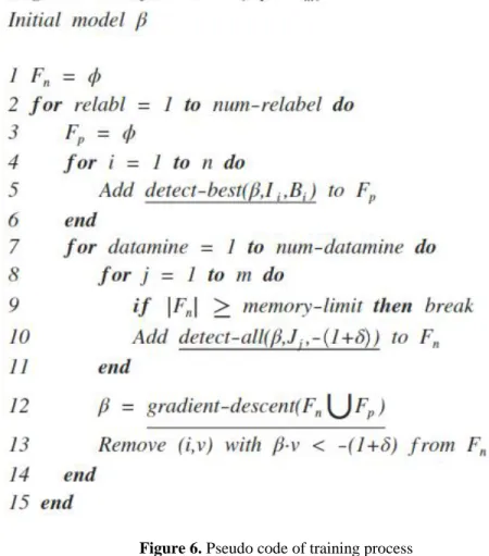
The pseudo code of training process is shown in Figure 6. The first loop from line 2 to 15 implements fixed iteration of coordinate descent. Lines 3 to 5 do the positive example relabeling to optimize 𝑧 while lines 7 to 14 optimize 𝛽. Data-mining algorithm is used to remove hard negative examples for reducing the data size. In every iteration, highest scoring hypothesis is stored in 𝐹_𝑝 while hard negative examples are all collected into 𝐹_𝑛. Then training 𝛽 and remove easy feature vectors from 𝐹_𝑛. The process break when we reach the memory limitation.

Figure 6. Pseudo code of training process

The function 𝑑𝑒𝑡𝑒𝑐𝑡 − 𝑏𝑒𝑠𝑡(𝛽, 𝐼, 𝐵) is used to find the highest scoring hypothesis that specifies a root filter overlap 𝐵 on a large area. The 𝑑𝑒𝑡𝑒𝑐𝑡 − 𝑎𝑙𝑙(𝛽, 𝐼, 𝑡ℎ) is used to find the best hypothesis for a specified root and select ones whose score above 𝑡ℎ. The function

23 4.3.2 Initialization

The coordinate descent algorithm for latent SVM is sensitive to the initialization of model parameters. So here we discuss the procedure of initialization and training.

For training a mixture model with 𝑚 components, we first sort the bounding boxes by their aspect ratio and send them into m groups. Every group has equal size bounding boxes and we train m different root filters, one for each group. We use standard SVM to train these filters on positive dataset 𝑃 with no latent variables. Figure 7 shows two trained models for bicycle.

After we got initialed root filters, we need to combine them together to form a mixture model. This mixture model has no parts information now. Then we train this mixture model following the pseudo code shown above on the whole dataset 𝐷. In this case, the latent information only contains the information of component label and root location.

Next step is to initialize and train part filters. We fix the number of parts for each component as six and we assume parts should be placed on high-energy regions of root. We use a pool of part-shape rectangular to cover these regions and once a region is covered on the root, it is set to be zero. Then we look for a next high-energy region until six parts are chosen. The deformation parameters are initialed as 𝑑 = (0,0, .1, .1).

25

5.0 OCCLUSION HANDLING

In this section, I will mainly introduce an occlusion handling approach based on the mixture deformable part models discussed in section 4.0 and the idea is mainly based on paper [26]. This section includes two parts: introduction of model and implementation of model.

5.1 MODEL

As we discussed before, mixture deformable part model introduced in section 4.0 is consisted of a root filter and a set of part filters. The model can be define as 𝑀 = (𝐹₀, 𝑃₁, … , 𝑃_𝑏, 𝑏) where 𝐹0

is the root filter, 𝑃_𝑖is the model for the 𝑖-th part filter and b is the bias term. Part model is defined as 𝑃𝑖 = (𝐹𝑖, 𝑣𝑖, 𝑑𝑖) where 𝐹𝑖 is the filter for the 𝑖-th part and 𝑑𝑖 is the deformation coefficients, which we will use here to calculate part filter responses.

Given a detection window at position 𝑝 and level 𝑙, the response of root filter is calculated as,

𝑅(𝑝, 𝑙) = 𝐹₀𝑇∙ 𝐺(𝑝, 𝑙) + 𝑏 (5-1) Where 𝐺(𝑝, 𝑙) is the concatenation of features computed on cell level inside the detection box and 𝑏 is the bias term. Since this is a linear operation, we can rewrite the filter response as a summation of responses on cell level. Then the root detector score can be written as,

𝑅₀(𝑝, 𝑙) = ∑𝐶 [(𝐹₀𝑐)𝑇_{∙ 𝐺}𝑐_{(𝑝, 𝑙) + 𝑏}𝑐_]

𝑐=1 = ∑𝐶𝑐=1𝑅0𝑐(𝑝, 𝑙) (5-2) Where 𝐶 is the number of cells and 𝑏 = ∑ 𝑏𝑐. Here we suppose 𝑅_𝑝(𝑝, 𝑙) is the filter response of

𝑝-th part according to the root position and as we know, part filter response is linear on part level. Then the total score of a detection window, which is the summation of root filter response and every part filter response can be calculated as,

𝑅(𝑝, 𝑙) = ∑𝐶 𝑅₀𝑐(𝑙, 𝑝)

𝑐=1 + ∑𝑃𝑝=1𝑅𝑝(𝑝, 𝑙) (5-3) When an object is partially occluded, the occlusion parts may have negative effect to the filter response, which will decrease the detection score. So what we need to do here is to remove the contribution of occluded part to both root filter response and part filter response. So I attach a visibility flag to every cell and part to indicate that whether the cell or part is occluded or not. The visibility flag is a binary variable that 0 indicates occluded and 1 indicates visible. By doing this, we will only aggregate the filter responses of visible cells and parts.

The problem of finding put the values of visibility flags can be treated as a optimization problem on the following score function,

𝑣̂, {𝑣₀ ̂}_𝑝 𝑝=1 𝑃 = 𝑎𝑟𝑔 max 𝑣0,{𝑣𝑝} (∑𝐶_𝑐=1𝑅₀𝑐𝑣₀𝑐+ ∑𝑃_𝑝=1𝑅_𝑝𝑣_𝑝) (5-4) Where 𝑣̂ = [𝑣_{0 0}0, … , 𝑣₀𝐶] and {𝑣̂}_𝑝 𝑝=1 𝑃

are the visibility flags for cells of root and parts. Here we omit the parameter 𝑝 and 𝑙 for simplicity and the function only focus on one detection window. The maximization result of the score function above will simply set visibility flag 0 for cells and parts whose filter response below zero and 1 for others. But occluded regions are not likely to be distributed evenly on the object. There some occlusion “rules” we need to follow.

First of all, the object is usually occluded by another object, which means occlusion likely to occur on a continuous region. What’s more, the root cells and parts that are overlapped

27

should have the same visibility flag value. To account these spatial relations, we can add two penalty terms, cell-to-cell consistency and part-to-part consistency, to the score function. Then the function takes the following form,

𝑅_𝑜𝑐𝑐 = max 𝑣0,{𝑣𝑝}_𝑝=1 𝑃 ∑ 𝑅0 𝑐_𝑣 0𝑐 + ∑ 𝑅𝑝𝑣𝑝 𝑃 𝑝=1 𝐶 𝑐=1 −𝛾 ∑ |𝑣₀𝑐𝑖_{− 𝑣} 0 𝑐𝑗 | − 𝑐𝑖~𝑐𝑗 𝛾 ∑ |𝑣0 𝑐𝑖_{− 𝑣} 0 𝑝𝑗 | 𝑐𝑖~𝑝𝑗 (5-5)

Where 𝑐_𝑖 and 𝑐_𝑗 are adjacent cells, 𝑐_𝑖 and 𝑝_𝑗 are overlapped cell and part, 𝛾 is the regularization parameter.

Since the dataset I will use to test the model is a pedestrian detection dataset, in street scene, lower part of the pedestrian are more likely to be occluded than the upper part. So here I also introduce two penalty terms to control the position of the occlusion region. Then the score function can be written as,

𝑅_𝑜𝑐𝑐 = max 𝑣0,{𝑣𝑝}_𝑝=1 𝑃 ∑ [𝑅0 𝑐_𝑣 0𝑐− 𝛼𝜆0𝑐(1 − 𝑣0𝑐)] + ∑ [𝑅𝑝𝑣𝑝 𝑃 𝑝=1 𝐶 𝑐=1 − 𝛽𝜆_𝑝(1 − 𝑣_𝑝)] −𝛾 ∑ |𝑣₀𝑐𝑖_{− 𝑣} 0 𝑐𝑗 | − 𝑐𝑖~𝑐𝑗 𝛾 ∑ |𝑣0 𝑐𝑖_{− 𝑣} 0 𝑝𝑗 | 𝑐𝑖~𝑝𝑗 (5-6)

Where 𝜆₀𝑐 and 𝜆𝑝 are penalties when visibility flags of cells and parts are set occluded, 𝛼 and 𝛽 are weights of the penalty term. The value of 𝜆₀𝑐 and 𝜆_𝑝 should be proportional to the height from the bottom of image to the cell or part. When the cell or part is in upper area of the image, the penalty of setting their visibility flags to 0 should be large. It can be calculated follow the sigmoid function as,

𝜆 =1 2[ 1 1+𝑒−𝜏(ℎ−ℎ0 2⁄ )+ 1 2] (5-7) where ℎ is the height of cell or part from the bottom of image and 𝜏 controls the step size.

5.2 IMPLEMENTATION

There are a large number of detection windows in an image, so computing visibility flags for all these windows will be very time-consuming. So here we run the DPM detector on an image first and pick top 10% from all detection windows as our candidates. Then we attach visibility flags to these candidates and here we introduce Alternation Direction Method of Multipliers (ADMM) [16] to speed up the optimization process.

The function (5-6) can be rewritten as the following ADMM form,

𝑚𝑖𝑛𝑖𝑚𝑖𝑧𝑒 − 𝜔𝑇𝑞 + 𝜆‖𝑧₁‖₁+ 𝐽_[0,1](𝑧₂)

𝑠𝑢𝑏𝑗𝑒𝑐𝑡 𝑡𝑜 𝐷𝑞 = 𝑧₁, 𝑞 = 𝑧₂, 𝑞 ∈ [0,1]𝐶+𝑃 _(5-8) where q = [v₀0, … , v₀C, v₁, … , v_p]𝑇 is the concatenation of visibility flags of cells and parts, 𝜔 = [(𝑅₀0+ 𝛼𝜆₀0), … , (𝑅₀𝐶_{+ 𝛼𝜆}

0 𝐶_{), (𝑅}

1+ 𝛽𝜆1), … , (𝑅𝑝+ 𝛽𝜆𝑝)] 𝑇

is the stack of filter responses and a penalty term parameter. D here is a (𝐶 + 𝑃) × (𝐶 + 𝑃) differentiation matrix for cell-to-cell consistency and cell-to-part consistency penalty terms. 𝐽_[0,1](𝑧₂) is an indicator function.

𝐽_[0,1](𝑧₂) = 0 when 𝑧₂ between 0 to 1, otherwise 𝐽_[0,1](𝑧₂) = +∞. Then we can get the augment

Lagrangian function as following,

𝐿(𝜔, 𝑧1, 𝑧2, 𝑢1, 𝑢2) = −𝜔𝑇𝑞 + 𝜆‖𝑧1‖1+ 𝐽[0,1](𝑧2) +𝜌1 2 ‖𝐷𝑞 − 𝑧1+ 𝑢1‖2 2 +𝜌2 2 ‖𝑞 − 𝑧2+ 𝑢2‖2 2 _(5-9) where 𝜌1 > 0, 𝜌2 > 0 are penalty terms. Here tried different values for parameters (𝜆, 𝜌1, 𝜌2) and find best value set. This will be discussed in detail in next section.

29

6.0 EXPERIMENTS

6.1 DETECTION OF FULLY VISIBLE OBJECTS

The Deformation Part Model is tested on PASCAL VOC 2006 [20], 2007 [18] and 2008 [19]. These are very difficult dataset for object detection challenge. Each dataset has thousands of images with one or more different objects on them. Every object is has a ground-truth bounding box. In the test process, our goal is to predict the bounding box for a given class object. Since the system returns several high-scoring bounding box candidates, so we need to set a threshold to pick out better results from these candidates. A prediction of bounding box can be treated as correct when it overlap the ground-truth bounding box over 50%. Sometimes the system with return several bounding boxes that overlap together, in this case, we will only consider one of them is correct, and the others are false.

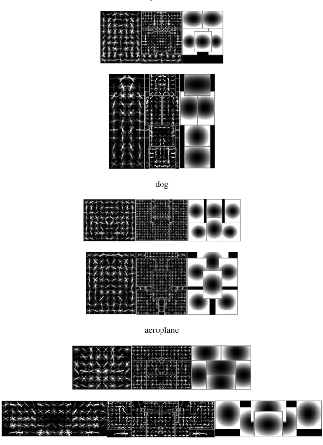
Every model consists of two components. Figure 8 shows some mixture models trained on PASCAL 2007 set. Figure 9 shows some detection results we get by using these models.

person

dog

aeroplane

31

6.2 DETECTION OF PARTIALLY OCCLUDED OBJECTS

The test dataset for partially occluded objects we choose here is Daimler Multi-Cue Occluded Pedestrian Classification benchmark [13], which contains a large variety set of partially occluded pedestrians with cars or other non-pedestrian objects as occluders. Note that the occlusion handling model here in this paper is not able to deal with pedestrian-to-pedestrian occlusion. That’s why the most other relative datasets like ETH [23] and Caltech Pedestrian Detection Benchmark [24] cannot be used here.

The training and testing part of the dataset contain labeled pedestrians and non-pedestrians bounding boxes. All the images of the dataset are taken from a vehicle-mounted camera in an urban environment. Positive samples are manually labeled while the negative samples are based on pre-processed with relaxed threshold setting. Besides formal intensity image, the dataset also contains dense stereo samples and dense optical flow samples. There are totally 80,000 training samples as well as 50,000 testing samples. Each sample has a 96*48 resolution with a border of 12 pixels around the pedestrian. Intensity samples are the only samples used in my test.

In practice, the minimization problem of function (5-9) has parameters such as 𝜆, 𝜌₁,

𝜌₂, 𝛼, to be set. But the Daimler dataset only provides test set for occluded pedestrian detection. There is not enough data used to train these parameters. So here I just try a range of values of every parameter and find the parameter set that produces highest detection score.

33

35

Figure 10, Figure 11 and Figure 12 shows the detection accuracy value according to different parameter set. To reduce the search space, I assume that 𝜌₁ = 𝜌₁. When the bounding box returned by the system overlaps the ground-truth bounding box over 50%, then we treat the detection result as accurate. Otherwise, we treat it as false detection. The highest scoring parameter set we get is (𝜆 = 1.4, 𝜌₁ = 1, 𝜌₂ = 1, 𝛼 = 1.4).

Even though only the cell information and part information alone cannot determine whether a region is occluded or not, this information combined with penalty term will provide a relatively robust model handing occlusion problems. Figure 13 shows some detection results on the Daimler dataset.

I compare the occlusion handling model with mixture deformation part model by testing both of them on the partially occluded and non-occluded pedestrian datasets. And the test result is shown in Table 1. From the table we can see clearly that the accuracy rate of partially occluded object detection is significantly improved compared with DPM.

Table 1. Comparison of occlusion handling model and DPM

Partially occluded Non-occluded

Occlusion Handling 0.9717 0.9884

37

Figure 13. Some detection results:

Original input image (left). Cell occlusion detection (middle). Regions covered with read lines are occluded. Part occlusion detection (right). Parts with red bounding box lines are occluded.

7.0 CONCLUSION

In this paper, we introduce a state-of-art object detection model, mixture Deformable Part Model, and based on this model, we introduce an occlusion handling approach. We attach visibility flags to every root cells and parts and by doing convex function optimization, then we get tall he flag values. We do test on the Daimler Multi-Cue Occluded Pedestrian Classification benchmark and the experiments show that the accuracy rate of partially occluded object detection improved significantly. But there is still storage of this model: it cannot deal with pedestrian-to-pedestrian occlusion. I will do more future research on it.

39

BIBLIOGRAPHY

[1] Felzenszwalb, Pedro F., et al. "Object detection with discriminatively trained part-based models." Pattern Analysis and Machine Intelligence, IEEE Transactions on 32.9 (2010): 1627-1645.

[2] Dalal, Navneet, and Bill Triggs. "Histograms of oriented gradients for human detection." Computer Vision and Pattern Recognition, 2005. CVPR 2005. IEEE Computer

Society Conference on. Vol. 1. IEEE, 2005.

[3] Dollar, Piotr, et al. "Pedestrian detection: An evaluation of the state of the art."Pattern

Analysis and Machine Intelligence, IEEE Transactions on 34.4 (2012): 743-761.

[4] Wang, Xiaoyu, Tony X. Han, and Shuicheng Yan. "An HOG-LBP human detector with partial occlusion handling." Computer Vision, 2009 IEEE 12th International Conference on. IEEE, 2009.

[5] Vedaldi, Andrea, and Andrew Zisserman. "Structured output regression for detection with partial truncation." Advances in neural information processing systems. 2009.

[6] Gao, Tianshi, Benjamin Packer, and Daphne Koller. "A segmentation-aware object detection model with occlusion handling." Computer Vision and Pattern Recognition

(CVPR), 2011 IEEE Conference on. IEEE, 2011.

[7] Ouyang, Wanli, and Xiaogang Wang. "A discriminative deep model for pedestrian detection with occlusion handling." Computer Vision and Pattern Recognition (CVPR),

2012 IEEE Conference on. IEEE, 2012.

[8] Niknejad, Hossein Tehrani, et al. "Occlusion handling using discriminative model of trained part templates and conditional random field." Intelligent Vehicles Symposium (IV), 2013 IEEE. IEEE, 2013.

[9] Azizpour, Hossein, and Ivan Laptev. "Object detection using strongly-supervised deformable part models." Computer Vision–ECCV 2012. Springer Berlin Heidelberg, 2012. 836-849.

[10] Girshick, Ross B., Pedro F. Felzenszwalb, and David A. Mcallester. "Object detection with grammar models." Advances in Neural Information Processing Systems. 2011.

[11] Yu, Xiang, et al. "Consensus of regression for occlusion-robust facial feature localization." Computer Vision–ECCV 2014. Springer International Publishing, 2014. 105-118.

[12] Ghiasi, Golnaz, and Charless Fowlkes. "Occlusion coherence: Localizing occluded faces with a hierarchical deformable part model." Proceedings of the IEEE Conference on

Computer Vision and Pattern Recognition. 2014.

[13] Baumgartner, Tobias, Dennis Mitzel, and Bastian Leibe. "Tracking people and their objects." Proceedings of the IEEE Conference on Computer Vision and Pattern Recognition. 2013.

[14] Enzweiler, Markus, et al. "Multi-cue pedestrian classification with partial occlusion handling." Computer vision and pattern recognition (CVPR), 2010 IEEE Conference on. IEEE, 2010.

[15] Mathias, Markus, et al. "Handling occlusions with franken-classifiers."Proceedings of the

IEEE International Conference on Computer Vision. 2013.

[16] Tang, Siyu, Mykhaylo Andriluka, and Bernt Schiele. "Detection and tracking of occluded people." International Journal of Computer Vision 110.1 (2014): 58-69.

[17] Wahlberg, Bo, et al. "An ADMM algorithm for a class of total variation regularized estimation problems." arXiv preprint arXiv:1203.1828 (2012).

[18] Andrews, Stuart, Ioannis Tsochantaridis, and Thomas Hofmann. "Support vector machines for multiple-instance learning." Advances in neural information processing systems. 2002. [19] Everingham, Mark, et al. "The pascal visual object classes challenge (voc2007) results."

[Online] Available: http://www.pascal-network.org/challenges/VOC/voc2007/

[20] Everingham, Mark, et al. "The pascal visual object classes challenge (voc2008) results." [Online] Available: http://www.pascal-network.org/challenges/VOC/voc2008/

[21] Everingham, Mark, et al. "The pascal visual object classes challenge (voc2006) results." [Online] Available: http://www.pascal-network.org/challenges/VOC/voc2006/

[22] Boyd, Stephen, et al. "Distributed optimization and statistical learning via the alternating direction method of multipliers." Foundations and Trends® in Machine Learning 3.1 (2011): 1-122.

41

[23] Dollár, Piotr, et al. "Pedestrian detection: A benchmark." Computer Vision and Pattern

Recognition, 2009. CVPR 2009. IEEE Conference on. IEEE, 2009.

[24] Ess, Andreas, Bastian Leibe, and Luc Van Gool. "Depth and appearance for mobile scene analysis." Computer Vision, 2007. ICCV 2007. IEEE 11th International Conference on. IEEE, 2007.

[25] Tang, Siyu, Mykhaylo Andriluka, and Bernt Schiele. "Detection and tracking of occluded people." International Journal of Computer Vision 110.1 (2014): 58-69.

[26] Felzenszwalb, Pedro, and Daniel Huttenlocher. Distance transforms of sampled functions. Cornell University, 2004.

[27] Chan, Kai Chi, Alper Ayvaci, and Bernd Heisele. "Partially occluded object detection by finding the visible features and parts." Image Processing (ICIP), 2015 IEEE International