Graph Kernels and Applications in Bioinformatics

(1)

DigitalCommons@USU

All Graduate Theses and Dissertations Graduate Studies

5-2011

Graph Kernels and Applications in Bioinformatics

Marco Alvarez Vega

Utah State University

Follow this and additional works at: https://digitalcommons.usu.edu/etd Part of the Computer Sciences Commons

Recommended Citation Recommended Citation

Alvarez Vega, Marco, "Graph Kernels and Applications in Bioinformatics" (2011). All Graduate Theses and Dissertations. 1185.

https://digitalcommons.usu.edu/etd/1185 This Dissertation is brought to you for free and open access by the Graduate Studies at

DigitalCommons@USU. It has been accepted for inclusion in All Graduate Theses and Dissertations by an authorized administrator of DigitalCommons@USU. For more information, please contact

(2)

by

Marco Alvarez Vega

A dissertation submitted in partial fulfillment of the requirements for the degree

of

DOCTOR OF PHILOSOPHY in

Computer Science

Approved:

Dr. Xiaojun Qi Dr. Changhui Yan

Major Professor Committee Member

Dr. Minghui Jiang Dr. Adele Cutler

Committee Member Committee Member

Dr. Vicki Allan Dr. Mark R. McLellan

Committee Member Vice President for Research and

Dean of the School of Graduate Studies

UTAH STATE UNIVERSITY Logan, Utah

(3)

Abstract

Graph Kernels and Applications in Bioinformatics

by

Marco Alvarez Vega, Doctor of Philosophy Utah State University, 2011

Major Professor: Dr. Xiaojun Qi Department: Computer Science

In recent years, machine learning has emerged as an important discipline. However, despite the popularity of machine learning techniques, data in the form of discrete structures are not fully exploited. For example, when data appear as graphs, the common choice is the transformation of such structures into feature vectors. This procedure, though convenient, does not always effectively capture topological relationships inherent to the data; therefore, the power of the learning process may be insufficient. In this context, the use of kernel functions for graphs arises as an attractive way to deal with such structured objects.

On the other hand, several entities in computational biology applications, such as gene products or proteins, may be naturally represented by graphs. Hence, the demanding need for algorithms that can deal with structured data poses the question of whether the use of kernels for graphs can outperform existing methods to solve specific computational biology problems. In this dissertation, we address the challenges involved in solving two specific problems in computational biology, in which the data are represented by graphs.

First, we propose a novel approach for protein function prediction by modeling pro-teins as graphs. For each of the vertices in a protein graph, we propose the calculation of evolutionary profiles, which are derived from multiple sequence alignments from the amino acid residues within each vertex. We then use a shortest path graph kernel in conjunction

(4)

with a support vector machine to predict protein function. We evaluate our approach under two instances of protein function prediction, namely, the discrimination of proteins as en-zymes, and the recognition of DNA binding proteins. In both cases, our proposed approach achieves better prediction performance than existing methods.

Second, we propose two novel semantic similarity measures for proteins based on the gene ontology. The first measure directly works on the gene ontology by combining the pairwise semantic similarity scores between sets of annotating terms for a pair of input proteins. The second measure estimates protein semantic similarity using a shortest path graph kernel to take advantage of the rich semantic knowledge contained within ontologies. Our comparison with other methods shows that our proposed semantic similarity measures are highly competitive and the latter one outperforms state-of-the-art methods. Further-more, our two methods are intrinsic to the gene ontology, in the sense that they do not rely on external sources to calculate similarities.

(5)

Public Abstract

Graph Kernels and Applications in Bioinformatics

Nowadays, machine learning techniques are widely used for extracting knowledge from data in a large number of bioinformatics problems. It turns out that in many of such problems, data observations can be naturally represented by discrete structures such as graphs, networks, trees, or sequences. For example, a protein can be seen as a cloud of interconnected atoms lying on a 3-dimensional space. The focus of this dissertation is on the development and application of machine learning techniques to bioinformatics problems wherein the data can be represented by graphs. In particular, we focus our attention on proteins, which are essential elements in the life process. The study of their underlying structure and function is one of the most important subjects in bioinformatics. As proteins can be naturally represented by graphs, we consider the use of kernel functions that can directly deal with data observations in the form of graphs. Kernel functions are the basic building block for a powerful family of machine learning algorithms called kernel methods. Concretely, we propose a novel approach for predicting the function of proteins. We model proteins as graphs, and we predict function using support vector machines and graph kernels. We evaluate our approach under two types of function prediction, the discrimina-tion of proteins as enzymes or not, and the recognidiscrimina-tion of DNA binding proteins. In both cases, the resulting performance is higher than existing methods.

In addition, given the establishment of ontologies as a popular topic in biomedical research, we propose two novel semantic similarity measures between pairs of proteins. First, we introduce a novel semantic similarity method between pairs of gene ontology terms. Second, we propose an instance of the shortest path graph kernel for calculating the semantic similarity between proteins. This latter approach, when compared with state-of-the-art methods, yields an improved performance.

(6)

(7)

Acknowledgments

Many people have contributed in different ways to the work contained in this disser-tation. I sincerely thank professors Xiaojun Qi, Changhui Yan, and Seungjin Lim. They have provided the required resources and supervision along the completion of this work. I am also greatly indebted to Dr. Xiaojun Qi for her encouragement and words of wisdom.

I would like to express my gratitude and appreciation to Dr. Adele Cutler for her valuable advice and motivation that have led me to pursue interesting research topics in machine learning. I am grateful to my committee members for having followed my work. I would also like to thank Myra Cook for her assistance with refining this dissertation.

I would like to acknowledge the Center for High Performance Computing at Utah State University for enabling the development of computationally intensive research activities. Thanks to their resources, I was able to reduce the running time of each experiment from several days to hours.

There are many individuals who have contributed to my academic career since I started my undergraduate studies. I am always grateful to all my former professors, especially Dr. Andre de Carvalho at the University of S˜ao Paulo and Dr. Nalvo de Almeida Jr at the Federal University of Mato Grosso do Sul for their continuous support. I should also acknowledge former colleagues at the Dom Bosco Catholic University, Dr. Milton Romero and Dr. Hemerson Pistori, for their encouragement, friendship, and recommendations for accomplishing my goals.

Finally, I want to express my love to my family and friends in Brazil, Peru, and Logan. My parents, sisters, “T´ıo Mario”, “T´ıas Vicky and Ruth”, Miguel and many other relatives and friends have played a huge role when adversity came around during this journey.

(8)

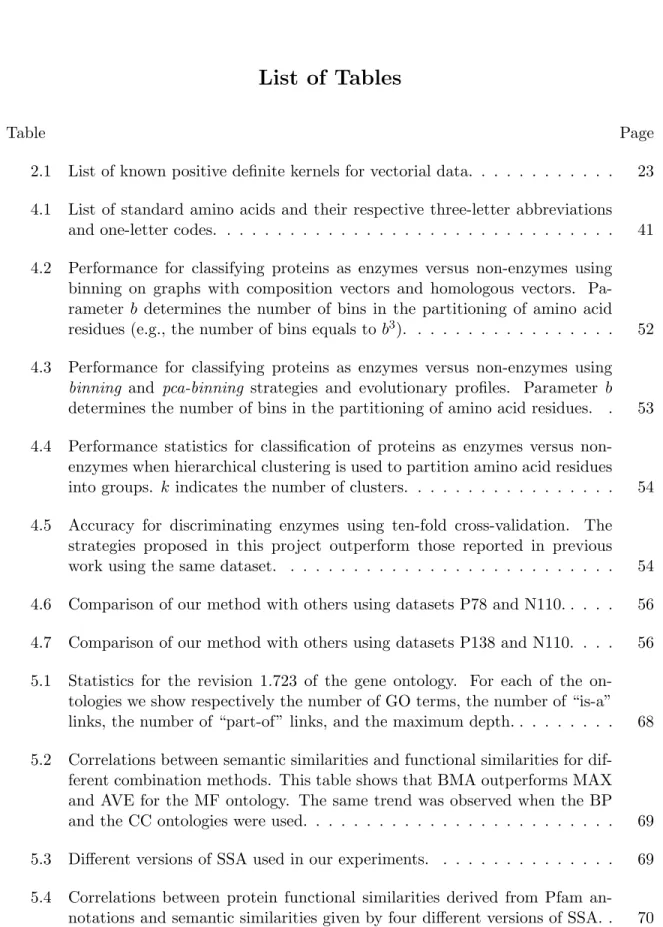
List of Tables

Table Page

2.1 List of known positive definite kernels for vectorial data. . . 23 4.1 List of standard amino acids and their respective three-letter abbreviations

and one-letter codes. . . 41 4.2 Performance for classifying proteins as enzymes versus non-enzymes using

binning on graphs with composition vectors and homologous vectors. Pa-rameter b determines the number of bins in the partitioning of amino acid residues (e.g., the number of bins equals to b3_{). . . .} ₅₂ 4.3 Performance for classifying proteins as enzymes versus non-enzymes using

binning and pca-binning strategies and evolutionary profiles. Parameter b determines the number of bins in the partitioning of amino acid residues. . 53 4.4 Performance statistics for classification of proteins as enzymes versus

non-enzymes when hierarchical clustering is used to partition amino acid residues into groups. kindicates the number of clusters. . . 54 4.5 Accuracy for discriminating enzymes using ten-fold cross-validation. The

strategies proposed in this project outperform those reported in previous work using the same dataset. . . 54 4.6 Comparison of our method with others using datasets P78 and N110. . . 56 4.7 Comparison of our method with others using datasets P138 and N110. . . . 56 5.1 Statistics for the revision 1.723 of the gene ontology. For each of the

on-tologies we show respectively the number of GO terms, the number of “is-a” links, the number of “part-of” links, and the maximum depth. . . 68 5.2 Correlations between semantic similarities and functional similarities for

dif-ferent combination methods. This table shows that BMA outperforms MAX and AVE for the MF ontology. The same trend was observed when the BP and the CC ontologies were used. . . 69 5.3 Different versions of SSA used in our experiments. . . 69 5.4 Correlations between protein functional similarities derived from Pfam

(11)

5.5 Resolution values obtained for sequence similarity and correlation values ob-tained for EC class and Pfam similarities for SSAv3 and other methods im-plemented in CESSM. . . 73 5.6 Resolution values for simspgk and other methods implemented in CESSM.

Note also that simspgk yields higher resolution than SSA, described in Sec-tion 5.2. . . 77 5.7 Correlation values between semantic similarities and functional similarities

derived from EC classification. . . 77 5.8 Correlation values between semantic similarities and functional similarities

(12)

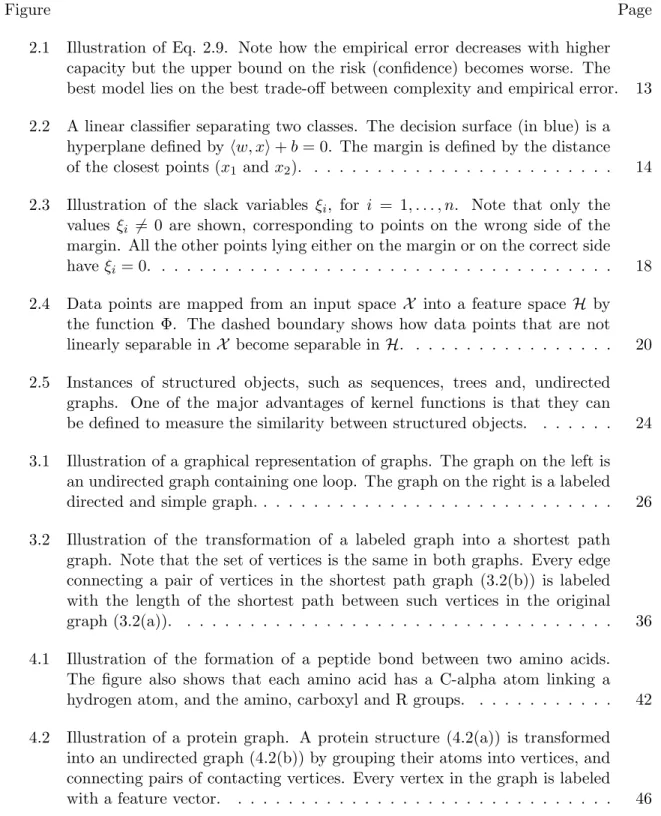
List of Figures

Figure Page

2.1 Illustration of Eq. 2.9. Note how the empirical error decreases with higher capacity but the upper bound on the risk (confidence) becomes worse. The best model lies on the best trade-off between complexity and empirical error. 13 2.2 A linear classifier separating two classes. The decision surface (in blue) is a

hyperplane defined by_hw, x_i+b= 0. The margin is defined by the distance of the closest points (x1 and x2). . . 14 2.3 Illustration of the slack variables ξi, for i = 1, . . . , n. Note that only the

values ξi 6= 0 are shown, corresponding to points on the wrong side of the margin. All the other points lying either on the margin or on the correct side have ξi = 0. . . 18 2.4 Data points are mapped from an input space _X into a feature space _H by

the function Φ. The dashed boundary shows how data points that are not linearly separable in _X become separable in _H. . . 20 2.5 Instances of structured objects, such as sequences, trees and, undirected

graphs. One of the major advantages of kernel functions is that they can be defined to measure the similarity between structured objects. . . 24 3.1 Illustration of a graphical representation of graphs. The graph on the left is

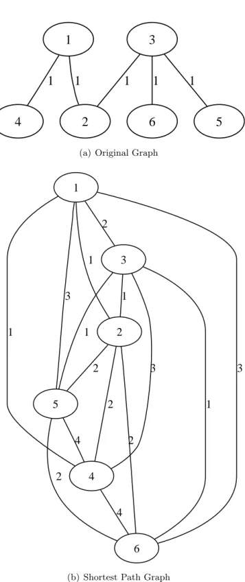
an undirected graph containing one loop. The graph on the right is a labeled directed and simple graph. . . 26 3.2 Illustration of the transformation of a labeled graph into a shortest path

graph. Note that the set of vertices is the same in both graphs. Every edge connecting a pair of vertices in the shortest path graph (3.2(b)) is labeled with the length of the shortest path between such vertices in the original graph (3.2(a)). . . 36 4.1 Illustration of the formation of a peptide bond between two amino acids.

The figure also shows that each amino acid has a C-alpha atom linking a hydrogen atom, and the amino, carboxyl and R groups. . . 42 4.2 Illustration of a protein graph. A protein structure (4.2(a)) is transformed

into an undirected graph (4.2(b)) by grouping their atoms into vertices, and connecting pairs of contacting vertices. Every vertex in the graph is labeled with a feature vector. . . 46

(13)

4.3 Binning applied to a set of 2-dimensional points with parameter b= 3 . In this example, the graph will contain only 7 vertices because two bins do not contain any points. Bear in mind that 2-dimensional points are used only for illustration purposes. In our work, the points lie on a 3-dimensional space. . 47 4.4 PCA-binning applied to the same set of points as in Figure 4.3. The

calcula-tion of the principal components is shown in Figure 4.4(a) and the applicacalcula-tion of simple binning to the transformed points is illustrated in Figure 4.4(b). Note how the points tend to be distributed in all the bins. A 2-dimensional space is used for illustration purposes. C-alpha atoms are in fact 3-dimensional. 48 4.5 Clustering applied to a set of 12 amino acid residues. For this illustration

four clusters, shown in different colors within the four rounded rectangles, are found by the HAC algorithm. Note how HAC chooses neighboring points to form final clusters. Non-empty clusters become vertices in the graph. . . 48 5.1 Graph including all terms annotating protein P17252 (protein kinase C

al-pha type) from the cellular component ontology. All the ancestors of the annotating terms are also included in the graph. . . 75

(14)

Chapter 1 Introduction

In many real world problems, data observations occur naturally as complex structures, which in turn can be represented by powerful formalisms such as graphs. Generally speaking, a graph is defined as a collection of vertices or nodes where pairs of vertices are connected by edges. Graphs are increasingly being used to model structured data objects in more and more domains. For example, in social science, social networks are represented as finite graphs of ties between social actors [1]. In natural language processing, graphs are used to encode the meaning and structure of texts [2]. In chemoinformatics, graphs are the fundamental way for representing chemical compounds [3]. In bioinformatics, graphs and sequences are also used to represent the information contained in important bodies such as biomolecules, DNA, RNA, and proteins [4]. Note that from a computational perspective, sequences are in fact a special case of graphs.

Particularly in bioinformatics, recent scientific and technological advances have con-tributed to the production of enormous amounts of structured data, which are available in private and public repositories. This context has brought the attention of machine learning and data mining researchers, who are increasingly focusing on the study of patterns existing in such structures [5]. One case of great interest and importance is the study of protein function.

Proteins are essential macromolecules responsible for performing numerous functions in living cells. Understanding their function is crucial for promoting the advancement of knowledge in biology and life sciences in general. Each protein within the body has a specific function. For example, inside a cell we find a special type of protein, the enzyme, which is known to increase the rate of chemical reactions.

(15)

in distinct ways. Based on the sequence of amino acid residues on protein chains, we can represent proteins as sequences of letters with each letter representing one amino acid residue. Based on the structure of a protein, i.e., the spatial coordinates of each of the atoms constituting a protein, we can represent proteins as point clouds in a 3-dimensional space. Several structural genomics projects, whose goal is to determine the 3-dimensional structure of proteins, have been producing a vast number of protein structures. Furthermore, due to the difficulties involved in the experimental characterization of protein function, these projects have been generating a large number of proteins with little or unknown functional information [6]. Consequently, effective and high-throughput computational approaches are needed for addressing the problem of predicting the unknown function of proteins. In this dissertation, we investigate graph models for proteins that can effectively represent their rich structural information. We propose the use of such models in conjunction with graph kernels and support vector machines for predicting protein function in two specific problems: the prediction of proteins as enzymes and the prediction of proteins as DNA binding proteins.

In machine learning, kernel methods such as the widely used support vector machine, are a class of very powerful algorithms for pattern analysis and prediction [7–9]. A crucial point in kernel methods is that they depend on the data only through the calculation of kernel functions. Therefore, algorithms of the family of kernel methods are based upon the use of kernel functions (or simply “kernels”), which can be thought of as similarity measures for pairs of objects. In statistical learning theory, a kernel function K(x, y) for a pair of data observationsxandy is a formalism used to extend linear methods to work in a higher dimensional space where nonlinearities in the data can be detected. Several kernel functions are available in the literature, the most popular of which assume that the observations are feature vectors, i.e., arrays of numeric values. A list of some kernels defined to work on feature vectors include: linear, polynomial, gaussian, exponential, and laplacian kernels [9]. It turns out that we can also define kernel functions for pairs of discrete structures. More specifically, we can define kernel functions for graph models of proteins. Thus, the

(16)

entire family of kernel methods is available for building prediction models by directly pro-cessing datasets of graphs. This appears as an elegant and effective way for solving protein function prediction problems. Among all recent developments, graph kernels based on shortest paths [10], are a remarkable class of kernel functions. They are able to compare graphs at acceptable polynomial time. Contrary to most existing graph kernels, shortest path graph kernels can deal with graphs with continuous feature vectors at their nodes. In our approach, shortest path graph kernels are used in conjunction with support vector machines to train models for predicting protein function.

On the other hand, a totally different way to characterize proteins is the use of onto-logical annotations, that is, by labeling proteins with multiple terms defined in a related ontology. Ontologies are a popular topic in various fields of computer science [11]. They are primarily used to represent the knowledge within a domain, by means of a hierarchical structure of concepts connected by relationships between them. This formal specification permits the description of entities within the investigated domain, and eventually, the use of computational methods for reasoning about such entities. In bioinformatics, the gene ontology [12] is a major initiative to systematically organize biological knowledge across species and databases.

The gene ontology provides a controlled vocabulary of terms used to characterize gene products, either RNA or proteins, in terms of their associated biological processes, cellular components, and molecular functions. The vocabulary of terms is organized as a directed acyclic graph, where each term has defined relationships to one or more other terms. Given the vocabulary, proteins can be annotated with terms to describe their characteristics. A rich repository of protein annotations by gene ontology terms is produced by the GOA project [13] held at the European Bioinformatics Institute, which provides high-quality an-notations to proteins in the UniProt KnowledgeBase. The extensive coverage of biological knowledge in the gene ontology in conjunction with the increasing number of protein anno-tations deposited in their respective databases, make these resources valuable components for the analysis of proteins.

(17)

For instance, proteins can be compared based on the semantic similarity between their respective annotating terms. The term semantic similarity is a measure for the likeness of the meaning of the involved terms. Therefore, protein semantic similarity can be derived by analyzing their respective annotation sets and the semantic relationships of such terms in the gene ontology. In this dissertation, we also propose graph models for proteins based on their respective annotating terms and relationships in the gene ontology. Given such models, we propose two novel ways to estimate the semantic similarity between pairs of proteins. The estimation of semantic similarity between a pair of proteins is a basic building block that can be incorporated in the study of protein function.

1.1 Contributions

In view of the abundance of structured data in bioinformatics, specifically, data pro-vided by databases of protein structures, the gene ontology, and databases of annotated proteins, we focus on the study and proposal of computational approaches that can take ad-vantage of the rich amount of information contained in proteins, when they are represented as structured objects. To this end, we consider two distinct problems in bioinformatics, namely, protein function prediction and protein semantic similarity.

1.1.1 Protein Function Prediction

We address the problem of protein function prediction by proposing a novel approach for modeling proteins as graphs. For a given protein, a graph model is created by combining information derived from the protein sequence and structure. We apply our approach to two separate binary classification problems, namely, the discrimination of proteins as enzymes, and the discrimination of proteins as DNA-binding proteins. In both cases, graph kernels and support vector machines are used to train the binary classifiers. In summary, our contributions for protein function prediction are highlighted below:

• We propose novel graph models for proteins. We analyze the 3-dimensional protein structure in order to create a protein graph, wherein the vertices represent groups

(18)

of neighboring amino acid residues, and edges connect pairs of vertices that are in contact, i.e., vertices whose their closest atoms are under a minimum distance defined as 5 ˚A;

• We propose the calculation of evolutionary profiles for each of the vertices in a protein graph. These profiles are derived from multiple sequence alignments for the amino acid residues residing within the vertex. The motivation behind this idea is to characterize those regions in the protein structure that seem to be more conserved over time;

• We propose to apply our graph models to datasets of protein structures, so that, shortest path graph kernels can be used in conjunction with the support vector ma-chine algorithm for binary classification in two distinct protein function problems. We show that our proposed approach outperforms other state-of-the-art methods in both problems, the discrimination of enzymes and the recognition of DNA binding proteins. The publications derived from this work are [14, 15].

1.1.2 Protein Semantic Similarity

We also focus our attention on the problem of calculating the semantic similarity be-tween proteins. We propose two novel methods to estimate protein semantic similarity. In both methods, the similarity score for a pair of proteins is derived from their respective annotations from the gene ontology. The hierarchical structure of the gene ontology al-lows us to model proteins as graphs. For example, for a given protein, a graph model can be created by extracting a subgraph from the gene ontology, such that it contains all the terms (vertices) annotating the protein, along with their respective ancestors in the ontol-ogy. This subgraph also includes the relationships (edges) existing in the gene ontology between each pair of vertices. Once gene ontology terms and their relationships provide very valuable semantic knowledge that can be used for estimating functional similarities between proteins, we present our methods under the common denomination of protein se-mantic similarity. Our contributions for estimating the sese-mantic similarity between pairs of proteins are highlighted below:

(19)

• We propose a semantic similarity method that can work directly on the gene ontol-ogy. For a pair of input proteins, their similarity is calculated by combining pairwise semantic similarity scores between their respective annotating terms. To this end, we estimate the semantic similarity between a pair of gene ontology terms, by taking into account the length of the shortest path between them, the depth of their nearest common ancestor, and the semantic similarity between the definitions accompanying both terms. To the best of our knowledge, this is the first attempt to use similar-ities between definitions of terms from the gene ontology to compute the semantic similarity. The publications directly associated with this method are [16–18];

• We propose a novel method for estimating protein semantic similarity. We estimate similarity by representing two input proteins as induced subgraphs from the gene ontology, and then applying an instance of the shortest path graph kernel. By using this kernel function, machine learning methods based on kernels can take advantage of the rich semantic knowledge contained within ontologies and be directly applied to datasets of proteins. The publication derived from this method is [19];

• We introduce the above two novel methods with the advantage that they are intrinsic to the gene ontology, in the sense that they do not rely on external sources to cal-culate similarities. Most of existing methods include scores calcal-culated from external annotation databases; therefore, they are likely to be biased by proteins that are stud-ied more intensively [20]. In a comprehensive evaluation using a benchmark dataset, both of our proposed methods compare favorably with other existing methods. Our approaches provide an alternative route, with comparable performance, to methods that use external resources.

1.2 Organization of This Dissertation

The remainder of this dissertation is organized as follows. In Chapter 2, we introduce basic concepts and terminology related to statistical learning theory and kernel methods.

(20)

Such elements are essential for understanding kernel functions for the graph domain. Chap-ter 3 reviews state-of-the-art kernels for graphs, which are the major ingredients for solving two computational biology problems: protein function prediction and protein semantic sim-ilarity. Chapter 4 describes our proposed graph models for protein structures and their evaluation under two different function prediction problems: the discrimination of proteins as enzymes and the prediction of DNA binding proteins. Chapter 5 reviews the problem of protein semantic similarity and describes our two proposed algorithms: SSA and the short-est path graph kernel, which are accompanied by their respective evaluation and comparison with state-of-the-art methods. Finally, Chapter 6 summarizes our contributions with their respective publications. It also suggests directions for future work.

(21)

Chapter 2 Statistical Learning and Kernel Methods

This chapter introduces the basic foundations of learning theory and kernel methods. They provide the formalisms required to explore and understand kernel methods in the graph domain and their application to computational biology problems.

The chapter starts by introducing the basic concepts and definitions supporting sta-tistical learning theory. Then the formulation of support vector machines is described in detail in conjunction with the connection existing between risk minimization principles and learning with linear classifiers. Finally, kernels are presented as an attractive way to extend linear classifiers to nonlinear spaces.

As the protein function prediction problems described in this dissertation are classi-fication problems involving only two classes, when possible, the examples and settings for the concepts described in this chapter are primarily concerned with and restricted to the problem of binary classification.

2.1 Statistical Learning Theory

Machine Learning can be informally viewed as the process of automatically learning from observed experience, so that models can be constructed and predictions can be made using such models. Statistical learning theory (SLT) [21] comprises the underlying theoreti-cal framework for many existing algorithms for the problem of learning from examples [22]. Although the original motivation behind SLT was philosophical in nature, it provided the basis for new learning algorithms and gained popularity with the development of the well-known support vector machine (SVM) [23].

In the context of this dissertation, a special case of learning is considered, namely,

(22)

observing data is addressed by feeding the machine a set of known examples. Accordingly, a model that identifies regularities in the data can be inferred and subsequently used for future predictions on unseen examples.

Formally, the set of known observations, also called the training set, is the set of n pairs

(x1, y1), . . . ,(xn, yn)∈ X × Y (2.1)

where _X is an input space of instances and _Y is an output space of labels. Typically, yi ∈Rfor regression problems while yi is discrete for classification problems. For example, consider the protein function prediction problems addressed in this dissertation. They are classification problems restricted to two classes, i.e.,binary classification, where the output space can be defined as _Y =_{0,1_}. In order to learn a model, the learning algorithm must find a mapping f, also called a classifier, from the space of functions _F, where f:_{X → Y} makes as few misclassifications as possible. From this point on, this chapter focuses on the problem of binary classification.

Note that the process of learning a classifier does not make any assumptions on the nature ofX orY. However, in order to make learning possible, we assume the existence of an unknown but fixedjoint probability distributionP onX ×Y, which is the model governing the phenomenon of data generation. Within this model, both past observations used for training and future unseen examples are related by P, because they are assumed to be generated by sampling independent and identically distributed (i.i.d.) random observations from the distribution_P.

2.1.1 Loss Functions and Risk

In summary, the goal of supervised learning consists of the following: given a training setD={(xi, yi)∈ X × Y}containingni.i.d. observations sampled fromP, find a classifier f that can later be used with anyx∈ X to predict the correspondingy∈ Y. Certainly, it is unavoidable to have a measure of how well the classifierf is performing. More specifically, we need a loss function l:_{X × Y × F →} Rthat measures the cost of classifying an input

(23)

example x _{∈ X} with the label y _{∈ Y}. For example, the simple 0-1 loss function for classification is defined as:

l(x, y, f) =        1, iff(x)₆=y 0, otherwise. (2.2)

While the loss function is used to measure the error at individual observations, therisk

of a classifierf according to the distributionP is the expected loss, as given by:

R(f) = Z

X ×Y

l(x, y, f)_·d_P(x, y) =E[l(x, y, f)]. (2.3)

Naturally, we are interested in the optimal function f∗ from F, which minimizes the risk. This ideal estimator is the Bayes classifier:

f∗(x) =        1, if_P_Y|X(Y = 1|X=x)≥ 12 0, otherwise. (2.4)

The Bayes classifier achieves the infimum of the risk over all possible estimators in_F. This optimal risk is called the Bayes risk, and it is defined as

R∗= inf

f∈FR(f). (2.5)

In practice, neither the Bayes classifier nor the risk can be directly calculated, because the underlying distribution _P is unknown at the time of learning. In this context, the problem of learning has to be formulated as finding a classifierf, from the space of functions

F, with risk as close as possible to the Bayes risk.

Even though the actual distribution is unknown, a finite number of observations drawn from _P, that is, the training data D, are available for learning. It turns out that these examples can be used to approximate the true riskR(f), by means ofempirical riskdefined as follows: Remp(f) = 1 n n X i=1 l(xi, yi, f). (2.6)

(24)

2.1.2 Risk Minimization

With the hope of learning the underlying distribution from the training set and then

generalizingto unseen examples, many learning algorithms, such as certain neural network models [24], adopt the strategy ofempirical risk minimization (ERM). This inductive prin-ciple chooses the estimator ˆf ∈ F that yields the minimum empirical risk

ˆ

f = arg min f∈F

Remp(f). (2.7)

A natural question arises here, namely, to what extent the empirical risk is a good approximation of the true risk. According to the law of large numbers, it is possible to give conditions that ensure that the empirical risk will converge to the true risk, as the number of training examples tends to infinity [21]

lim

n→∞Remp(f) =R(f). (2.8)

However, for an arbitrary and large space of functions_F, minimizing the empirical risk on the training set can prove problematic [25]. First, this is usually an ill-posed problem because for a given training set, there might be many optimal solutions that minimize the empirical risk. Second, even when a classifier f perfectly predicts the training data, i.e., Remp(f) = 0, it almost certainly will not show good generalization on unseen data. In cases whereinRemp(f) is minimum butR(f) is large, unwanted overfittingtakes place. To illustrate this point, consider a classifiergthat “remembers” the class labels for all training examples by querying a lookup table. It follows that empirical risk isRemp(g) = 0, however, g cannot correctly classify unseen data.

One way to avoid overfitting is by restricting the space of functions_F from which the estimator f is chosen [21]. Without such restriction, the minimization of the empirical risk is not consistent. Consistency is determined by the worst case over all estimators that can be implemented. That is, we need a version of the law of large numbers that is uniform over all estimators. If the risk minimization is consistent, the minimum ofRemp(f) converges to

(25)

R(f) in probability [26].

In SLT, a probabilistic bound can be provided for the difference|Remp(f)−R(f)|in such a way that overfitting can be controlled by minimizing the bound. Interestingly, the bound is independent of the underlying distribution, but it is still assumed that both past and future data are i.i.d. from the same distribution. According to the Vapnik-Chervonenkis (VC) theory [21], tighter bounds depend on both the empirical risk and the capacity of the function space, which is a measure of its complexity. In VC theory, the best known capacity concept is the VC dimension, defined as the largest numberh of points that can be separated for all possible labelings using functions from the space _F [27]. If noh exists, the VC dimension is +∞.

An example of a VC bound is the following: let the VC dimension h < n for a given spaceF, then for all estimators from that class and a 0-1 loss function, the following bound holds with probability at least 1−δ [21]:

R(f)_≤Remp(f) + s h log2n h + 1 −logδ 4 n . (2.9)

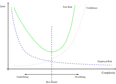
The second term on the right hand side of Eq. 2.9 is an increasing function of h_n and δ. That is, overfitting is very likely to occur as the ratio between the capacity and the number of examples in the training set increases. The capacity plays an interesting role, because a very small capacity can reduce the second term but it might not be good enough to learn the training data, yielding a large empirical risk. On the other hand, a very large capacity will reduce the empirical risk but it will increase the second term. This situation is analogous to the bias-variance dilemma from neural networks and statistics [8]. In order to obtain better generalization, the function space must be restricted such that the capacity is as small as possible, given the available training data. Figure 2.1 shows the intuition behind Eq. 2.9.

Unfortunately, bounds introduced by VC theory are very difficult to measure in prac-tice [8], but they can be exploited using the principle ofstructural risk minimization(SRM). The idea here is to define a nested family of function classes (spaces) _F1 ⊂ · · · ⊂ Fk with

(26)

Empirical Risk True Risk Error Complexity Overfitting Underfitting Confidence Best Model

Fig. 2.1: Illustration of Eq. 2.9. Note how the empirical error decreases with higher capacity but the upper bound on the risk (confidence) becomes worse. The best model lies on the best trade-off between complexity and empirical error.

their corresponding VC dimensions satisfying h1 ≤ · · · ≤ hk. Given this sequence of in-creasingly more complex function spaces, SRM consists of choosing the minimizer of the empirical risk in the function space for which the bound on the structural risk (right hand side of Eq. 2.9) is minimized [25].

2.2 Support Vector Machines

Although bounds as defined previously suffer from practical problems, they offer prin-cipled ways to formulate learning algorithms. SVMs, one of the most well-known classifiers, are built on the basis of SRM. To introduce the basic concepts of SVMs, let us assume that the input space is restricted to X =Rd. Furthermore, under the context of binary classifi-cation, i.e., Y ={−1,+1}, we assume that the data belong to two classes (see Figure 2.2), that can be linearly separableby a hyperplane of the form:

(27)

where the decision surface is parametrized by the weight vector w _∈Rd and the threshold

b∈R, and hw, xi denotes the dot product betweenwand x.

~ w f(x) = 0 f(x) = +1 f(x) =−1 Class+1 Class−1 f(x)<−1 f(x)>+1 x1 x2 1 kwk 1 kwk margin = 2 kwk

Fig. 2.2: A linear classifier separating two classes. The decision surface (in blue) is a hyperplane defined by hw, xi+b= 0. The margin is defined by the distance of the closest points (x1 and x2).

Consider two points x1 and x2 lying on the decision surface, i.e., f(x1) =f(x2) = 0. Then, using Eq 2.10 we obtain _hw,(x1−x2)i = 0, which reveals that the weight vector w is orthogonal to the decision surface; therefore, it determines the orientation of the hyperplane. Additionally, note that the value b

kwk determines the perpendicular distance

from the hyperplane to the origin.

All the hyperplanes satisfying yif(xi) > 0, for all i = 1, . . . , n, can be considered as decision surfaces. With the purpose of selecting the best hyperplane, it turns out that it is possible to restrict the class of hyperplanes using theoretical insights from VC theory. More specifically, the VC dimension can be bounded in terms of the margin. The margin is defined as the minimal distance between an example and the decision surface [8].

A canonical representation of the hyperplane is obtained by rescaling w and b such that the closest points to the decision surface satisfy _|hw, xii+b| = 1. Now consider two points x1 and x2 such that hw, x1i+b = +1 and hw, x2i+b =−1. After projecting both points onto the normal weight vector w

(28)

those projections, i.e., perpendicular to the hyperplane. In consequence, the margin can be expressed in terms of w, because _kw_w_k·(x1−x2) = _k_w2_k. These properties are geometrically illustrated in Figure 2.2 for the cased= 2.

It is proven in [21] that the larger the margin of a function fromF, the smaller its VC dimension. Bear in mind that different functions (hyperplanes) can be defined by simply changingwandb. As the margin of separating hyperplanes expresses the capacity, the SVM algorithm aims at finding the hyperplane parametrization that yields the largest margin for separating all examples in the training set.

2.2.1 Hard Margin

For canonical separating hyperplanes of the form depicted by Eq. 2.10, one can achieve perfect classification of training examples when yi(hw, xii+b) ≥ 1, for i = 1, . . . , n. In other words, when the data are linearly separable, the empirical risk can be kept zero by constraining the parameters w and b. In order to minimize the bound from Eq. 2.9, the complexity term, which increases monotonically with the VC dimension, can be controlled by maximizing the margin. That is, we can minimize the complexity by minimizing _kw_k. This is nicely formulated as the following quadratic optimization problem (also known as theprimal formulation) [8]:

minimize w,b 1 2kwk 2 subject to yi(hw, xii+b)≥1, i= 1, . . . , n. (2.11)

The optimization problem above is convex with linear constraints. We can introduce Lagrange multipliers in such a way that the constraints are replaced by constraints on the multipliers themselves, making the problem easier to handle. Furthermore, in this new formulation, the operations on the examples appear only in the form of dot products. Later, we will generalize the SVM linear model to nonlinear cases by taking advantage of this property.

(29)

each of the constraints defined in Eq. 2.11. To form the Lagrangian, the rule is that for con-straints of the formci ≥0, the constraint equations are multiplied by theα’s and subtracted from the objective function; therefore, from Eq. 2.11 we get the following Lagrangian:

L(w, b, α) = 1 2kwk 2 − n X i=1 αi(yi(hw, xii+b)−1) = 1 2kwk 2₋ n X i=1 αiyi(hw, xii+b) + n X i=1 αi. (2.12)

Once this is a convex quadratic programming problem and those points satisfying the constraints also form a convex set, we can equivalently formulate and solve the dual

problem [28], wherein the solution is determined by minimizing L(w, b, α) with respect to w, b and maximizing it with respect to αi. It follows that, the saddle points are given by the conditions:

∂L(w, b, α)

∂b = 0 and

∂L(w, b, α)

∂w = 0 (2.13)

which after rearrangement of terms translate into: n X i=1 αiyi = 0 and w= n X i=1 αiyixi. (2.14)

A further expansion of terms in Eq. 2.12 yields

L(w, b, α) = 1 2kwk 2₋ n X i=1 αiyihw, xii −b n X i=1 αiyi+ n X i=1 αi (2.15)

where the third term on the right-hand side is zero because of the first condition of Eq. 2.14. In addition, we can get rid ofw by expanding_kw_k2 _{as follows:}

kwk2 ₌_h_{w, w}_i₌ n X i=1 αiyihw, xii= n X i=1 n X j=1 αiαjyiyjhxi, xji. (2.16)

(30)

Accordingly, from Eq. 2.15 and 2.16, the dual problem can be simplified and stated as: maximize α n X i=1 αi− 1 2 n X i,j=1 αiαjyiyjhxi, xji subject to αi≥0, i= 1, . . . , n n X i=1 αiyi = 0 (2.17)

where the solution consists of optimal Lagrange multipliers, denoted byα∗_i. Consequently, the optimum weight vectorw∗ can be recovered by using the vectorα∗ in one of the saddle points shown in Eq. 2.14 as follows:

w∗=

n X

i=1

α∗_iyixi. (2.18)

In the solution, there are particular cases calledsupport vectors. Those are the points lying on one of the hyperplanesf(x) = 1 orf(x) =−1 for whichα∗_i >0, while all training examples that are not support vectors haveα∗

i = 0.

Once we have the optimum weights, the threshold can be determined by considering that for any support vector xi, yi(hw, xii+b) = 1, and thus, b∗ = yi− hw∗, xi. In fact, instead of calculatingb∗for only one support vector, averaging over all support vectors yields a better and more numerically stable solution. With the optimum weights and threshold, the classification rule can be expressed as:

f(x) = sgn (_hw∗, x_i+b∗) = sgn n X i=1 α∗_iyihxi, xi+b∗ ! . (2.19)

In summary, the hard margin formulation of SVMs is applicable when the data are linearly separable. Learning involves solving the optimization problem stated in Eq. 2.17. The solution is known to be sparse, in the sense that, for making new predictions we only have to “remember” the support vectors. Note also that in both the dual formulation (Eq. 2.17) and the classification rule (Eq. 2.19), the data appear in the form of dot products. This is a key observation that later will play a role in the definition of SVMs for nonlinear

(31)

cases.

2.2.2 Soft Margin

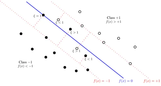
The formulation described in the previous section is applicable when the data are linearly separable, corresponding to an empirical error of zero. Nevertheless, in real world applications, data appear under more complex circumstances and might not be separable by a linear hyperplane. When data from both classes overlap, we need to modify the SVM formulation so as to allow for misclassifications of some training points. The idea is to allow data points to be on the wrong side of the margin; however, they are penalized with an amount proportional to their distance from the margin. To this end, slack variables ξi ≥0 for i= 1, . . . , n, for each training example are introduced [23]. These variables are defined byξi = 0 for points either on the margin or on the correct side of the margin, and ξi =|yi−f(xi)|for all other cases. Points with ξi >1 are misclassified because they lie on the wrong side of the decision surface, and those points for which 0< ξi ≤1 lie inside the margin but on the correct side of the decision surface, as illustrated in Figure 2.3.

f(x) = 0 f(x) = +1 f(x) =−1 Class+1 Class−1 f(x)<−1 f(x)>+1 ξ= 1 ξ <1 ξ <1 ξ >1 ξ >1

Fig. 2.3: Illustration of the slack variables ξi, for i= 1, . . . , n. Note that only the values ξi 6= 0 are shown, corresponding to points on the wrong side of the margin. All the other points lying either on the margin or on the correct side have ξi= 0.

(32)

constraints with the use of slack variables. Hence, the margin has to be maximized in the presence of misclassifications, then the primal problem is formulated in such a way that the VC dimension is small (large margin) while the empirical risk (slack variables) is minimized:

minimize w,b,ξ 1 2kwk 2₊_C n X i=1 ξi subject to yi(hw, xii+b)≥1−ξi, ξi≥0, i= 1, . . . , n (2.20)

where the regularization constant C > 0 is used to determine the tradeoff between the margin and the empirical error. Similar to the case of hard margin SVMs, the primal above can be equivalently written as a dual problem:

maximize α n X i=1 αi− 1 2 n X i,j=1 αiαjyiyjhxi, xji subject to 0≤αi≤C, i= 1, . . . , n n X i=1 αiyi = 0. (2.21)

The dual problem for the soft margin SVM (Eq. 2.21) differs from that of the hard margin (Eq. 2.17) only on the constraints applied to the Lagrange multipliers. In addition, for the soft margin the following observations hold. Data points outside the margin will have α∗_i = 0, while points on the margin line have 0 _≤α∗_i _≤C. Points within the margin have α∗_i = C, including misclassified and correctly classified points. Therefore, support vectors are characterized by 0< α∗_i < C. The optimum values for the weight vectorw∗ and thresholdb∗ can be calculated in the same way as for the hard margin case.

2.3 Kernels

With the introduction of soft margin SVMs, misclassification errors are allowed in order to deal with noisy data. However, in more complex scenarios, the data might not be separable by a hyperplane at all. Thus, the choice of linear functions is, to a certain extent, restricted for learning nonlinearities in the data. We need to generalize the SVM theory

(33)

to deal with nonlinear decision surfaces. Opportunely, the use of kernel functions makes possible training linear models, while at the same time, decision functions are nonlinear. In this section, we provide a short description of kernel functions that serve as important background for the development of later chapters. For the corresponding formal proofs and further details, refer to [29].

2.3.1 Kernel Functions and the Kernel Trick

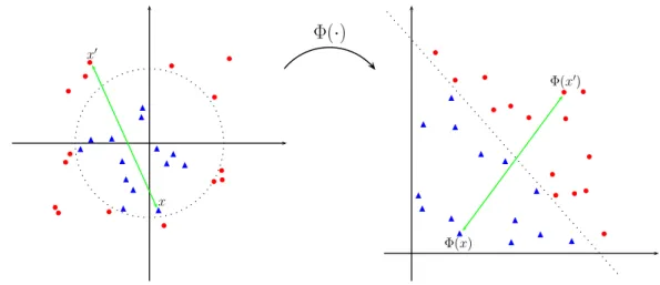
The basic idea is to map theinput space_X into a potentially richer and higher dimen-sionalfeature space_H. The hope is that nonlinear characteristics of the input space become linear in the enlarged space, therefore, allowing for linear separation with hyperplanes. The nonlinear mapping is denoted by a function Φ :X → H called the feature map, illustrated in Figure 2.4. x′ x Φ(x′₎ Φ(x)

Φ(

_·

)

Fig. 2.4: Data points are mapped from an input space X into a feature space H by the function Φ. The dashed boundary shows how data points that are not linearly separable in

X become separable in_H.

We can make any learning algorithm work in the feature space _Hby transforming the input examples into (Φ(x1), y1), . . . ,(Φ(xn), yn)∈ H × Y. Going into a higher dimensional space may appear to suffer from the curse of dimensionality problem, therefore requiring many more examples. However, according to SLT, learning in_Hcan be simpler if one uses a low complexity class of decision functions, for example, classifiers based on hyperplanes [8].

(34)

While it is true that for certain applications we can define and apply an appropriate function Φ(·), the explicit mapping to a higher dimensional space H can be intractable due to the space required and the computational cost involved in the transformation of all examples. It turns out that for certain spaces, there is an attractive way to implicitly calculate dot products in_H without even knowing the function Φ(_·):

k(x, y) =_hΦ(x),Φ(y)_i (2.22)

where k:_{X × X →} R is known as the kernel function. Such a kernel can be intuitively thought of as a similarity measure for any pair of objects from_X.

Learning algorithms can take advantage of kernel functions by implementing thekernel trick. Any algorithm that exclusively uses dot products to interact with input examples from_X can use a kernel function instead to solve the problem in the feature space_H. There is no need to compute the mapping Φ(·) explicitly. For example, the soft SVM from Eq. 2.21 can be extended to a nonlinear space by replacing the dot product hxi, xji with a kernel functionk(xi, xj).

2.3.2 Positive Definite Kernels

In order to make possible similarities in the input space corresponding to dot products in a feature space, kernel functions must bevalid. A valid kernel function satisfiessymmetry, i.e., k(xi, xj) =k(xj, xi), andpositive definiteness in the following sense:

Definition 1 (positive definite kernel) A symmetric function k:X × X →R is a

pos-itive definite 1 kernel if, for any n∈N, x1, . . . , xn∈ X, and c1, . . . , cn∈R

n X

i=1,j=1

cicjk(xi, xj)≥0. (2.23)

1_{In mathematics, functions for which this sum is strictly positive when} _c

i 6= 0 and cj 6= 0 are called

positive definite functions, whereas functions for which this sum is only non-negative are called positive semidefinite functions. For brevity, we will use the term positive definite indifferently for both cases.

(35)

Definition 2 (kernel matrix) Given a positive definite kernel function k and a set of examplesx1, . . . , xn∈ X, then×nmatrixK such thatK(i, j) =k(xi, xj)fori, j= 1, . . . , n

is called the kernel matrix (or gram matrix).

From the definitions above, it follows that if k is a positive definite kernel, we can construct aHilbert space_Hin whichkis a dot product. It is shown in [28] that every kernel function is associated with a Reproducing Kernel Hilbert Space (RKHS) and that every RKHS is associated with a kernel function. Furthermore, Eq. 2.23 is considered essential for practitioners. One of the most powerful kernel methods for classification, the SVM, has the advantage of finding a unique solution. This is only possible when the optimization problem is convex. It turns out that the SVM problem is convex whenever the used kernel matrix satisfies the definitions above.

2.3.3 Properties of Kernels and Examples

Positive definite kernel functions have attractive properties that can be used to create new kernel functions, by combining existing ones. Assuming that _X is an input space and k1 and k2 are arbitrary positive definite kernels defined over X × X, the following are also positive definite kernels: α_·k1, forα >0;k1+k2;k1·k2; and exp(k1).

The distance between two points in the feature space can also be calculated using the kernel trick. Consider two objectsxi, xj ∈ X such that, their respective mappings are Φ(xi) and Φ(xj) in H. The distancedij inHcan be computed as:

dij = kΦ(xi)−Φ(xj)k = (hΦ(xi),Φ(xi)i+hΦ(xj),Φ(xj)i −2hΦ(xi),Φ(xj)i) 1 2 = qk(xi, xi) +k(xj, xj)−2k(xi, xj) (2.24)

wherek is a positive definite kernel function.

It is often a good practice to normalize or scale the training data before applying kernel functions. This is trivial when the data come as a set of vectors, because we can apply the transformation to each column. In a more general case, we only have the kernel

(36)

matrix. Sometimes the kernel matrix is created from objects from a complex input space, not necessarily a Euclidean space. In these cases, it is considered effective to normalize the kernel matrix such that the diagonal elements are all equal to 1, according to:

K(i, j) = p K(i, j)

K(i, i)·K(j, j) for all i, j= 1, . . . , n (2.25) whereK(i, j) denotes the (i, j)th element of the kernel matrixK [30].

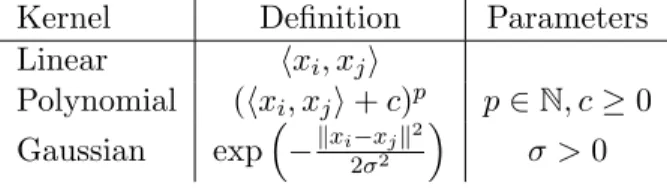
A few instances of kernels for vectorial data have been very popular among SVM practitioners, and they are implemented by default in widely used software packages for SVMs, such as LibSVM2 and SVMlight.3 _{Table 2.1 shows a list of well-known positive} definite kernels.

Table 2.1: List of known positive definite kernels for vectorial data.

Kernel Definition Parameters

Linear _hxi, xji Polynomial (hxi, xji+c)p p∈N, c≥0 Gaussian exp₋kxi−xjk2 2σ2 σ >0

In summary, there are two major benefits in the use of kernels. First, it allows the definition of similarities between arbitrary objects. Once there are no restrictions on the input space X, kernels can be designed for any kind of data, as long as they are valid kernels. For example, several kernels have been proposed to work with complex objects, such as strings, sequences, trees, or graphs (illustrated in Figure 2.5). Second, valid kernel functions can be embedded in any learning task, that is, clustering, classification, regression, or feature extraction, provided that the respective algorithms are based on dot product calculations. For instance, the family of kernel methods includes learning algorithms where observations in the training set only come into the algorithm via dot product calculations with each other.

2

http://www.csie.ntu.edu.tw/~cjlin/libsvm/

(37)

R R R A A A L L T H I

Fig. 2.5: Instances of structured objects, such as sequences, trees and, undirected graphs. One of the major advantages of kernel functions is that they can be defined to measure the similarity between structured objects.

(38)

Chapter 3 Kernels for Graphs

In this chapter, several kernels for graphs are reviewed. Graph kernels are a central topic in this dissertation, since the computational biology problems addressed in later chap-ters are based on graph models of proteins. One can think of graph kernels as similarity functions designed for graph structures. Such similarities must be valid kernels in order to be employed in kernel-based learning tasks as classification or clustering. The design of graph kernels is based on a rich set of fundamentals from graph theory. The challenge is to define similarity measures capable of capturing the structural commonalities between pairs of graphs.

Initially, a brief introduction to graph theory [31] is presented with the purpose of defining terminology and notation for the remaining sections. Next, a brief review of existing algorithms for graph matching is presented (for more details refer to [32]). Then, we present a concise analysis of the major kernel functions for graphs existing in the literature. When possible, we make their connection with graph matching algorithms, as well as highlighting their advantages and shortcomings.

3.1 Introduction to Graph Theory

Formally, agraph Gis defined as a pair _hV, E_i, where V denotes the nonempty set of

vertices (nodes), and E _⊆V _×V denotes the set of edges. An edge e_∈E connects a pair of vertices u, v ∈ V, and it is denoted as (u, v). Theorder of a graph G, denoted by|G|, is defined as the number of vertices in the graph. A graph of order 1 is called trivial. If the vertices or edges of a graph are assigned labels we obtain a labeled graph, sometimes referred to as an attributed graph. When graphs are used to model real world artifacts, e.g., protein structures, the vertices are used to represent entities, and the edges are the

(39)

relationships between pairs of entities.

Vertices u, v ∈ V are adjacent if there exists e = (u, v) ∈ E, where edge e is called

incidentto the vertices uandv. When two vertices are adjacent, they are calledneighbors. The degree of a vertex v is defined as the number of incident edges to v. We define the

adjacency matrixof an unlabeled graphG=_hV, E_iasAn×n= [aij] whereaij = 1 if (vi, vj) is an edge ofGand 0 otherwise.

When the edges in E are ordered pairs of vertices, the graph is called directed. Any directed edge connects asource vertex to a target vertex. Graphs areundirected when the edges in E do not have a particular order or direction. A graph is called simple if there is no edge connecting a vertex to itself (loop) and there are no multiple edges connecting the same pair of vertices. A multigraph is a graph that contains multiple edges. A graph is complete if all of their vertices are connected to each other. The complete graph withn vertices is denoted byKn. Graphs can be represented pictorially, as in Figure 3.1.

A B C D 1 5 2 2 1

Fig. 3.1: Illustration of a graphical representation of graphs. The graph on the left is an undirected graph containing one loop. The graph on the right is a labeled directed and simple graph.

LetG∪G0 =hV ∪V0, E∪E0i and G∩G0 =hV ∩V0, E∩E0i. If G∩G0 =∅, then G and G0 aredisjointgraphs. If V0 ⊆V and E0 ⊆E, thenG0 is a subgraphofG(also written as G0 ⊆G), and G is a supergraph of G0. A complete subgraph from G is referred to as a

clique. If G0 _⊆_G _and _E0 _{contains all the edges} _e_{= (}_{u, v}_{) such that} _e_∈_E _with_{u, v} _∈_V0_,

(40)

Awalkwin a graphGis a nonempty sequence of verticesv1, . . . , vk connected by edges e1, e2, . . . , ek−1such thatei = (vi, vi+1) for all 1≤i < k. Thelengthof a walk is the number of edges in the sequence. If the vertices in the sequence are all distinct, w is called apath

p inG. If v1 =vk in the path p, p is called acycle inG. We can also say that a graph G is connected if for every pair of distinct vertices in G, there exists a path connecting both vertices.

LetG=_hV, E_iandG0 ₌_h_V0_{, E}0_i_{be two graphs. The graphs}_G_and_G0 _are_isomorphic_,

denoted byG_'G0, if there exists a bijectionf:V _→V0with (u, v)_∈E _⇔(f(u), f(v))_∈E0 for all u, v_∈V. The mapf is called an isomorphism. This bijection expresses the general notion of isomorphism being a structure preserving function. However, further restrictions may be imposed so that additional elements are preserved. For example, vertex labels commonly taken from a discrete alphabet. The graph isomorphism relation satisfies the conditions of reflexivity, symmetry, and transitivity [33].

3.2 Graph Matching

Algorithms for graph matching can roughly be classified into two broad categories: methods that aim to determine whether two graphs or subgraphs are identical by means of an exact matching, and methods that are error tolerant by means ofinexact matching[33]. Note that while exact matching for strings, sequences, or vectors are trivial tasks, the same task applied to pairs of graphs is much more complex. Checking if two graphs are identical involves checking if the graphs are isomorphic, or in some cases, if the graphs are identical in terms of topology and labels.

3.2.1 Algorithms Based on Graph Isomorphism

In general, checking isomorphism between graphs demands an exponential computa-tional cost with respect to the number of vertices of the involved graphs. A weaker form of matching is a particular case of isomorphism calledsubgraph isomorphism, which exists between two graphs G and H, if the larger graph H can be turned into a graph that is isomorphic to G by removing some edges and nodes. From this definition it follows that

(41)

Gis contained in H. Note that matching graphs by means of graph and subgraph isomor-phism implies a binary decision, that says whether the graphs are identical or not. This is a shortcoming when the goal is to infer graph similarities. Imagine two graphs that are not isomorphic but present several identical vertices and edges. In such a case, the existing degree of similarity between the graphs is not taken into account by methods based on graph and subgraph isomorphism.

In order to avoid this situation, themaximum common subgraphcan be calculated. Let GandH be graphs, a graphF is called a common subgraph ofGandH ifF is isomorphic to G and H. Then, the maximum common subgraph is the common subgraph with the maximum order. The solution to this problem is not unique, in the sense that there may be several common subgraphs with the same maximum order.

The similarity (or distance) between graphs can be defined in terms of the maximum common subgraph. Intuitively, the larger the common subgraph, the higher the similarity. Although this might work for graphs with discrete labels or unlabeled graphs, the presence of continuous values in labels makes computing similarity between graphs practically im-possible. Imagine two graphs with identical structures consisting of very similar but not identical continuous labels. In this case, the resultant maximum common subgraph is an empty graph, because its calculation relies on isomorphism checks.

All the matching approaches mentioned above are NP-complete, with the exception of graph isomorphism, for which there is no proof that it belongs to the class NP-complete. Al-though polynomial time algorithms exist for particular and constrained instances of graphs, no polynomial time algorithms exist for the general case. Thus, exact matching or at least matching among subparts, has prohibitive time complexity for large graphs in the worst case [32].

3.2.2 Graph Edit Distance

Given the shortcomings of exact graph matching methods, their applicability to real world problems is restricted. To overcome this, several inexact matching methods have been proposed. The idea of inexact matching is that the algorithms evaluate similarities between

(42)

graphs by relaxing the constraints that define the matching. A very common approach along these lines is thegraph edit distance, roughly defined as the cost of the minimum amount of edit operations that is required to transform one graph into the other. A standard set of edit operations include insertions, deletions, and substitutions of both vertices and edges. Graph comparison methods based on edit distance are convenient because they are expressive and they can be applied to arbitrary graphs, where structural errors and continuous labels are allowed. However, they are hard to parametrize and have a high cost associated with time and space complexity. Therefore, these methods are only applicable to relatively small graphs. For a detailed survey of graph edit distance methods, refer to [34].

3.2.3 Graph Embedding

Another approach for graph comparison is graph embedding in vector spaces. The goal is to find feature vector representations in a real vector space Rn for graphs from some graph domain _G. These feature vectors are also referred to as topological descriptors. Formally, embedding is denoted by a function ψ: _{G →} Rn. The motivation for graph embedding methods is that the whole arsenal of pattern recognition tools developed for feature vectors becomes automatically available for the domain of graphs. A popular class of graph embedding methods is based on spectral graph theory [35,36]. Here, graph features are characterized using the spectral decomposition of the Laplacian matrix [36]. A major limitation of methods based on spectral graph theory is that the decomposition is sensitive to structural errors, such as missing or spurious vertices. Furthermore, spectral methods are only applicable to unlabeled graphs or labeled graphs with restricted label alphabets [37].

Recently, a new class of graph embedding methods tolerant to structural errors that allows graphs with arbitrary labels on nodes and edges has been proposed [38]. The basic idea of this approach is the calculation of distances from an input graph G to a number of particular graphs selected from the training set called prototype graphs. The resulting distances are expressed as a vectorial signature ofG. Unfortunately, despite the advantages offered by machine learning tools for vectorial data, methods based on graph embedding still suffer from the high cost in runtime complexity. Computation of topological descriptors may

(43)

require exponential runtime. In fact, graph embedding using prototype graphs resorts to the calculation of graph edit distances between G and the prototypes. Hence, the calculation of optimal solutions is prohibitive for large graphs because the edit distance of graphs is exponential in the number of nodes of the involved graphs. Therefore, the embedding is carried out using approximation algorithms with polynomial time.

3.3 Review of Graph Kernels

Kernel functions for graphs can make the connection between structural data and the powerful set of tools and learning algorithms called kernel methods. Intuitively, a graph kernel is a measure of similarity between two input graphs satisfying the conditions of symmetry and positive definiteness. The formal definition of a graph kernel is given below.

Definition 3 (graph kernel) Let _G be the domain of graphs. The functionk:_{G × G →}R

is called a graph kernel if there exists a Hilbert space H and a mapping Φ : G → H such that:

k(G, G0) =hΦ(G),Φ(G0)i for allG, G0 ∈ G. (3.1)

3.3.1 R-Convolution Kernels

Many of the existing kernels for graphs are based on the seminal idea of R-convolution kernels [39], which provides a general framework for dealing with discrete compound ob-jects. In convolution kernels, complex objects are decomposed into smaller parts, for which a simpler similarity measure can be defined and computed more efficiently. Given the sim-ilarities between the smaller parts, a convolution operation can be used to define a kernel function between a pair of complex objects. Assume that a sample x ∈ X can be decom-posed into parts~x=x1, . . . , xd∈ X1, . . . ,Xd, for example, the decomposition of graphs into subgraphs. We define the relation R, where R(~x, x) is true whenever ~x is a valid decom-position ofx and false otherwise. Now consider the inverse R−1 ₌_{_~x_|_R₍_{~x, x}_{) =}_true_}_{, the}