Transit network design for areas with low and/or heterogeneous demand

(1)

TRANSIT NETWORK DESIGN FOR AREAS WITH LOW

AND/OR HETEROGENEOUS DEMAND

BY

SEYED MOHAMMAD NOURBAKHSH

DISSERTATION

Submitted in partial fulfillment of the requirements

for the degree of Doctor of Philosophy in Civil Engineering

in the Graduate College of the

University of Illinois at Urbana-Champaign, 2014

Urbana, Illinois

Doctoral Committee:

Professor Yanfeng Ouyang, Chair

Professor Rahim F. Benekohal

Professor Bumsoo Lee

(2)

ii

Abstract

Low density and spatial heterogeneity in transit demand impose considerable challenges to both transit riders and service agencies. For example, lower demand forces transit agencies to provide sparser and less accessible service so as to stay economical, which however further deteriorates passenger experience and deters patronage. Spatially heterogeneous demand as well as city street characteristics (e.g., network layout) calls for variation in transit service, which often leads to higher system costs and undesirable passenger experience (e.g., transfers) as well.

This dissertation proposes a series of transit network design methods that can be used to improve transit service under these circumstances. It first presents an alternative flexible-route transit system for low demand areas, in which each bus is allowed to travel across a predetermined area to serve passengers, while these bus service areas collectively form a hybrid “grand” structure that resembles hub-and-spoke and grid networks. We analyze the agency and user cost components of this proposed system in idealized square cities and seek the optimum network layout, service area of each bus, and bus headway to minimize the total system cost. We compare the performance of the proposed transit system with that of other conventional systems (e.g., fixed-route transit network and taxi service), and show which system is advantageous under different passenger demand levels. It is found that under low-to-moderate demand levels, the proposed flexible-route system has the lowest overall system cost.

In the second part of this dissertation, a methodological framework is developed so that continuum approximation (CA) techniques can be used to design bus networks for cities where travel demand varies gradually over space. The bus-route configurations consist of (i) a main,

(3)

iii

city-wide grid with relatively large physical spacings between its parallel routes and the stops along those routes; together with (ii) one or more local grids with more closely-spaced routes and stops that serve neighborhoods of higher-demand densities. The so-called power-of-two concept is borrowed from the field of inventory control, and is enforced so that the local grids can be embedded seamlessly within the main one. Numerical experiments illustrate the value of the resulting heterogeneous route configurations, which have the potential to reduce the costs to both the bus users and the operating agency, as compared against the costs of the optimal homogeneous bus-route grids. Differences of about 5-10% are observed for a set of numerical examples that cover a wide range of demand distribution patterns. Most of the savings are due to the diminished access costs that users incur when high-demand neighborhoods are served by local grids with closely-spaced routes and stops.

The same CA methodology is used to design a simplified grid network system with variable bus spacings that can address spatially heterogeneous demand. The continuum approximation enables us to estimate the cost components of the system locally and design the system layout accordingly. The simplified grid system varies the bus line spacings, which makes the network more responsive to the varying demand. It saves user costs in relatively high demand areas and saves agency costs in lower demand areas. Numerical results show that the design can improve the total cost of the system by between 4% and 6% as compared with traditional grid designs under the chosen demand distribution patterns.

We further extend the network design framework from grid city street networks to a radial one, where buses can travel either radially (from center to outer part and vice versa) or circularly (clockwise and counterclockwise along rings). Using the CA method, we analyze user and

(4)

iv

agency costs and propose a design framework that minimizes the total system cost. The optimum design provides the bus spacings of the radial and circular lines and the bus headway. Numerical results show that the proposed method can be useful to design an efficient system when the city streets form a ring-radial network.

The last part of this dissertation is devoted to real-world applications of the proposed design methods. We apply the flexible-route transit network to satisfying evening/night demand in the campus area of Urbana-Champaign, which is currently covered by a manually dispatched “Safe-Ride” system. The new transit system is shown to outperform the current system and achieve several improvements. We also design a new transit network for the City of Weihai in China, where the network includes both grid and polar network components to best serve the city’s geographical layout. Numerical experiments also give insights on the influence of key decision variables such as bus line spacing, stop spacing, and headway under different design schemes.

(5)

v

Acknowledgments

First, I would like to thank my adviser, Professor Yanfeng Ouyang, for everything he did for me during my Ph.D. study. He patiently, kindly and wisely helped me a lot in every stage of my endeavors. He is my role model not only in academic research but also in life. It was truly a great pleasure for me to study my Ph.D. under his supervision.

I would like to thank Professors Rahim Benekohal, Daniel Work, and Bumsoo Lee for kindly serving as my Ph.D. committee members. I really appreciate their precious time, thoughtful ideas and valuable advice for improving my thesis.

I would like to thank all the Professors with whom I took course during my Ph.D.: Professors Yanfeng Ouyang, Ray Benekohal, Xin Chen, Sheldon Howard Jacobson, Christopher P. L. Barkan, Enlu Zhou, Angelia Nedich, Uday V. Shanbhag, and Ramavarapu Sreenivas. In particular, Professor Yanfeng Ouyang is not only a great adviser but also an excellent teacher. I learned a lot in his classes and I was honored to serve as his TA a few times. I took three courses with Professor Ray Benekohal which expanded my horizon and knowledge in transportation, specially in traffic flow theory and signal systems. I also took three courses with Professor Xin Chen which helped me expand my knowledge in supply chain, inventory and operation research. I would like to thank other colleagues with whom I collaborated in research projects or research papers. In particular I would like to thank Professor Michael J. Cassidy (UC Berkeley) for his great help while co-authoring one of my research papers (also a technical chapter of this dissertation). I also thank Mr. Jay Rank (Champaign-Urbana Mass Transit District) for providing demand data and background information on the campus Safe Ride system. I also would like to thank Leila Hajibabai which I worked with her in “Network Routing for Snow Plows with

(6)

vi

Resource Replenishment” project. During the last two years of my Ph.D., I was honored to work on “Post-Harvest Loss” project in collaboration with department of agricultural and biological engineering. I would like to thank all collaborators in this project: Professor Luis Rodriguez and Yanfeng Ouyang, Dr. Yun Bai, Tao Lin, and Guilherme D. N. Maia.

I would like to thank all former and current students and researchers in our research group to whom I owe a lot to, both in academic and social life: Xiaopeng Li, Fan Peng, Taesung Hwang, Yun Bai, Seungmo Kang, Leila Hajibabai, Xin Wang, Weijun Xie, Eunseok Choi, Jian Wang, Na Cui, Jianxun Cui, Xiaolei Wang, Danfeng Ying, Yajuan Chen, Ping Li, Ryan Smith, Laura Ghosh, YongJe Kim, Daniel Mackowski, Christine Rhodes, Xi Chen, Zhaodong Wang, and Siyang Xie.

Most important, I would like to thank my mother, father, and siblings for their tremendous support and encouragement.

(7)

vii

Chapter 1 Introduction

1.1. Motivation

Transit network design is a critical problem for all the public agencies. The agencies try to provide bus coverage for the entire service region to serve passengers’ needs. The municipality agencies need to plan their public transit system by designing the master plan of the bus route as well as the schedule of the buses. One of the challenges associated with transit network design is the variation of demand over time and space. The demand changes during different hours of a day significantly as well as different days of a week (weekdays and weekends). This variation over time requires designing different transit systems for different periods (e.g., fixed-route and flexible-route for higher and lower demand rate respectively). Usually the transit agency tries to keep their buses running as long as there is enough demand to serve.

Mainly the transit agency designs a fixed-route system based on high demand hours (e.g., from early morning till the evening). During other time, the agency may discontinue some or all of their buses or reduce their frequency. The bus system can be designed as fixed-route for high demand and flexible-route for low demand (when fixed-route is not economic). In this regard, one of the interesting questions is to find the threshold for fixed versus flexible route. Unlike the fixed-route transit network, designing flexible-route transit system that can potentially be used for low demand is one topic that has not been well explored in the literature before.

(10)

2

The first step of transit network design is choosing the proper layout for the transit network. Based on the shape and structure of the service region, different possibilities can be considered as a transit network layout. The grid network is the simplest one in which the buses travel in N-S and E-W directions. Hub-and-spoke is another popular network layout which is common in historical cities. In addition, other transit network layout designs (e.g., radial or multi hub-and-spoke) could be considered. Restricting the design to only one general layout may not be optimum. There are innovative ideas that combine the different layouts to get the advantages of each of them (e.g., combination of grid and hub-and-spoke into a hybrid network; see Daganzo 2010).

In addition to demand variation over time, the demand may also vary over the space. For simplicity, some existing literature assumes uniform demand over the space, but that is not realistic in many cases. To design a transit system while considering heterogeneous demand is another motivation of this dissertation.

Transit network design is in nature a complicated problem and there are many factors that should be taken into account. For example the inconvenience caused by the number of transfers for passengers should be considered in addition of waiting time spent at transfer points. In this dissertation we aim to address all these factors in comprehensive and realistic models, while at the same time, we make reasonable assumptions to maintain simplicity.

(11)

3 1.2. Objectives

The main objective of this Ph.D. dissertation is to design a transit network system that minimizes the total system costs including both transit agency and passenger costs. We investigate the transit network design problem for both flexible-route and fixed-route transit systems. In addition, we consider different service region layouts, shapes, and city streets, as well as heterogeneous demand distribution over space.

To be more specific we first study the flexible-route transit network design that can be economic for lower demand areas. We apply flexible-route where buses pick up and drop off passengers, while we consider a hybrid of grid and hub-and-spoke networks as the overall layout of the system. We analyze all the cost components in order to design the optimum transit system that gives us the transit system specifications including network layout.

We also devote part of this study to analyze the fixed-route transit network. We are looking into the demand variation over the space, and based on that we propose a grid transit network design that is capable of addressing this demand variation either using variable bus spacings or adding local lines. In the variable bus spacings part, we design narrow bus spacings in relatively dense areas and wide spacing in relatively low demand areas in order to reduce the total cost (as compared with uniform spacings) over the entire service region. In local line design, the main concept is to add extra bus lines in higher demand areas and synchronize them with existing bus lines.

In the last technical part of this dissertation we study polar transit systems in mono-centric cities with ring-radial city streets. We attempt to extend our analysis method to design a transit network for circular shape and ring-radial street network cities. We analyze the transit system

(12)

4

cost components, based on which we design the optimum transit network. We also apply the design procedure to hypothetical cases.

For all systems, we apply the proposed models to numerical examples (either real case studies or hypothetical examples) to illustrate how the proposed transit system design works. We further make comparisons among the proposed systems and the transitional ones to show the improvements in user, agency and total system costs.

1.3. Contribution statement

This Ph.D. research studies flexible-route and fixed-route transit network design considering heterogeneous demand distribution over space. Part of this study is devoted to developing a structured flexible-route transit network design for low demand levels and the other part investigates the fixed-route transit system. In the flexible-route transit network design part, we propose the design of flexible-route transit system using the hybrid of grid and hub-and-spoke as the network layout. We obtain closed-form formula for all cost components including transit agency and passengers. Knowing all cost components enables us to design the optimum transit network. We apply the proposed methodology for hypothetical cases and we plan to extend it to real-world cases.

The other part of this study dedicated to designing a transit system with local lines in a grid network context. We propose this idea to address the variable demand by adding extra bus lines to the main grid bus lines where the demand is high. For synchronization and spatial matching of the local and main bus lines, we propose using the power-of-two concept adapted from inventory

(13)

5

control. In addition of the idea of local bus lines, we propose a simplified grid transit network with variable bus spacings. Similarly, we analyze the system cost components and design an efficient transit system based on optimum system cost. We further extend our analysis method and the concept of bus lines with variable spacings to polar transit network. We present methodological framework for designing a polar transit system that buses travel radially (from center to outer part and vice versa) and circularly (clockwise and counterclockwise).

In all the fixed-route cost component analysis, we apply CA method to analyze the system cost components including user and agency costs. This method enables us to analyze the cost components locally and obtain closed-form formula. We further develop heterogeneous designs over space based on minimum cost. Using this powerful tool, we design transit network that can minimizes the total system costs.

In summary, in practical point of view we propose new approaches in transit network design that can be applied to many cities. In academic point of view we propose the application of CA method in transit network design which provides us closed-form formula for all cost components locally and for whole the system. Moreover, we apply the both flexible- and fixed-route to real-world cases.

1.4. Outline

This dissertation is organized as follows. Chapter 2 reviews the related literature and discusses more about the traditional method versus the CA method. Chapter 3 proposes a structured flexible-route transit system for low demand areas. Chapter 4 investigates a transit system design

(14)

6

for demand varying functions over the space including transit system design with local lines. Chapter 5 proposes a simplified grid network system with variable bus spacings. Chapter 6 studies polar transit network design for ring-radial cities. Chapter 7 and 8 design flexible-route transit system for Urbana-Champaign and fixed-route transit system for Weihai, respectively. Finally, Chapter 9 provides concluding discussions and future research directions.

(15)

7

Chapter 2 Literature Review

This chapter first reviews the transit system design literature, including some key methodologies. Then we briefly introduce the CA method which we apply to transit system design models in Chapters 4-6.

2.1. Transit network design

Transit network design is one specific application of transportation network design problem. Network design problems have been extensively studied over the past few decades. Comprehensive reviews can be found in e.g, Friesz (1985) and Yang and Bell (1998). The general transportation network design model can be formulated as follows (Magnanti, 1984):

min ( , )f y (1.a) subject to , , if (k) if (k) , , 0 otherwise k k k i j l i k j N l N R i O f f R i D k K             



(1.b) , , , , , ( , ) A, k i j i j i j i j k K f f K y i j  



   _(1.c) ( , )f y S, (1.d)

(16)

8

 

, 0, , 0,1 , ( , ) A, , i j k i j f  y  i j  kK _(1.e)

where N and A are the sets of nodes and arcs, respectively. Furthermore, set K denotes the commodities and Rk presents the required flow at origin O(k) and destination D(k). We let yi,j be the binary decision variable which is 1 if arc (i,j) is chosen as a part of network design, and 0 otherwise. The continuous decision variable _{i j}_,k

f denotes the flow of commodity k on arc (i,j) and parameter Ki,j shows the capacity of arc (i,j). The objective function (1.a) is general and can be any function. For instance, it can be in the form of a linear function, as follows:

_, _, _, _, ( , ) A ( , ) A ( , ) i jk i jk i j i j k K i j i j f y c f F y     

 





, ₍₂₎

where c_{i j}k_, is the cost of commodity k and Fij is the fixed cost of constructing arc (i,j). The set S in constraint (1.d) can enforce any constraint based on the network design.

On the other hand, transit network design problem has been widely studied in the literature. Several review papers have summarized the transit route network design problem and investigated different aspects of this domain. For example, the most recent literature by Kepaptsoglou and Karlaftis (2009) presented a review research paper on Transit Route Network Design Problem (TRNDP) with the main focus on design objectives, operation environment parameters, and solution approaches. Guihaire and Hao (2008) classified and reviewed the design and scheduling of the network including network design, frequency setting, timetable development, bus and driver scheduling. Desaulniers and Hickman (2007) reviewed public transit design including network design, timetabling, vehicle scheduling, and crew scheduling in operation research point of view. They also summarized a variety of optimization problems that

(17)

9

are related to public transit. Fan and Machemehl (2004) reviewed different transit route network design problems and proposed a model and solution algorithm. Zhao and Gan (2003) presented a review report on the previous studies and developed a model and heuristic solution technique to minimize the number of passengers’ transfers. They also applied their model to some numerical test cases that showed their solution could reduce the average number of transfers. We can also refer to Ceder and Wilson (1986) for a review of different aspects of bus network design models and solution techniques. Chua (1984) reviewed and compared different approaches of urban bus network planning and conducted a survey on the British urban bus operators.

More specifically, the topology of bus networks has been studied as early as the 1960s (e.g., Ceder and Wilson, 1968). The research for a cost-minimizing urban transit system structure (e.g., route positions and headways) explored possible grid networks (Holroyd, 1965), radial systems (Byrne, 1975), and hub-and-spoke systems (Newell, 1979). Wirasinghe et al. (1977) found the optimal network parameters to minimize transit operating cost and passenger travel time in coordinated rail and bus transit systems. Mandl (1980) proposed a method to compute the passenger’s transportation cost and apply it for improving the transit network. Ceder and Israeli (1998) presented a nonlinear mixed-integer program in which the objective function includes both passenger and operator interests. Fan and Machemehl (2006) proposed a multi-objective non-linear mixed integer model and used heuristic methods to solve it. Their objective function is the minimization of both user and agency cost considering unsatisfied demand. To solve that problem they generated an initial route and used genetic algorithm to improve it. The formulation of the transit route construction by Ceder (2007) is presented as follows.

(18)

10 : min _r _r _tr _r r tr r R tr TR c x c  x   



(3.a) , , : 1, , , r tr i j r i j r r tr r R f F a x a  x i j N      



(3.b) , , , ( ) , , r r sp r i j i j i j N c t t r R  



   (3.c) , , , ( ) , , tr tr sp tr i j i j i j N c t t tr TR  



   (3.d) , , 1, , , r tr i j i j r R f F a a i j N      



(3.e) {0,1}, , r x   r R (3.f) , {0,1}, , r i j a   r R (3.g) , {0,1}, , tr i j a   tr TR (3.h)

The objective function introduces the set-covering problem, where it creates a minimum set of routes and their related transfers. Decision variable xr is 1 if route rR is in the solution, and 0 otherwise. a_{i j}r_, (a_{i j}tr_, ) is 1 if the demand (i,j) can be handled directly by route rR (by transfer path trTR) and, 0 otherwise. Constraints (3.c) and (3.d) define cr and ctr as the cost of direct route and transfer path, respectively. Note that t_{i j}r_, , t_{i j}tr_, , and t_{i j}sp_, show the average travel time between i and j on route r, on transfer path tr and on its shortest path, respectively. The sets R, TR, S, Nr, Ntr, Nsp present the transit routes, transfer paths, shortest path, nodes located on route r, nodes located on transfer path tr, and nodes located on shortest path sp, respectively.

(19)

11

The inputs of transit network design model tend to be voluminous, primarily because the inputs entail a good many site-specific details about the system and its operating environment (e.g., Shrivastava and O’Mahony (2006)). Considering many factors as input parameters, solutions (i.e., determinations of the designs that minimize generalized costs) require heuristics and these may come with significant computational costs (e.g., Bagloee and Ceder (2011)).

Furthermore, there are a number of other studies that focused on specific aspects of transit network design, such as mass transit design (Barnett, 2010), bus priority at signalized intersections (Balke et al., 2000), and bus lane priority (Eichler and Daganzo, 2006).

Besides the traditional transit network design, there are some innovative research on system layout or analysis. Models of this type have been used in the design of so-called hybrid transit networks in which routes in the city center are laid-out in a grid structure so that stops enjoy four-directional (N-S and E-W) transit service, while the city’s periphery is covered by a hub-and-spoke structure (Newell, 1979; Wirasinghe, 1977) with two-directional service (Daganzo, 2010a). Compared to the network that features only a grid structure (Holroyd, 1965) or a hub-and-spoke structure (Newell, 1979; Wirasinghe et al., 1977), a hybrid design can often provide service at a lower generalized cost. Subsequent works have shown how an idealized hybrid design can be tailored to suit a real city’s topography (Estrada et al, 2011). Most of these models treat travel demand as a target that is exogenous to the details of the network design. This is not as serious a concern as some readers may think because generalized cost is rather insensitive to demands that vary about the true value (Daganzo, 2010b; 2012).

Moreover, there is some literature that studied the polar transit system design in ring-radial cities. Byrne (1975) developed a transit network model that minimized the user and agency cost.

(20)

12

Morlok and Viton (1984) studied radial urban transit service that can maximize the profit. Vaughan (1986) analyzed the polar network to minimize the total passenger travel time subject to fleet constraints and presented a simple numerical example. There are also some other literature that discuss the transit network design in polar system as a part of their research (e.g., Holroyd (1965) and Black (1978)).

2.2. Continuum Approximation (CA) models

The Continuum Approximation (CA) method for solving transportation problems was first proposed by Newell (1971) for finding optimum headway. He also applied CA method for other transportation fields such as vehicle scheduling or facility location problems (1973). Figure 2.1 shows the cumulative number of arriving and departing passengers for a scheduled transportation system. In this figure, A(t) is the cumulative number of passengers to arrive by time (t), the step function D(t) is the cumulative number of passengers, and D*(t) is the smooth approximation of the D(t) that can be used in CA method. In this context, Daganzo and Newell (1986), using CA method, determined the number of transshipment points and vehicles routing in a network. In the past three decades CA was applied to different aspects of transportation problems. Langevin et al. (1996) and Daganzo (2005) provide an overview of the application of CA method to designing freight distribution systems.

(21)

13

Figure 2.1 Cumulative number vs. time for a transportation system (Newell, 1973).

Daganzo (2005) used the CA method to solve lot sizing problems with variable demand. The CA method can efficiently solve this problem to near-optimal. Figure 2.2.a illustrates the problem which is the cumulative number of items dispatch over time. Curves D(t) and R(t) are the rates of items consumed and received, respectively. Figure 2.2.b illustrates the construction method for cumulative number of items shipped versus time, and by using CA method Figure 2.2.c shows the discretization method for obtaining a set of dispatching times, Hs(t) from continuous dispatching time function, H(t). H(t) can be obtain from the following equation.

1/ 2 2 ( ) ( ) f i c H t c D t     _    , (2)

(22)

14

(a) (b) (c)

Figure 2.2 Lot size problem with variable demand (Daganzo, 2005).

CA algorithm has been used to solve logistics problems including facility location problems as well as network flow problems. Wong (1998) applied CA method for solving network flow of traffic assignment with variable demand. Ouyang and Daganzo (2006) used CA method to solve two dimensional location problem. Later, Li and Ouyang (2010) applied CA method for reliable facility location problem.

In this dissertation, we plan to develop CA modeling framework as a part of solution approaches to transit network design. The general idea of CA method for transit network design is to decompose and calculate the cost components at separate neighborhoods. We assume smooth demand function and based on that we calculate the cost components. Then we can apply optimization techniques to minimize the total system-wide cost over the service region and finally use discretization method to design the transit network.

(23)

15

Chapter 3 A Structured Flexible Transit System for Low Demand Areas

1

3.1. Introduction

Traditionally, transit systems are designed to contain fixed bus routes, and passengers move to predetermined stations to gain access to the system. Very recently, Daganzo (2010) proposed an innovative transit network design framework that determines the adequate structure of the network as well as the optimal headway for a range of transit modes. It was shown that such a hybrid network structure (see Figure 3.1) nicely inherits the advantages of both a hub-and-spoke structure (e.g., low infrastructure investment) and a grid structure (e.g., low travel time).

1_{This Chapter has been adopted from “}_{Nourbakhsh, S.M., Ouyang, Y., 2012. A structured flexible transit system for}

(24)

16

Figure 3.1 A hybrid network structure (Adapted from Daganzo [2010]).

Fixed routes in a transit system provide clarity and regularity to the transit service, and it is known to work very well for densely populated cities (i.e., with high passenger demand) in general. However, in low demand regions (e.g., sprawled suburban areas), the optimal spacing between bus routes often tends to be relatively large so as to reduce the total system cost. As such, the transit system exposes passengers to the open (sometime adverse) environment for a long time while they walk to and from the bus stops. In such cases, adding flexibility to transit route and schedule seems desirable. For example, Quadrifoglio et al. (2006) demonstrated the potential advantages of allowing transit vehicles to travel within a low-demand geographical region to pick up and drop off passengers. Properties of such operations (e.g., bounds on the maximum longitudinal velocity) are obtained, often via simulations, and incorporated into the overall network design via mixed-integer programming models (e.g., Quadrifoglio et al., 2008).

(25)

17

For feeder buses, the suitable demand density for the flexible-route operation is also studied (Quadrifoglio and Li, 2009, among others).

This chapter aims to integrate these interesting ideas (e.g., hybrid network structure, flexible route) into the design of a new structured “flexible-route transit system.” Individual buses operate without fixed routes or predetermined stops, but rather they can travel around within their own service regions to pick up or drop off passengers. At the macroscopic level, however, the buses (or their service regions) collectively form a suitable network structure to provide reliable spatial and temporal service coverage to the entire demand area. In this chapter, instead of relying on complex mathematical programs to determine the optimal network structure numerically, we express the system’s operating performance into analytical functions of a few key design variables, and solve for the optimal design as a simple constrained nonlinear optimization problem. These analytical functions also cast important insights into the impacts of these design variables on the overall system performance. Numerical examples and comparison with comparable alternative systems (e.g., the fixed-route transit system and taxi service) show that the proposed flexible-route transit system is advantageous under a range of low-to-moderate demand levels. This is encouraging because the proposed transit system can be used in a number of real-world applications. One possibility, for example, is to let the transit system switch among different operating modes according to the demand level at specific hours (e.g., at night or during weekend). In addition, the flexible network can be used for design of “safe ride” or “dial-a-ride” systems in which passengers call and wait for pick-ups.

The exposition of this chapter is as follows. Section 3.2 introduces the notation, concept and formulation of the flexible-route transit system. Section 3.3 examines other transit system structures (including the fixed-route transit system and a taxi system) that are comparable to the

(26)

18

proposed one. In Section 3.4, the proposed system is numerically compared with the other systems at different demand levels. Finally, Section 3.5 provides conclusions.

3.2. Methodology

3.2.1. Notation and definition

Similar to Daganzo (2010), we consider a square service region of side D (km) that generates  passenger trips per hour per unit area. The trip origins and destinations are uniform and independently distributed in the region according to a homogeneous spatial Poisson process. The local streets in this service region align along a grid network with constant spacing s.

We consider designing a new flexible transit system to provide service to the passengers when  is relatively small. Unlike the traditional transit system where buses travel along a fixed route and make stops at predetermined stations, in the flexible transit system buses pick up passengers at their origins or drop them off at their destinations. Each bus now serves the passengers in a narrow elongated area, which we call it a “bus tube,” as shown in Figure 3.2(a). The bus makes lateral movements while sweeping longitudinally back and forth through the tube. The exact bus trajectory obviously depends on the realization of passenger locations, but fixed transfer points are planned along each bus tube, and we assume buses always stop at those points.

Figure 3.2(b) shows the grand overview of the structured flexible-route transit system, including the layout of tubes and the location of transfer points. Based on the intended service level, the whole demand area can be divided into the central square and the peripheral quadrants. The transit system includes N-S and E-W hemispheres each containing N equal transit tubes

(27)

19

(with variable width), providing double coverage in the central square and single coverage in the peripheral part2. Obviously, there are N transfer points in each tube (in the inner square) where passengers may transfer to other buses. The central square has a side length of d, and we use the ratio d

D

 to indicate the relative size of the inner square. The maximum width of the tubes (at

the boundary of the entire area) is w D N

 , and the width of the tube inside the central square

equals to w.We further assume that each bus travels in its tube with headway H.

Our design problem is to find the optimal combination of decision variables, [0,1], 0



H , and N{1,2,...}, that minimize the total system costs for the proposed transit system. We further assume that the bus cruising speed is v, the time needed to make one stop (i.e., the delay for acceleration and deceleration) is ₁, the time needed to pick up or drop off a passenger is₂. Since we assume one stop per passenger, the time needed per passenger stop is  , where

1 2

    . As a result, the average bus travel speed (along its flexible trajectory) reduces to v

v_c  . Let C be the capacity of the buses, and  be the factor that captures the discomfort associated with transfers. Passenger can walk at speed v_w.

2

Even though the passenger origins and destinations are assumed to be homogeneous over space and time, it is reasonable to design a higher density of transit network infrastructures near the central part of the city (where most of the traffic is expected to traverse). In the context of many-to-many freight logistics systems, Campbell (1990) showed that the optimal transshipment terminals shall be evenly spaced and yet clustered at the center of the service region.

(28)

20

Figure 3.2. General scheme of the structured flexible transit system.

3.2.2. Formulation

The total system cost mainly consists of two parts: user costs and agency costs. In the following subsections we present formulas for these cost components. Detailed derivations of these formulas can be found in Appendix A.

3.2.2.1 Agency costs

The agency costs include the expected total vehicle distance traveled per hour of operation, Q,

and the expected total fleet size in operation, M. Unlike the fixed-route transit system, the proposed flexible-route system has no specific bus routes or specific locations for picking up or

Transfer point Pick-up or drop-off point Transit trajectory Tube boundary D d w

(29)

21

dropping off passengers, and thus the need for capital infrastructure investments (e.g., building bus stations) is minimal.3 Appendix A shows that the following formula holds for Q:

2 2 3 3 2 2 2 (1 ) 2 2 ( 1) { } (1 ) { } 2 3 p c p i HD l N HD Q D i P i P i D H N N          _        _   _     



 , (1) where { } ! Ds H i N c Ds H P i e i N             , (2) (1 ) (1 ) { } ! Ds H i N p Ds H P i e i N           _ _ , and (3) 3 5 2 2 2 3 3 2 2 5 5 3 3 (1 ) 2 4 , if (1 ) 2 6 (1 ) 3 (1 ) , otherwise (1 )  _{ }         _ _ _ _         _  p D N N D H N N D H D H l N D H . (4)

The bus fleet size, M, is simply given by

/ _c

M Q v , (5)

where the bus average travel speed v_c is given by

2 2 1 1 2 (1 ) 2 c D H N v v QH N     . (6)

Interested readers are referred to Appendix B to see qualitatively how decision variables , N, and H influence agency cost components Q and M.

3.2.2.2. User costs

3_{There may be need for user interfaces (e.g., Internet or phone service systems) and driver communication devices}

(30)

22

The user costs are associated with (i) the total time for passengers to travel from their origins to their destinations, and (ii) other comfort-related factors such as the number of transfers. In the flexible transit system, the total travel time includes the passenger’s waiting time at the origin and possibly at the transfer point(s), and the in-vehicle riding time. Because the passengers are picked up from their exact origins and dropped off at their exact destinations, there is no walking time.

Similar to Daganzo (2010), we assume that the passengers prefer fast and efficient travel. They always choose the travel plan with the least number of transfers, and if transfer is necessary, they transfer at the first opportunity. If there are choices with equal user costs (e.g., regarding the initial direction of travel), they break ties arbitrarily. We further assume that headway control strategies are implemented to stabilize bus schedules such that headway variations at the check points are negligible.4 Under these assumptions, it is shown in Appendix A that the expected waiting time, W, the expected number of transfers, e_T, the expected travel distance, E, the expected in-vehicle travel time, T, for a generic passenger, and the maximum expected vehicle occupancy, O, are given by the following formulas:

4 2 2 1 (1 ) 1 1 2 2 H N W N N          _ _  _  _     , ₍₇₎





2 2 4 1 1 1 2 T N e N N        _  _   , (8)   2 2 2 2 4 ( ) 5 ( ) 2 ( 1) ( ) { } ( ) { } ( ) (1 ) ( ) 3 c p p i HD D E D D i P i P i l N N                          _  _ _   _  



, ₍₉₎

4 Examples of such bus headway control strategies include adaptive holding (Daganzo, 2009) and adaptive cruise speed control (Daganzo and Palioskowski, 2011). Without headway control, the expected passenger waiting time at the transfer points may be larger than half of the headway due to length time bias (Daganzo, 1997).

(31)

23 c E T v  ₍₁₀₎ 2 2 2 4 2 2 1 3 2 3 (1 ) max ; 2 8 32 HD D O N w                 _  _    , (11) where 1 3 5 12 ( ) (11 )        and 1



3



18 ( ) 2 3       .

The maximum expected occupancy is not directly related to user costs. However, it could be useful to the transit agency such that buses with proper capacity (e.g. a van or a mini-bus) can be used.

3.2.2.3. Design

Appendix B shows that the user costs generally decrease with , N and increase with H , but the agency costs generally increase with , N and decrease with H. The optimization problem for the proposed system is to find the best decision variables (central square size), N (the number of tubes in each direction), and H(bus headway) that balance the trade-offs between the agency and user costs;

We convert the agency costs into travel time equivalents. Suppose $_Q is the agency operation cost per vehicle-distance, $_M is the agency cost per vehicle hour, and  is the average monetary value of one passenger-hour, then Q $Q₂

D     and $M₂ M D     convert the

corresponding agency costs into the travel time equivalent per passenger (Daganzo, 2010). We let  measure transfer discomfort, and then

w v



converts the expected transfer number eT into passenger riding time. The optimization problem becomes the following:

(32)

24 Min Q M T w z Q M W T e v         (12) s.t., [1,1] N   , H 0, N{1,2,...



D/s



}.

Note that we enforce   _N1 _and _N 



_D_/_s



_(where_{ }

  is the floor operation) because the central square should contain at least one transfer point, and each tube should contain at least one local street in the longitudinal direction.

To find the optimal value of the objective function, z, we may allow N to take a continuous value and apply numerical nonlinear optimization method (such as the steepest decent method). Numerical approximation is used to estimate the gradient of the objective function.

3.3. Other transportation system structures

In this subsection, we compare the performance of other service providing systems that are comparable to the proposed flexible-route transit system.

3.3.1. Fixed route transit network

In the fixed-route transit system, the total system costs include those related to infrastructure investment, total vehicle distance, bus fleet size, passenger walking time to and from the bus stations, passenger waiting time, and transfer discomfort. To be consistent with our flexible system, and to be conservative (i.e., favoring the fixed-route system), we disregard any possible infrastructure investment in the fixed-route system. The optimization objective can be expressed

(33)

25

in similar notations (while replacing each bus tube by a fixed bus route) as follows (Daganzo, 2010): Min Q M T w z Q M A W T e v          , ₍₁₃₎ where 2 2 2 (3 ) D Q wH     , c Q M v  , 3 2 2 2 (1 ) 3 4 W H     _ _   _  _  ,





3 5 7 12 7 5 3 12 D E       , 3 5 7 1 1 (12 7 5 3 ) 12 c E D T v v w  _ _ _ _     _  _    

  , and the expected walking time is w

w A

v

 . Note that in

the fixed-route system,D

N represents the spacing between adjacent bus routes at the boundary of

the region.

3.3.2. Taxi

For comparison, we consider an idealized situation where “chartered” vehicles (e.g., taxi) deliver each passenger directly from its origin to its destination, and we ignore passenger waiting time at the origin. Hence, the user costs only include the travel time from origin to destination. In the D D square area, the expected travel distance for each passenger is obviouslyE2D/3, and hence the expected travel time per trip is:

v D v E T 3 2   . (14)

Here we have assumed that travel speed v equals the vehicle cruising speed (i.e., ignoring the stopping time to pick up the only passenger). The agency costs depend on the total vehicle-distance per hour of operation, Q, and the fleet size, M. We further ignore any vehicle distance

(34)

26

traveled between delivery trips (e.g., the distance traveled to pick up the next passenger)5, and hence 2 2 3 3 QD E D , and 3 2 3 Q D M v v    . (15)

Then the objective function for the taxi system is:

Min z_QQ_MMT. ₍₁₆₎

It shall be noted that when

2 $_Q Q D     and $M₂ M D   

 , the objective function (16)

becomes 2



$ $



3 Q M

D v

v   , which is independent of the decision variables and demand density. Also note that the minimum user cost, T, by itself provides an absolute lower bound of the system cost for any transportation mode with speed v.

3.3.3. Discussion

Qualitatively, the proposed flexible transit system could be beneficial because it eliminates the need for passengers to walk to the bus stations. This is desirable because it implies a higher level of service to the passengers. In some circumstances (e.g., transit service during night), the benefit also comes from enhanced passenger safety. In addition, the flexible transit system reduces possible need for infrastructure investment, because there are no specific bus lines or stops. However, these advantages may come at a cost: the total vehicle travel distance (and consequently the passenger riding time) could be higher than that in a fixed-route system, because buses also move laterally in their tubes.

5_{This assumption and the other simplified assumptions are in favor of the taxi service and hence conservative for}

(35)

27

As the lateral distance is highly dependent of the number of passengers in the tube, we would expect the flexible-route transit system to be relatively desirable under low demand, while the traditional fixed-route transit system to be desirable under high demand. This intuition is quantitatively verified with the numerical examples in Section 4.

3.4. Numerical analysis

3.4.1. Cost comparison

We compute the optimal system costs of three transit service systems: fixed-route transit, flexible-route transit, and taxi systems, to serve a square area with D=10 km and  varying from 1 to 500 passengers per hour per km2. For comparison, we use parameter values that are either realistically assumed or consistent with those in the literature6, as shown in Table 3.1.

6_{Most parameters in Table 1 are taken from Daganzo (2010), except that we use a smaller value for bus deceleration}

and acceleration time per stop, ₁12 seconds––per Levinson (1983), ₁11.13 seconds on average. We also assume that the spacing between adjacent local streets is s=0.15 km (www.Wikipedia.com).

(36)

28

Table 3.1 Parameters setting for the numerical examples.

Parameter s (km)  ($/hr)  (sec) 1  (sec) 2  (sec) v (km/hr) w v 7 (km/hr)   $Q ($/veh-km) $_M ($/veh-hr) Fixed transit 0.15 20 - 12 1 25 2 0.03 2 40 Flexible transit 0.15 20 13 - - 25 2 0.03 2 40 Taxi - 20 - - - 25 - - 2 40

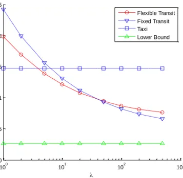
Figure 3.3 plots the optimal cost (per passenger) versus demand density  for the three systems. The cost of the taxi system is independent of . The proposed flexible-route transit system has a lower cost than the fixed-route system when demand is low, while the cost of the fixed-route transit system decreases faster as demand increases. Among the three systems, taxi is desirable under extremely low demand (e.g.,  passengers per hour per km2), while the fixed-route transit system is favorable under high demand. In the middle range when demand is low-to-moderate (e.g., 4~40 passengers per hour per km2), the flexible-route transit system is advantageous. If we realize that the cost functions for the taxi system and for the fixed-route transit system are derived under relatively favorable conditions (e.g., ignoring taxi trips between deliveries and infrastructure investment), then the flexible transit system is probably the best choice for a larger range of demand densities.

7 The average walking distance is normally 3 to 5 km/hr but we consider a lower speed to address the discomfort and delay associated with walking.

(37)

29

Figure 3.3 System cost versus demand density (log-scale).

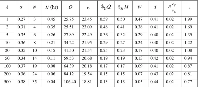
Table 3.2 shows the detail of the optimal design for the proposed flexible-route transit system. When travel demand increases, the optimal size of the central square slightly increase, but the optimal number of tubes increases and the optimal headway decreases considerably as expected. The maximum expected bus occupancy increases at a relatively slow rate, and the average bus velocity decreases only moderately. Almost all agency and user cost components (per passenger) decrease monotonically, except that the number of transfers (and hence the associated cost) remains almost the same.

100 101 102 103 0 0.5 1 1.5 2 2.5  c o s t( h o u r) Flexible Transit Fixed Transit Taxi Lower Bound

(38)

30

Table 3.2 Network design and cost components for the flexible-route transit system.

  N H(hr) O v_c $QQ $MM W T T w e v  _z 1 0.27 3 0.45 25.75 23.45 0.59 0.50 0.47 0.41 0.02 1.99 2 0.31 4 0.35 25.51 23.09 0.48 0.41 0.38 0.41 0.02 1.69 5 0.35 6 0.26 27.89 22.49 0.36 0.32 0.29 0.40 0.02 1.39 10 0.36 8 0.21 34.22 21.95 0.29 0.27 0.24 0.40 0.02 1.22 20 0.35 10 0.15 41.50 21.54 0.25 0.23 0.17 0.40 0.02 1.08 50 0.34 14 0.11 59.53 20.68 0.19 0.19 0.13 0.42 0.02 0.94 100 0.37 19 0.08 64.39 20.18 0.17 0.17 0.09 0.41 0.02 0.87 200 0.36 24 0.06 84.12 19.54 0.15 0.15 0.07 0.43 0.02 0.81 500 0.38 35 0.04 106.40 18.81 0.13 0.13 0.05 0.44 0.02 0.77

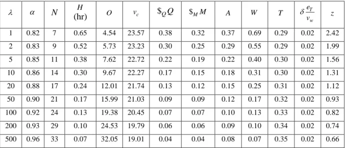
For comparison, Table 3.3 shows the optimal design for the fixed-route system. When travel demand increases, the optimal size of the central square and the optimal number of bus tubes both increase. From Tables 3.2-3.3 we see that the flexible transit system seems to require relatively fewer tubes under lower demand and relatively more tubes under high demand. The maximum expected bus occupancy and average bus speed follow similar trends as those of the flexible transit system. All the agency and user cost components (per passenger) decrease with demand except that the in-vehicle travel time increases slightly (due to a lower bus speed v_c and a higher number of stops N).

(39)

31

Table 3.3 Network design and cost components for fixed-route transit.

  N H (hr) O vc $QQ $MM A W T T w e v  _z 1 0.82 7 0.65 4.54 23.57 0.38 0.32 0.37 0.69 0.29 0.02 2.42 2 0.83 9 0.52 5.73 23.23 0.30 0.25 0.29 0.55 0.29 0.02 1.99 5 0.85 11 0.38 7.62 22.72 0.22 0.19 0.22 0.40 0.30 0.02 1.56 10 0.86 14 0.30 9.67 22.27 0.17 0.15 0.18 0.31 0.30 0.02 1.31 20 0.88 17 0.24 12.01 21.74 0.13 0.12 0.15 0.25 0.31 0.02 1.12 50 0.90 21 0.17 15.99 21.03 0.09 0.09 0.12 0.17 0.32 0.02 0.93 100 0.92 24 0.13 19.38 20.45 0.07 0.07 0.10 0.13 0.33 0.02 0.82 200 0.93 29 0.10 24.53 19.79 0.06 0.06 0.09 0.10 0.34 0.02 0.74 500 0.96 33 0.07 32.05 19.01 0.04 0.04 0.08 0.07 0.35 0.02 0.66

As discussed in Section 3.3, for all, the agency costs in the flexible transit system (Q and M) are larger than their counterparts in the fixed transit system, and each passenger spends more time (T) in the vehicle, because the buses in the flexible system travel extra distances to pick up and drop off passengers. In the flexible transit the ratio of longitudinal over lateral travel over distance varies approximately between 0.54 and 1.67. The advantage of the flexible system is that the passenger walking time (A) is completely eliminated, while the waiting time (W) is also reduced.

For the taxi system, we can easily compute from (16)–(18) that the optimal system cost components are Q=0.67, M=0.53, T=0.27, and hence the system cost per passenger is z=1.47. The agency costs in the flexible transit system (Q and M) are much smaller than that of the taxi system (even under our favorable assumptions), while the taxi system incurs the smallest in-vehicle travel time.

(40)

32

In Section 4.1, we assumed that ₁12 seconds (Levinson, 1983) for both fixed and flexible transit systems. In Daganzo (2010) a more conservative value of ₁ 30 seconds is assumed. Intuitively, longer bus delay per stop will have a direct impact on the total number of buses in operation and the expected travel time per passenger. Such impact will be especially significant for the flexible transit system, because it makes a stop for each passenger visit. To this end, we conduct a sensitivity analysis to see how the three systems perform under ₁ 30 seconds, and the results are shown in Figure 3.4(a). We can see that all curves follow the same trend as those in Figure 3.3, but the optimal costs for the flexible- and the fixed-route transit systems have increased (more so for the flexible system). Although the range of suitable demand for the flexible system has shrunk, we nevertheless notice that the flexible transit system remains the best choice when5~20 passengers per hour per km2.

Under certain circumstances (e.g., adverse weather, night time), passenger walking is associated with significant discomfort or passenger safety becomes a major concern. This situation can be addressed by a dramatic reduction in walking speed v_w. We consider the extreme case when v_wreduces to 0.1 km/hour, and the cost curves are shown in Figure 3.4(b). The total cost for the fixed transit system increases dramatically, mainly due to the increase in walking time (A). The flexible transit system, in contrast, only bears a slight increase in the total cost. The cost for the taxi system remains unchanged. In this case, the flexible transit system becomes favorable for a much larger range of customer demand densities.

Figure 3.4(c) shows the system cost curves under a higher walking speed, 3.0 km/hour. Even with this walking speed the proposed system shows a lower cost for some demand densities. We would like to highlight that the flexible transit system is particularly targeting

(41)

33

situations in which passenger walking is inconvenient (e.g. severe weather condition, night time, or unsafe area). Also note that the actual taxi cost probably much higher than the conservative one shown in this figure; the actual demand range for the flexible system to be optimal is probably much larger.

In the base case the expected waiting time and in-vehicle travel time are assumed to be the same to the passengers. In reality, waiting time is sometimes considered to be less convenient. To study this effect, we consider a case where one unit of waiting time is 1.8 times as costly as in-vehicle travel time. The resulting cost curves are plotted in Figure 3.4(d). Since the relative significance of waiting time in the fixed and flexible route systems are approximately the same, the relative comparison across different systems is similar to that of the base case.

(42)

34

(a)  =30 seconds (b) v_w0.1km/hr

(c) v_w 3.0km/hr (d) (waiting time) = 1.8 (in-vehicle time) Figure 3.4 System cost versus demand density: (a) long bus dwell time; (b) inconvenient walking; (c)

higher walking speed; (d) higher weight of waiting time.

3.5. Conclusion 100 101 102 103 0 0.5 1 1.5 2 2.5  c o s t( h o u r) Flexible Transit Fixed Transit Taxi Lower Bound 100 101 102 103 0 1 2 3 4 5 6 7  c o s t( h o u r) Flexible Transit Fixed Transit Taxi Lower Bound 100 101 102 103 0.2 0.4 0.6 0.8 1 1.2 1.4 1.6 1.8 2 2.2  c o s t( h o u r) Flexible Transit Fixed Transit Taxi Lower Bound 100 101 102 103 0 0.5 1 1.5 2 2.5 3  c o s t( h o u r) Flexible Transit Fixed Transit Taxi Lower Bound

(43)

35

This chapter proposed a structured flexible-route transit system in which buses pick up or drop off passengers within their predetermined service areas (i.e., bus tubes) with no specific routes. Collectively, the bus tubes form a “grand” structure, which includes a grid tube network that provides double coverage to passengers in the central part of the city, and a hub-and-spoke tube network that provides a single coverage in the peripheral part. We analyzed all relevant agency and user costs associated with the system design, and optimized the system by determining the layout of the grand network, the bus tube size, and the bus headway.

The proposed transit system is shown to have the potential to provide a higher level of service to the passengers, mainly by eliminating walking time to and from bus stations. This is particularly desirable under situations where concerns over pedestrian safety are high (e.g., at night or under adverse weather). Quantitative analysis of the proposed system shows that under low-to-moderate passenger demand the system incurs lower cost than other conventional counterparts such as the fixed-route transit system and the chartered taxi system. In practice, the proposed flexible transit system is also easy to implement. The grand structure can be used to guide the tube layout while details of the local streets and neighborhoods are considered. Existing spatial partitioning models (e.g. the disk models in Ouyang and Daganzo, 2006; Ouyang, 2007) can be potentially adapted to help align bus tubes and adjust the size.

Future research could be conducted to explore other network structures (e.g., a ring-radial network) or any hybrid combination of them (e.g. multi-hub-and-spoke). Other shapes of the service region (e.g., rectangle, circle) or heterogeneous demand distributions (e.g., monocentric or multicentric) could be interesting to analyze, although these considerations may add extra complexity to the model.

(44)

36

Chapter 4 Continuum Approximation Approach to Bus Network Design under

Spatially Heterogeneous Demand

8

4.1. Introduction

When designing a public transit system, one would ideally lay-out routes and establish service frequencies in ways that accommodate travel demand at minimum generalized cost to the system’s users and to its operating agency. Most efforts in this realm have relied upon mathematical programming models and numerical solution methods (e.g. Kuah and Perl, 1989; Uchimura, et al, 2002; Lee and Vuchic, 2005; Fan and Machemeh, 2006). These computational burdens often limit the alternatives that are considered in the design process; i.e., the process may consist of only a narrow range of numerical experiments. The resulting insights on how to best design and manage a transit system may equally be narrow.

In efforts to obtain transit designs that are more general and insightful in nature, models have been developed that require fewer and less detailed inputs. Simplicity in this regard is achieved by expressing the inputs and outputs as continuous quantities; e.g. transit routes and the stops along those routes are specified in terms of the physical spacings that separate them, and demand

8_{This chapter has been adopted from “ Ouyang, Y., Nourbakhsh, S.M. and Cassidy, M. (2014)}

“Continuum approximation approach to transit network design under heterogeneous demand.” Transportation Research Part B, 68: 333-344 .”.

(45)

37

for transit travel is expressed as a density, rather than in detailed O-D tables (e.g. Newell, 1973; Daganzo, 1992). In this way, the network design problem for an entire city often conveniently reduces to one that involves only a few key decision variables, such as route and stop spacing and vehicle headway. Solutions to these simpler models can often be obtained analytically, and the resulting insights can be ideal for high-level decision-making. High-level decision-making refers to the strategic and tactical decisions that do not change in the short term (e.g. route and stop spacing and headway).

The simplicity afforded by the above models comes with downsides as well. Of particular concern, these models yield closed-form solutions by treating travel demand as homogeneous over both time and space. This is rarely the case in real settings, however. Fortunately, temporal variations in demand often span periods that are much longer than a vehicle’s headway. Thus, temporal demand variations can often be accommodated relatively easily by operating fleets in flexible manners; e.g. by dispatching buses at frequencies that vary with time of day (Daganzo, 2010b).

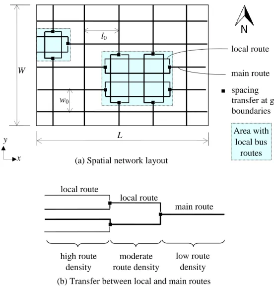
Spatial variations in demand can be more problematic. Variations of this kind often dictate that transit networks display heterogeneous layouts in which some neighborhoods have denser routes and stops than do others. Though Daganzo (2010) offers qualitative design principles for heterogeneous spatial demand, a detailed methodological framework for these cases has not previously been proposed.

The erstwhile absence of a suitable methodology is not surprising. After all, it can be challenging to formulate a design framework that relies on only a few (neighborhood-level) design variables, and that can still produce suitable heterogeneous network configurations. The

Transit network design for areas with low and/or heterogeneous demand