Correlation in Complex Event Processing
Alejandro Grez
Pontificia Universidad Católica de Chile, Santiago, Chile
Millennium Institute for Foundational Research on Data, Santiago, Chile [email protected]
Cristian Riveros
Pontificia Universidad Católica de Chile, Santiago, Chile
Millennium Institute for Foundational Research on Data, Santiago, Chile [email protected]
Abstract
Complex event processing (CEP) has gained a lot of attention for evaluating complex patterns over high-throughput data streams. Recently, new algorithms for the evaluation of CEP patterns have emerged with strong guarantees of efficiency, i.e. constant update-time per tuple and constant-delay enumeration. Unfortunately, these techniques are restricted for patterns with local filters, limiting the possibility of using joins for correlating the data of events that are far apart.
In this paper, we embark on the search for efficient evaluation algorithms of CEP patterns with joins. We start by formalizing the so-called partition-by operator, a standard operator in data stream management systems to correlate contiguous events on streams. Although this operator is a restricted version of a join query, we show that partition-by (without iteration) is equally expressive as hierarchical queries, the biggest class of full conjunctive queries that can be evaluated with constant update-time and constant-delay enumeration over streams. To evaluate queries with partition-by we introduce an automata model, called chain complex event automata (chain-CEA), an extension of complex event automata that can compare data values by using equalities and disequalities. We show that this model admits determinization and is expressive enough to capture queries with partition-by. More importantly, we provide an algorithm with constant update time and constant delay enumeration for evaluating any query definable by chain-CEA, showing that all CEP queries with partition-by can be evaluated with these strong guarantees of efficiency.
2012 ACM Subject Classification Information systems→Data streams; Theory of computation→
Database query processing and optimization (theory); Theory of computation→Formal languages and automata theory; Theory of computation→Automata extensions
Keywords and phrases Complex event processing, Query languages, Correlation, Constant delay enumeration.
Digital Object Identifier 10.4230/LIPIcs.ICDT.2020.14
Funding A. Grez and C. Riveros were partially funded by the Millennium Institute for Foundational Research on Data.
1
Introduction
Streaming query evaluation is the most crucial problem in complex event processing (CEP). Given a CEP queryQ, the streaming evaluation ofQover a stream consists in continuously reading events and outputting all complex events (i.e. sets of events) as soon as the last event that firesQarrives. This streaming evaluation can be divided in two parts: (1) the process that continuously reads events and updates the state of the system whenever a new event arrives and (2) the process that outputs (i.e. enumerates) all complex events that satisfy the query. Both processes are required to run separately in such a way that the update process calls the enumeration process whenever a new output is found [17].
© Alejandro Grez and Cristian Riveros;
licensed under Creative Commons License CC-BY 23rd International Conference on Database Theory (ICDT 2020).
Given the high-throughput data streams in areas like Network Intrusion Detection [27], Industrial Control Systems [19] or Real-Time Analytics [28], the time and space used by these two processes must be severely restricted. As proposed in [7, 17, 22], an efficient streaming evaluation process should satisfy at least the following two ideals: the update process must take constant time per new event and the enumeration process must take constant delay between two consecutive outputs. Intuitively, this is the best that a CEP system can aim for efficiently processing high-throughput data streams in practice. In [17] a streaming evaluation algorithm with constant update time per event and constant delay enumeration was shown for a meaningful core of CEP query languages when only local filters are allowed. Unfortunately, not all relevant queries in CEP can be evaluated with these strong guarantees, which fosters the search of query operators that allow efficient evaluation.
One of the key features in CEP is correlation [12]: to associate different events that might occur arbitrarily far in the input stream. Verifying that two users have the same id, or verifying an increasing sequence of temperature events, are some examples of how correlation is used in CEP. The most basic operator for adding correlation in CEP are equalities, namely, joining two events which have the same data value. Unfortunately, the evaluation of join queries is a difficult task even in a static setting [1], stressing the difficulties of finding efficient evaluation algorithms of CEP queries with equality predicates. One special operator usually included in CEP systems [5, 31, 15] for correlating events is partition-by [5] (also referred assegmentation-oriented context in [16] or justcontext in [15]). As the name suggests, this operator breaks up the events of a stream into partitions where all events of the same partition have the same data value. Despite being a useful operator in CEP, there is a lack of research in evaluating partition-by queries with solid efficiency guarantees, and usually this operator is severely restricted in CEP systems [31].
In this paper, we embark on the search for efficient evaluation of CEP queries with correlation when equality and disequality predicates are used. We first formalize the partition-by operator partition-by extending Complex Event Logic (CEL) [17, 18] with a simple and compositional semantics. To motivate the expressive power of by, we show that CEL with partition-by (but without iteration) is equally expressive as hierarchical queries [7, 22], the biggest subclass of conjunctive queries (CQ) that can be evaluated with constant update time and constant delay enumeration [7].
With a well-defined operator for doing correlation, we study the evaluation of partition-by through a machine model that we called chain Complex Event Automata (chain-CEA), an extension of complex event automata with equality and disequality predicates [17]. Although automata models over data words usually do not have good closure properties [29], we show that the chain-CEA model admits determinization and is expressive enough to capture all CEL queries with partition-by. The most important result of the paper is a streaming evaluation algorithm for the full class of chain-CEA, with constant update time and constant delay enumeration. In particular, this shows that all queries with partition-by can be evaluated efficiently in a streaming fashion.
Related work. Streaming query evaluation has been studied in the context of data stream management systems (DSMS) [5] and complex event processing (CEP) [31, 12, 21]. The notion of constant update time per tuple/event and constant delay enumeration has not been considered until recently [25, 20, 7] and, furthermore, in CEP systems these strong guarantees of efficiency have not been adopted yet [17]. Therefore, the algorithmic approach in CEP systems for evaluating queries with correlation is incomparable to our approach.
New techniques in dynamic query evaluation [8, 2, 9] have recently attracted a lot of attention [7, 22, 23]. In [7, 22], the streaming evaluation of CQ is considered but this does not include queries with order. In [23], inequalities over atoms are considered, but only for
the case of CQ. Our setting also includes disjunction and iteration (but not conjunction), which makes our work orthogonal to the work in [7, 22, 23].
Register automata [24] have been extensively studied in the context of automata theory and XML [29]. Nevertheless, this model has not been studied in the context of CEP and efficient query evaluation. Recently, in [4] a similar extension of complex event automata with registers was proposed. However, this work does not study the determinization and evaluation of this model with constant update time and constant delay enumeration.
2
Preliminaries
In this section, we recall the formal definitions for streams and complex events [17], and give a simplified version of Complex Event Logic (CEL) [18, 17], originally called SO-CEL in [18]. We will later use CEL as a base language to model the partition-by operator.
Streams and complex events. LetAbe a set ofattribute namesandDbe an infinite set of values. A database schemaRis a finite set of relation names, where each relation name
R∈ Ris associated to a tuple of attributes denoted by att(R). IfRis a relation name, then anR-tuple is a function t: att(R)→D. Givena∈att(R), we writet.ato denote the value
t(a), and att(t) to denote dom(t). We say that the type of anR-tupletisR, and denote this by type(t) =R. For any relation nameR, tuples(R) denotes the set of all possibleR-tuples. Similarly, for any database schemaR, tuples(R) =S
R∈Rtuples(R). Given a schema R, an
R-streamS is an infinite sequenceS=t1t2. . . whereti∈tuples(R). WhenRis clear from the context, we refer toS simply as a stream. Given a streamS=t1t2. . . and a position
i∈N, thei-th element of S is denoted byS[i] =ti.
A complex eventCis defined as a non-empty and finite set of natural numbers. Intuitively, given a stream S=t1t2. . .a complex event C={i1, . . . , in} determines the set of tuples {ti1, . . . , tin}and, thus,C represents the set of relevant events. We denote by min(C) and
max(C) the minimum and maximum element ofC, respectively. Given two complex events
C1and C2, we writeC1·C2 for theirconcatenation, which is defined as C1·C2:=C1∪C2 whenever max(C1)<min(C2) and empty otherwise. Given a complex eventC we define
S[C] ={S[i]|i∈C}, namely, the set of tuples inS positioned at the indices specified byC. Complex event logic (CEL). LetXbe a finite set of monadic second-order (SO) variables. An SO predicate of aritynis ann-ary relationP over sets of tuples,P ⊆(2tuples(R))n. We write arity(P) =n. LetPbe a set of SO predicates. An atom overPis an expression of the formP(X1, . . . , Xn) where P ∈Pis a predicate of arity n, and X1, . . . , Xn ∈X(we also writeP( ¯X) forP(X1, . . . , Xn)). A CEL formula is defined by the following syntax:
ϕ := R | ϕINX | ϕFILTERP( ¯X) | ϕORϕ | ϕ;ϕ | ϕ+
whereR ranges over relation names,X over variables inXandP( ¯X) over atoms inP. We sayϕis an atomic formula ifϕ=R.
A valuation is a function µ:X→2Nsuch thatµ(X) is a complex event for everyX ∈X. We define the support ofµby supp(µ) =S
X∈Xµ(X), and the union betweenµ1andµ2 as (µ1∪µ2)(X) =µ1(X)∪µ2(X) for every X ∈X. Given a formula ϕand a stream S, we say that a complex event C belongs to the evaluation of ϕoverS under the valuationµ
(denoted byC∈JϕK(S, µ)) if one of the following conditions holds:
ϕ=R,C={i}, type(S[i]) =R andµ(X) =∅for every X.
ϕ =ρINX, µ(X) =C, and there exists a valuation µ0 such thatC ∈JρK(S, µ
0) and µ(Y) =µ0(Y) for allY 6=X.
type T R R R T R T R . . .
id 123 155 165 223 252 352 355 411 . . .
user-id 11 48 48 48 13 13 33 79 . . .
tweet-id 123 343 123 252 123 . . .
post/reply #vote #ihate #ihate #ihate #vote #ihate #ihate #stop . . .
index 1 2 3 4 5 6 7 8 . . .
Figure 1 A streamS of events from Twitter. T are tweets with an id, a user-id and a post message, andRare responses with an id, a user-id, a tweet-id, and a reply message. The last line is the index of each event in the stream, respectively.
ϕ=ρFILTERP(X1, . . . , Xn),C∈JρK(S, µ) and (S[µ(X1)], . . . , S[µ(Xn)])∈P.
ϕ=ρ1 ORρ2and (C∈Jρ1K(S, µ) orC∈Jρ2K(S, µ) ).
ϕ=ρ1;ρ2 and there exist complex eventsC1 andC2, and valuations µ1 andµ2 such thatC=C1·C2,µ=µ1∪µ2,C1∈Jρ1K(S, µ1) andC2∈Jρ2K(S, µ2).
ϕ=ρ+, andC∈JρK(S, µ) orC∈Jρ;ρ+K(S, µ).
We say that C belongs to the evaluation of a CEL formula ϕ overS at positionn ∈ N,
denoted byC∈JϕKn(S), ifC∈JϕK(S, µ) for some valuationµ, and max(C) =n.
IExample 1. As a running example, suppose that we consider the stream from Twitter. For the sake of simplification, suppose that the stream is composed just by tweets (T) and replies (R). A tweet is composed by three attributes: an id, auser-idand apostmessage. Instead, a reply is composed by four attributes: anid, auser-id, atweet-idof the replied message, and areplymessage. Figure 1 shows an example of a stream with this schema.
As an example of a CEL formula, suppose that a journalist wants to detect all pairs of events composed by a tweet followed by a response containing ‘#voteforjohn’ and ‘#ihatejohn’, respectively, representing “hot” debates in Twitter about the election of a candidate called John. This query can easily be defined with the following CEL-formula:
ϕ1 := (T INX;RINY)FILTER(X.post= ‘#vote’ AND Y.reply= ‘#ihate’)
Here we make use of three operators: sequencing ( ; ) to say we want to find complex events consisting of aT-tuple followed by anR-tuple; variable names (IN) to assign variablesX
andY toT andR, respectively; andFILTERto define the conditions that the events must satisfy. We use conjunction (i.e., AND) as a syntactic sugar, which is short for applying a
FILTERoperator for each predicate of the conjunction. Predicates X.post= ‘#vote’ and
Y.reply = ‘#ihate’ are basically restricting the T and R tuples t and r so that t.post
contains ‘#voteforjohn’ andr.replycontains ‘#ihatejohn’. Given a streamS=t1t2. . .and a valuationµ, one can easily check thatJϕ1K(S, µ) contains complex events of the form{k1, k2} withk1< k2 such thattk1.postcontains ‘#voteforjohn’ andtk2.replycontains ‘#ihatejohn’.
For example,{1,2}, {1,3}and{5,6} in Figure 1 are some outputs ofϕ1 overS. Note that the replies are not necessarily replying to the tweet they are paired with, contrary to what one would like. We address this issue in the next section.
IExample 2. Suppose now that we want to find all sequences of debates that start with a tweet with ‘#voteforjohn’, are followed by one or more responses with ‘#ihatejohn’, and end with a response containing ‘#stophating’. This query can easily be defined in CEL using (+):
ϕ2 = T INX ; R+
INY ; RINZFILTER X.post= ‘#vote’
Inϕ2 we use the (+) operator to extract an unbounded sequence of replies, which are then assigned to Y so that the predicateY.reply = ‘#ihate’ filters only the sequences where all tuples contain ‘#ihatejohn’ (i.e. all tuples t in the complex event represented by Y
must satisfyt.reply= ‘#ihate’). The other predicates are used to ensure that theT-tuple contains ‘#voteforjohn’ and the lastR-tuple contains ‘#stophating’. Finally, one can check thatϕ2defines the desired property. For example, if we evaluateϕ2over Sin Figure 1, then {1,2,4,8} and{1,3,4,6,8} will be some outputs inJϕ2K8(S).
A relevant feature in CEP is to skip arbitrary events when a formula is evaluated [12]. For example, forϕ1it would make no sense looking for two contiguous eventsT andR. For this reason, the sequencing operator allows to skip an arbitrary number of events between two relevant events. The iteration operator has a similar semantics, which results in that for every sequence captured by it, the powerset of events is also captured. To remedy this problem CEL also includes the so-called selection strategies [17, 18], namely, operators for filtering the set of output to a meaningful subset. In this paper, our results do not include the evaluation over selection strategies. We leave this for future work.
CEL fragments and unary predicates. Given a setO of operators (e.g. OR, +), we define CEL[O] to be the set of CEL formulas constructed from atomic formulas,IN, and operators inO. For example,ϕ1 is in CEL[;,FILTER] andϕ2 is in CEL[;,FILTER,+]. Furthermore, we define CEL+Oas the set of all CEL formulas extended withO.
Although CEL does not restrict the set of predicates that can be used byFILTER, not necessarily all predicates can be evaluated efficiently (or are even computable). For this reason, in [18] the analysis of CEL was restricted to SO-extensions of first-order unary predicates. Formally, letU be the set of all unary predicates over tuples, i.e. U={P ⊆tuples(R)}. GivenP ∈Uwe define the SO-extensionPSO⊆2tuples(R)ofP such thatA∈PSO if, and only if,t∈P for allt∈A. We denote byUSOthe set of all SO-extensions of predicates inU. When writing predicates with SO variables we are referring to the SO extension of the first order predicate. For example,P :=x.post= ‘#vote’ is a predicate inUsuch thatt∈P ifft
has the attributepost andt.postcontains #voteforjohn. ThenPSO:= (X.
post= ‘#vote’) is the SO-extension ofP that defines all complex events whose tuples satisfyP.
In [17, 18], it was shown that all CEL formulas restricted to predicates in USO can be evaluated efficiently. For this reason, from now on we assume that for any fragment or extension of CEL, allFILTERare restricted to predicates inUSO.
Streaming evaluation with constant-delay enumeration. As it is standard in the literat-ure [7, 22], we consider evaluation algorithms on Random Access Machines (RAM) with addition and uniform cost measure [3]. Furthermore, we assume the existence of a key-value index (e.g. hash index) that allows insertions and deletions inO(1) time and the index uses space linear in the number of insertions. In other words, we assume to have perfect hashing of linear size [10]. Although this is not realistic for practical computers, it can be simulated with aO(log(n))-factor in the evaluation process with n the number of insertions in the index. Our complexity analysis is always in data complexity, namely, we assume that the CEL query ϕand the schemaRof the stream are fixed. Finally, we restrict the setU to unary predicates with constant time evaluation, namely, for every predicate P inU and every tuplet, we assume that checking whethert∈P takes constant-time.
For efficient evaluation in CEP, we adapt the notion of constant-delay used in [6, 11] for streaming evaluation. Our evaluation process is a streaming algorithm divided in two parts: (1) consuming new events and updating the internal memory of the system and (2)
generating complex events from the internal memory of the system. A streaming evaluation algorithm withconstant update time andconstant-delay enumerationis an algorithm that reads a streamS =t1t2. . .sequentially and evaluates a formulaϕoverS such that (1) the time spent between readingti andti+1 is bounded by O(|ti|), and (2) it maintains a data structureD in memory, such that after readingtn, the setJϕKn(S) can be enumerated from
Dwith constant-delay. The enumeration requires the existence of a routineEnumeratethat enumeratesJϕKn(S) ={C1, C2, . . . , Cm} one by one without repetitions. We call delay(Ci) the time it takes between enumerating Ci and Ci+1, and we sayEnumerate runs with constant-delay if there exists a constantkdepending only onϕsuch that delay(Ci) =k· |Ci| for alli. We remark that (1) is a natural restriction for a streaming algorithm, while (2) is the minimum requirement if an arbitrarily large set of arbitrarily large outputs must be produced [30]. Given that our analysis is in data complexity (i.e. ϕandRare fixed), then the update timeO(|t|) has a hidden factor that depends on|ϕ|and|R|.
3
Partition-by: syntax and semantics
Our main motivation in this paper is to study queries with correlation in CEP. One of the main operators for joining multiple events is partition-by [15, 31] (also referred as segmentation-oriented context in [16] or justcontext in [15]). Intuitively, events in a stream are usually correlated by an attribute that has the same value, e.g. an id. Then this attribute is “partitioning” the stream in multiple streams, where all events of the same stream contain the same value. In this section, we formally define thePART-BYoperator in CEL, and motivate its usefulness by showing that it is expressive enough to define hierarchical queries.
Given two formulas ϕ1 andϕ2, we denote by ϕ1 ⊆ϕ2 when ϕ1 is a subformula of ϕ2. Consider a formulaϕand variablesX1, . . . , Xk ofϕ. We say thatX1, . . . , Xk form avariable cover ofϕif, for every atomic subformulaρof ϕ, i.e. ρ⊆ϕandρ=Rfor someR, there is some i ≤ k and formula ψ = ψ0 IN Xi such that ρ ⊆ ψ ⊆ ϕ, namely, all the events captured by atomic subformulas will be captured by some of the variablesX1, . . . , Xk in ϕ. For example, in Example 2 variablesX,Y andZ form a variable cover ofϕ2.
We extend the syntax of CEL with the operatorPART-BYas follows. A formulaϕis in CEL+PART-BYif it satisfies the syntax of CEL, plus the following rule:
ϕ := ϕPART-BY[X1.a1, . . . , Xk.ak]
whereX1, . . . , Xk ∈X form a variable cover ofϕ anda1, . . . , ak ∈Aare attributes. The semantics of thePART-BYoperator is defined as follows. Consider a complex event C, a streamS =t1t2. . . and a valuationµ. Then, C ∈JϕPART-BY[X1.a1, . . . , Xk.ak]K(S, µ) if
C∈JϕK(S, µ) and for alli, j∈N,l∈µ(Xi) andm∈µ(Xj), it holds that S[l].ai=S[m].aj. Thus, all events must contain the same data value in their attributes. For the case we only want to partition using a single attributeathat is common among all events (e.g. an id), we add the syntactic sugarϕPART-BY[a], which is defined asϕPART-BY[a] := (ϕINX)PART-BY[X.a], whereX is a fresh variable that does not appear inϕ. Clearly,X is a variable cover ofϕ.
IExample 3. In Example 1 we wanted to extract all pairs of tweets and replies that contain #voteforjohn and #ihatejohn, respectively. Althoughϕ1 extract these complex events, it fails to relate a reply with the tweet is replying to. For this, we can use the partition-by operator as follows:
ϕ∗1 := (T INX;RINY)FILTER (X.post= ‘#vote’
Clearly,X, Y form a variable cover ofϕ1. Furthermore,PART-BYrestricts the output to pairs
tandrwitht.id=r.tweet-id. In Figure 1 now only{1,2},{1,4}and{5,6}are inJϕ∗1K(S).
IExample 4. Now, we want to restrict formulaϕ2in Example 2 in order to correlate tweets and replies in a meaningful way. Suppose that we want to restrictϕ2 such that all replies are replying toT and all #ihatejohn replies are from the same user. Then we can extendϕ2 withPART-BYto impose these restrictions (we omit the filters for the sake of readability):
ϕ∗2 = h T INX ; R +PART-BY(user-id)INY ; R INZFILTER (· · ·)i
PART-BY(X.id, Y.tweet-id, Z.tweet-id) This formula shows the advantage of using nesting ofPART-BY. The internalPART-BYover attributeuser-idrestricts all #ihatejohn replies to have the same identifier, namely, they come from the same user. Then the external PART-BY forces all replies to have the same
tweet-idas the first tweet and, therefore, they are replies of the same tweet. In Figure 1, {1,3,4,6,8} is no longer an output but{1,2,4,8}still is.
Partition-by and hierarchical queries. Partition-by models a join operator that usually appears in CEP systems [5, 15, 31]. Although this operator can be considered rather restrictive, interestingly, it is related to the class of hierarchical queries [13, 26], the biggest class of conjunctive queries without projection that can be evaluated in a streaming fashion [7, 22]. To formally define hierarchical queries we first introduce some notation. Given a database schemaR, we assume an arbitrary total order<over the attribute namesA. ForR∈ Rwith att(R) ={a1, . . . , ak} anda1< . . . < ak, we writeR(x1, . . . , xk) for variablesx1, . . . , xk to denote thatxiis assigned to attributeai. We callR(x1, . . . , xk) an atom. A (full) conjunctive queryQis an expressionR1(¯x1)∧. . .∧Rk(¯xk) where eachRi(¯xi) is an atom (i.e. we restrict our discussion to CQ without projection). Given a conjunctive queryQwithk atoms and a streamS=t1t2. . .we say that a complex eventCsatisfiesQif|C| ≤kand{ti|i∈C} |=Q. We defineJQKn(S) as all complex eventsC that satisfyQand max(C) =n.
From now on, we restrict our analysis to hierarchical conjuctive queries. Specifically, for a variable x define the set atom(x) of all atoms in Q where x is mentioned. Then
Q is hierarchical [13, 26] if for every x and y it holds that either atom(x) ⊆ atom(y), atom(x)⊇atom(y), or atom(x)∩atom(y) =∅. For example, the queryR(x)∧S(x, y) is hierarchical andR(x)∧S(x, y)∧T(y) is not.
Unfortunately, CEL+PART-BYis not enough to capture the expressiveness of hierarchical queries. The reason is that partition-by combined with sequencing forces all events with correlated values to be “adjacent”. On the other hand, hierarchical queries do not impose any order over tuples. For this reason, we consider theALL-operator, a standard CEP operator studied in [18]. Formally, given formulasϕ1andϕ2we define the formula ϕ1 ALLϕ2 such that for a stream S and valuation µ it holds that C ∈ Jϕ1 ALL ϕ2K(S, µ) if there exist complex events C1,C2, and valuationsµ1,µ2 such thatC1∈Jρ1K(S, µ1),C2∈Jρ2K(S, µ2),
C=C1∪C2 andµ=µ1∪µ2. In other words,ALLmakes the pair union of complex events coming from evaluatingϕ1 andϕ2, separately. Interestingly, CEL[ALL,PART-BY] captures exactly the expressiveness of hierarchical queries.
IProposition 5. For every hierarchical queryQ, there is a formulaϕinCEL[ALL,PART-BY] such that JQKn(S) =JϕKn(S)for every stream S and positionn, and vice versa.
The previous proposition shows the motivation of partition-by from the perspective of hierarchical CQ. Although CEL+PART-BY is not enough to capture the expressibility of hierarchical CQ, it shows that partition-by is related with a subclass of CQ that can be evaluated efficiently in a streaming fashion.
q1 q2 q3
T1 R2,id=tweet-id
R1,id=tweet-id
Figure 2 An example of chain-CEA with unary predicatesT1 := type(T)∧post = ‘#vote’,
R1:= type(R)∧reply = ‘#ihate’, andR2:= type(R)∧reply = ‘#stop’.
4
Chain complex event automata
Similarly to [17], we base our evaluation approach on an automata model to represent CEL+PART-BY. We present an automata model, called chain Complex Event Automata (chain-CEA), and show that each formula in CEL+PART-BYcan be represented by this model. In order to express thePART-BYoperator, the automata model needs to be able to handle equality predicates. Given attributesa, b∈Adefine the equality and disequality predicates asPa=b ={(t1, t2)| a∈ att(t1)∧b ∈att(t2)∧t1.a =t2.b} andPa6=b = tuples(R)\Pa=b. A conjunctive binary predicate, or binary predicate for short, is a predicate B that is a conjunction of equality and disequality predicates, i.e.,B =Tni=1(Pai∼bi), whereai, bi∈A and∼i∈ {=,6=}. For simplicity, we usually drop the predicate notation and denoteBsimply asVni=1(ai∼bi). For example, (a=b∧c6=d) represents the predicateB =Pa=b∩Pc6=d, and thus (t1, t2)∈B ift1.a=t2.band, if c∈att(t1) andd∈att(t2), then t1.c6=t2.d. To separate equalities and disequalities fromB, we will usually denoteB=B=∧B6= where B= andB6= are binary predicates composed only by equalities and disequalities, respectively. We denote byB the set of all binary predicates.
A chain complex event automaton(chain-CEA) is a tupleA= (Q,∆, I, F) where Qis a finite set of states, the transition relation ∆ is a set of tuples (p, P, B, q), wherep, q∈Q,
P ∈ U and B ∈ B, and I, F ⊆Q are the initial and final set of states, respectively. A configuration ofAis defined by a state and a position in the stream, i.e. a pair (q, i)∈Q×N.
An initial configuration is a pair (q, i) whereq∈I andi= 0. A runρofAover a stream
S=t1t2. . .is a sequence of configurations: (q0, i0) P1/B1 −−→(q1, i1) P2/B2 −−→. . . Pn/Bn −−→(qn, in) such that (q0, i0) is an initial configuration and, for everyj≤n: ij−1< ij, (qj−1, Pj, Bj, qj)∈∆,
tij ∈Pj and (tij−1, tij)∈Bj, where we consider t0 being the empty tuple with no attributes.
Further, the runρabove induces the complex eventCρ={ij |j >0}. We say thatρis an accepting run ifqn∈F. We define the set of complex events ofAoverS ending at position
nasJAKn(S) ={Cρ|ρis an accepting run ofAand max{C}=n}.
It is worth noting that, even though only conjunctions and negations of equality predicates are allowed, in practice every logical combination (i.e. ∧, ∨ and ¬) can be managed by simulating disjunction using multiple transitions. However, we need this restricted definition to later simplify the evaluation algorithm in Section 5.
IExample 6. Recall our complex events in Example 2 of a tweet with #voteforjohn, followed by one or more responses with #ihatejohn, and ending with a response saying #stophating. Suppose now that instead of correlating all responses with the first tweet, we want to extract a chain of responses, namely, for each contiguous responsesr1 and r2 it holds that
r1.id=r2.tweet-id(i.e. r2 is a reply ofr1). In Figure 2 we show a chain-CEA defining this query. If the automaton is in the initial stateq1 and receives a tweettevent containing #voteforjohn, it moves toq2 and storest. Then for each responsercontaining #ihatejohn whosetweet-idis equivalent to the id of the stored event, it forgets that event and storesr. Finally, when it receives anR-event containing #stophating which is responding the stored event, it reaches a final state.
The previous example shows a meaningful CEP query definable by a chain-CEA. This type of queries are very useful in practice (see for example query (7) in [12]). The next result shows that chain-CEA are expressive enough to cover the class of CEL+PART-BYformulas.
IProposition 7. For any formulaϕin CEL+PART-BY, there exists a chain-CEAA such thatJϕKn(S) =JAKn(S)for everyS andn.
On the other hand, one can show that the chain-CEA from Example 6 cannot be defined by any CEL+PART-BYformula. This, together with Proposition 7, shows that that CEL+PART-BY
is strictly included in the queries defined by chain-CEA.
Like in [17] for CEA, here the determinization of chain-CEA is a crucial property for having efficient streaming evaluation and necessary property for removing duplicate runs that produce the same output. We start by defining our notion of deterministic chain-CEA. Similarly to [17], a deterministic chain-CEA must be “deterministic” with respect to the input and output, namely, given a streamS and a complex eventC, there exists at most one run over S that produces C. Formally, we say that a chain-CEA A = (Q,∆, I, F) is I/O deterministic (or just deterministic) if |I| = 1 and, for every pair of transitions (p, P1, B1, q1)= (6 p, P2, B2, q2), it holds that (P1∩B1[t])∩(P2∩B2[t]) =∅ for every tuplet, whereBi[t] is the set of allt0 such that (t, t0)∈Bi. In other words, the conditions (P1, B1) and (P2, B2) must be disjoint. One can easily check that the chain-CEA from Example 6 is deterministic.
I Theorem 8. Chain-CEA admit determinization, namely, for any chain-CEA A there exists a deterministic chain-CEAA0 such that
JAKn(S) =JA
0
Kn(S)for everyS andn. A natural question that arises from the definition of chain-CEA is whether disequalities are strictly necessary in an automata model for CEP. For example, one can easily see that disequalities are not necessary for defining CEL+PART-BYformulas, since the partition-by operator only requires to check that the same value is used through a contiguous subsequence of the output. In the next result, we show that disequalities are indeed necessary if we want to find an automata model that admits determinization. More precisely, let chain-CEA= be the class of chain-CEA where all transitions are restricted to equalities.
IProposition 9. There exists a chain-CEA= A such that there exists no I/O deterministic chain-CEA= equivalent toA.
We are ready to state the main result of the paper.
ITheorem 10. For every chain-CEA, there exists a streaming evaluation algorithm with constant update time and constant delay enumeration.
By combining Proposition 7 and Theorem 10, we get that for any formula in CEL+PART-BY
there exists a streaming evaluation algorithm with constant update time per tuple and constant delay enumeration. It is important to stress that chain-CEA is more general than CEL+PART-BY, in particular, the chain-CEA in Figure 2 cannot be defined by a CEL+PART-BY
formula, but it can still be evaluated efficiently. We leave open whether there exists a set of predicatesP (likePART-BY) such that CEL+P characterizes what is definable by chain-CEA.
5
A streaming evaluation algorithm for chain-CEA
In this section we show how to evaluate a chain-CEA over a stream with constant update time and constant-delay enumeration. We explain first the main data structures used by the algorithm to later show how to evaluate a chain-CEA.
The run DAG. In our algorithms, we compactly represent sets of runs by using a directed acyclic graph (DAG) annotated with configurations. Formaly, letA= (Q,∆, q0, F) be a deterministic chain-CEA. A run DAGGofA(or just run DAG) is a tupleG= (V, E,⊥, κ) consisting of a finite set of verticesV, a set of edges E⊆V ×V, a special vertex⊥ ∈V, and a functionκthat maps everyv∈V to a configurationκ(v)∈Q×NofA. It is required that the graph (V, E) is acyclic,κ(⊥) = (q0,0), and for everyv∈V there is a directed path fromvto⊥. Furthermore, it is also required that for every (u, v)∈E withκ(u) = (q1, i1) andκ(v) = (q2, i2), it holds that i1> i2.
Intuitively, a vertexvlabeled by κ(v) = (q, i) is encoding the last configuration of a run over a streamS. Moreover, by the last two conditions every path starting inv and ending in⊥is representing a run where configurations are listed in decreasing order. We make this intuition more precise as follows. Letπ =vn, . . . , v1,⊥be a path from v =vn to⊥ inGandκ(vj) = (qj, ij) forj ≤n. Thenκ(⊥), κ(v1), . . . , κ(vn) represents a run ofAand CE(π) ={i1, . . . , in} the complex event defined byπ. We denote by CE(v) the set of all complex events defined by paths fromv to⊥in G, and CE(U) =S
v∈UCE(v) forU ⊆V. Note that there could be two paths starting fromv inGthat define the same complex event in CE(v). We say that a run DAGGissafeif CE(v1)∩CE(v2) =∅for everyv1, v2∈V. Indeed, the safety property allows to enumerate all complex events inGwithout repetitions.
ILemma 11. LetG= (V, E,⊥, κ)be a safe run DAG such that there is a procedure that, given any vertexv ∈V, enumerates its neighborhood {u|(v, u)∈E} with constant-delay. Then there exists a procedure that, givenU ⊆V, it enumerates CE(U)with constant delay.
Therefore, by the previous lemma we can use a safe run DAG to encode the outputs of our evaluation algorithm for chain-CEA and enumerate these outputs with constant delay. An index for binary predicates. In our evaluation algorithm we will need a special index over vertices of a run DAG to efficiently evaluate the binary predicates of a chain-CEA. Given a new eventtand a statep, we want to quickly retrieve all configurations (p, i) that have reachedpand such that (ti, t)∈B for somee= (p, P, B, q)∈∆. The run DAG will encode configurations (p, i), but we will need an index to store ti and quickly “check” (ti, t)∈B.
To define this index, we first need to introduce some notation. LetB =Vni=1(ai∼ibi) be a binary predicate with∼i∈ {=,6=}. Without loss of generality, we assume that all conditions
ai ∼i bi inB are different. Let {(ai, bi)}i be a set of fresh attribute names not used in the schemaR. Given a tuplet, we define the left projection and right projection oftwith respect toB as the tuples ~πB(t) and~πB(t), respectively, with attributes in{(ai, bi)}i such that B~π (t).(ai, bi) =t.ai wheneverai∈att(t) and~πB(t).(ai, bi) =t.bi wheneverbi∈att(t). Otherwise, ifai∈/ att(t) or bi∈/att(t), then ~πB(t).(ai, bi) and~πB(t).(ai, bi) are not defined, respectively. The left and right projections extract the relevant information of a tupletto defineB[t]. To see this, we say that t1 andt2 aretotally different, denoted byt16≡t2, if and only ift1.a6=t2.afor every a∈att(t1)∩att(t2), that is, they are different point-wise.
ILemma 12. Let B = B=∧B6= be a binary predicate. Then (t, t0) ∈B if, and only if,
~π
B=(t) =~πB=(t
0)and ~π
B6=(t)6≡~πB6=(t 0).
With the previous notation, we are ready to define our index of a transition, called the equality-disequality index or ED-index for short. LetG= (V, E,⊥, κ) be a run DAG and let e = (p, P, B=∧B6=, q) be a transition. We define the ED-index Indexe as a set of triples (v, t=, t6=) wherev ∈V andt=,t6= are left projections with respect toB= andB6=, respectively. Intuitively, Indexe will keep all configurations that are at state p and are
Algorithm 1Evaluation of a det. chain-CEAA= (Q,∆, q0, F) and a streamS=t1t2. . .. 1: procedure Evaluation(A,S) 2: Init() 3: fori:= 1to ∞do 4: FireTransitions(i) 5: UpdateIndices(i) 6: Enumerate(∪q∈FUqi) 7: procedure Init( ) 8: G←NewMappingGraph(q0) 9: Uq00← {⊥} 10: for alle0= (q0, P,∅, q)∈∆do 11: Index0e0← {(⊥, t∅, t∅)} 12: procedure FireTransitions(i) 13: for alle= (p, P, B=∧B6=, q)∈∆do 14: (t=, t6=)←(~πB=(ti), ~πB6=(ti)) 15: if ti∈P∧Indexei−1[t=, t6=]6=∅ then 16: v←AddNewVertex(G, q, i) 17: Connect(G, v,Indexie−1[t=, t6=]) 18: Ui q ←Uqi∪ {v} 19: procedure UpdateIndices(i) 20: for alle= (p, P, B=∧B6=, q)∈∆do 21: Indexie←Indexie−1 22: (t=, t6=)←( B~π =(ti), ~πB6=(ti)) 23: for allv∈Ui p do 24: Indexie←Indexie∪ {(v, t=, t6=)}
“waiting” to triggere. More specifically, given a streamS =t1t2. . . if (v, t=, t6=)∈Indexe thenκ(v) = (p, i) and t= = ~πB=(ti) and t6= = ~πB6=(ti). Thanks to Lemma 12, whenever
we want to check if (ti, t)∈B=∧B6= for a new tuple t, we only need to obtain the tuple (v, t=, t6=) from Indexeand check whether t==~πB=(t) and t6=6≡~πB6=(t). This motivates the
following main query of an ED-index: given a pair of tuplest0= andt06=:
Indexe[t0=, t06=] ={v∈V | (v, t=, t6=)∈Indexe ∧t==t0= ∧ t6=6≡t06=} (1) That is, Indexe[t0=, t=60 ] returns all verticesv representing configurationsκ(v) = (p, i) such
that there is a tuplet0 witht0
==~πB=(t 0) andt0 6 ==~πB6=(t 0) and (t i, t0)∈B=∧B6=. We will use the ED-index to store configurations and to quickly return them wheneis fired. The streaming evaluation algorithm. In Algorithm 1 we show how to evaluate a determ-inistic chain-CEA over a stream. The main procedure is Evaluation that receives as input a deterministic chain-CEA A = (Q,∆, q0, F) and a stream S = t1t2. . .. This pro-cedure is composed of four subpropro-cedures: Initfor initializing the main data structures, FireTransitions(i) for firing the transitions in ∆ given a new tupleti,UpdateIndices(i) for updating each Indexegiven the previous tupleti, and, finally,Enumeratefor enumerat-ing all complex events endenumerat-ing at positioni. For the sake of presentation, instead of having a yield function that provides each next tuple in the stream, we explicitly index each new phase byi(i.e. associated to tuple ti) and iterate from 1 to “infinity” (the main for-loop at line 3). Then, given the next tupleti, in eachi-phase we fire the transitions and update the indices withti, and enumerate all complex events at position i. In the sequel, we will first explain the data structures used by the algorithm to later describe each subprocedure.
Algorithm 1 maintains three structures that are used by all subprocedures: the run DAG
G= (V, E,⊥, κ), the ED-indices Indexe for eache∈∆, and set of verticesUq ⊆V for each
q ∈Q. As it was explained before, G will encode runs ofA and Indexe will allow us to quickly evaluate the binary predicate ate. Moreover, for eachq∈Qthe setUq will keep the new verticesv (i.e. configurations) atq. These sets will be useful for updating the indices and enumerating all new results. For the sake of presentation, we assume thatG, Indexe, andUq are defined globally and accessible by all subprocedures.
In each i-phase, the algorithm will update G to represent all runs of A overS until positioni. To that end, it will use the following methods on run DAGs. The first method,
κ(⊥) = (q0,0) and empty sets of verticesV and edgesE. The second method,AddNewVertex, receives an event DAG G and a configuration (q, i), and creates a fresh vertex v with
κ(v) = (q, i), and adds it toV. Finally, the method returns the vertexv. The last method,
Connect, receives as input a run DAG G, a vertexv onG, and a nonempty set of vertices
U ⊆ V, and connects v with each vertex in U, namely, (v, u) is added to E for every
u∈U. Although AddNewVertex andConnectcould temporary break the properties ofG
(e.g. acyclicity), we will use it one after the other and it will be clear that the properties of
Gare always preserved.
For the structures IndexeandUq, the reader might have noticed that in Algorithm 1 we use a superscript IndexieandUi
q. Thisiis denoting the “version” of IndexeandUq at phasei. We assume that each newi-version is always initialized as empty (i.e. Ui
q =∅and Index i e=∅). It is important to note that forUqi we use the indexijust to simplify the presentation (i.e. we could have reuse a setUq in each phase). However, for Indexiethe superscript is crucial to denote the version of Indexe when, for example, a vertex v is connected with the set Indexie[t=, t6=] (see line 17). As it will be discussed later (see Section 6), Indexeis a (partially) persistent data structure [14] and the superscript is denoting thei-version of the structure. We are ready to describe each subprocedure in Algorithm 1. The algorithm starts with Initthat is in charge of initializingG, Index0e, andU0
q before phase 1. For this, a new event DAGGis created and the vertex with the initial configuration⊥is assigned toU0
q0 (recall that Uqi =∅ fori≥0 by assumption). Intuitively, this represents that the initial configuration is ready to start. For initializing Indexe, we assume without loss of generality that all outgoing transitions fromq0 use trivial predicates, namely, B =∅ for every e0 = (q0, P, B, q) ∈∆. Then (⊥, t∅, t∅) is the only triple that must contain Index0e0 witht∅ the empty tuple.
For each new phase i, we callFireTransitions(i) that check for each transitione= (p, P, B=∧B6=, q) whether it can be fired or not given the new tupleti (line 13). For this, we extract fromti its right-projectionst= andt6= with respect toB= andB6=, respectively. Then we check if ti satisfies P and whether there exists a previous configuration (p, j) such that (tj, ti) satisfies B=∧B6=. We do this through Indexe, t=, and t6= by checking if Indexie−1[t=, t=6 ]6=∅. If this is the case, all pairs of configurations (p, j) and (q, i) with
(p, j)∈Indexie−1[t=, t6=] satisfy eand we must extend Gwith a new configuration (q, i) that represents all these new runs. For this, we create a new nodev in Gfor configuration (q, i) and connectv with each vertex in Indexie−1[t=, t6=] (lines 16-17). Finally, the new vertexv is added to the setUqi of new vertices in stateqat phasei.
The next step in phaseiis to update Indexie−1 to its new version Index i
e giventi. For this, we use the setUi
p to update each transitione= (p, P, B=∧B6=, q). More specifically, in UpdateIndices(i) we iterate over each transitione= (p, P, B=∧B6=, q) and make Indexie equal to its previous version. Then, we extract fromti its left-projectionst= andt6= with respect toB= andB6=, respectively, and add (v, t=, t6=) to Indexie for eachv ∈Upi. Recall thatUpi contains all the new vertices added duringFireTransitions(i) and, in particular,
κ(v) = (p, i) for eachv∈Ui
p. AfterUpdateIndices(i) is done, the ED-index Index i
econtains all the relevant information for checkingB=∧B6= in the next phases.
Up to this point, it is straightforward to prove the following invariant after each phasei, which leads to the correctness proof of Algorithm 1.
ILemma 13. Consider {Ui
q}q∈Q andGafter the end of the i-phase. Then, for every run (q0,0),(q1, i1). . . ,(qn, in)ofAoverS within =i, there exist v∈Uqin and a path vn, . . . , v0 inGwithvn=vandv0=⊥such thatκ(vj) = (qj, ij)for everyj≤n. Conversely, for every
v∈Ui
q and every pathvn, . . . , v0 inGwithvn=v andv0=⊥, it holds thatκ(v0), . . . , κ(vn) is a run ofA overS. Moreover, ifAis deterministic, thenGis safe.
The final step at phaseiis to enumerate all complex events of accepting runs. For this, we call the subprocedureEnumerateover the set of vertices∪q∈FUqi. By Lemma 13, we know thatGcorrectly encodes all runs ofAuntil thei-th tuple ofSand, moreover,Gis safe (i.e each complex event is represented by exactly one path in G). Therefore, we can easily enumerate all complex eventsJAKi(S) one-by-one and without repetitions, by enumerating all paths inGstarting at vertices in∪q∈FUqi and ending at⊥.
It is only left to show that Algorithm 1 satisfies constant update time and constant-delay enumeration. To do this, we have to dig deeper into the implementation of Indexe, which is the goal of the last section.
6
A persistent index structure for equalities and disequalities
Fix a transitione= (p, P, B=∧B6=, q). Let (v0, t0, r0),(v1, t1, r1), . . .be a sequence of triples such thatvi is a vertex and ti, ri are tuples for alli∈N. Furthermore, define Index0e=∅ and Indexie= Indexie−1∪{(vi, ti, ri)}. Call (vi, ti, ri) an insertion andithe version of Indexe.
To have constant update time and constant-delay enumeration, Indexe must satisfy the following properties, for every pair of tuplest, rand point in timei∈N:
1. every new insertion in Indexe takes constant time, and
2. for allj≤i, Indexje[t, r] can be can be enumerated with constant-delay.
The last condition implies that Indexeis a persistent data structure [14], namely, it preserves the previous version (i.e. Indexje) of itself whenever it is modified.
We claim that, if Indexe satisfies the above three properties, then Algorithm 1 runs with constant update time and constant-delay enumeration. First, given thatAis fixed, then it is clear that every step of Algorithm 1 can be done in constant time, except lines 15, 17, and 24. Checking whether Indexe[t, r]6=∅ (line 15) or doing an insertion in Indexe (line 24) can be done in constant time by properties (2) and (1), respectively. Furthermore, one can execute
Connect(G, v,Indexie[t, r]) (line 17) in constant time if, instead of coding the graph Gwith adjacency lists, we represent the neighborhood of each vertexv by storing t, r,andi inv
and, because of (2), we can later call Indexie[t, r] whenever needed. Finally, from Lemma 11 we know that, if the neighborhood of each vertex from a safe run DAG can be enumerated with constant delay, then CE(U) can also be enumerated with constant delay. Given that Indexie[t, r] allows to enumerate the neighborhood of each vertex, then the enumeration with constant-delay follows.
In the sequel, we show how to implement Indexein order to satisfy properties (1) and (2).
Case without disequalities. If edoes not have disequalities (i.e. B6= is trivial), then for every (v, t, r) ∈ Indexe, we can drop r and keep only (v, t). To satisfy (1) and (2) we use a key-value index DS where keys are tuples t and each value DS[t] is a list of pairs (u0, i0), . . . ,(un, in) where eachuk is a vertex andik is a “timestamp”, namely, the phase whenuk was inserted. Then, for every new insertion (ui, ti) in phasei, we go toDS[ti] and insert (ui, i) at the end of the list. Finally, for every query of the form Indexje[t] we can go intoDS[t], jump into the pair (uk, ik) withik =j and enumerate (uk, ik), . . . ,(u0, i0) with constant-delay. Recall that by our RAM model of computation, we can find the list DS[t] and find the pair (uk, ik) insideDS[t] in constant time (in the latter case, we need another key-value index forDS[t] that, givenj, finds (DS[t])[j] = (uk, j)). Furthermore, by keeping
a b 1 s1 4 2 s2 4 5 s3 3 2 s4 4 2 s5 3 5 s6 3 5 s7 3 [a] [ab] [b] [ba] a b 1 s1 4 2 s2 4 5 s3 3 2 s4 4 2 s5 3 5 s6 3 5 s7 3 2 s8 3 [a] [ab] [b] [ba]
Figure 3A list of tupless1. . . s7 with the additional bookkeeping to support disequalities.
Case with disequalities. Ifeincludes disequalities (i.e. B6= is non-trivial), then we need to extend our listsDS[t] to support insertions (vi, ti, si) and queries Indexie[t, r]. For this, extend
DS[t] as a list of triples (u0, s0, i0), . . . ,(un, sn, in) whereuk andik are as before, andsk is the tuple for supporting disequalities. Similar to the case without disequalities, for every new insertion (vi, ti, si) at phaseiwe go into the list DS[ti] and insert the triple (vi, si, i) at the end of the list. Then for every query Indexie[t, r] we can jump into the listDS[t], jump into the triple (uk, sk, ik) withik =iand enumerate allulwithl≤ksuch thatsl6≡r(i.e.
slandr are totally different). Of course, this last enumeration step cannot be done with constant delay, unless some extra bookkeeping is added to the data structure. The rest of this section is then devoted to do this.
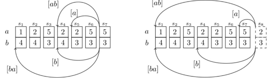
For the sake of simplification, from now on assume that each listDS[t] is composed only by tupless1, . . . , sn. Then the problem is reduced to, given a tuplerand positioni, enumerate the set{sk |k≤i∧sk 6≡r}. Without loss of generality, assume also that alls1, . . . , sn have the same set of attributesA, i.e. att(sk) =A, and define d=|A|. If not, complete each tuplesk with the missing attributes and a fresh value for each new attribute. For example, at the left of Figure 3 we give a lists1, . . . , s7 with attributesA={a, b}andd= 2 where each column is a tuple (over integers) and each row is an attribute.
Let ¯a=a1a2. . . ambe a sequence of non-repeating attributes ofA, and define ¯Ato be the set of all ¯a. For each tuplesk and each ¯a, we define a tuple sk[¯a] =sj withj < k. Strictly speaking,sk[¯a] will be a (backward) pointer fromsk tosj that allows us to jump tosk[¯a] in constant time. Given that our analysis is in data complexity,|A¯|is of constant size, so we only store a constant number of pointers in each tuplesk (although exponential ind). In Figure 3, the pointers [a], [b], [ab], and [ba] ofs7 are displayed with arrows.
Now, for each sk in the list DS[t] =s1, . . . , sn, the tuple sk[¯a] is defined recursively as follows. First, for every attributea ∈ A, sk[a] points to the maximum j < k such that
sk.a6=sj.a. Next, for each sequence ¯a=a1a2. . . am, sk[¯a] points to the maximum j < k such that, for all 1 ≤ l ≤ m, sj.al 6= sk[a1. . . al−1].al where sk[] = sk ( is the empty sequence in ¯A). In the case that there is no such tuplesj, thensk[¯a] is not defined, which means we reached the beginning ofDS[t].
IExample 14. Consider the list s1, . . . , s7 at the left of Figure 3 and consider tuple s7. Thens7[a] =s5 is the last tuple befores7 withavalue different than 5, ands7[ab] =s4 is the last befores7 withs4.a= 26= 5 =s7.aand s4.b= 46= 3 =s5.b. Similarly,s7[b] =s4 is the last node befores7 withs4.b= 46= 3 =s7.b, ands7[ab] =s1is the last befores7 with
With the previous structure overs1, . . . , sn, we show how to enumerate with constant delay the set{sk |k≤i∧sk 6≡r}given a tuplerand indexi. For this, we define a procedure
findNext(sk, r) that returns the last tuplesj withj < ksuch that sj 6≡r (and false ifsj does not exist). Note that, iffindNextruns in constant time, then we can enumerate the set {sk|k≤i∧sk 6≡r}with constant delay: first, ifsi6≡rthen we enumeratesi; then for every last node sk we enumerated, we callfindNext(sk, r) to get the next one, until findNext returns false. For computingfindNext(sk, r), let s:=sk−1be the node immediately before
sk inDS[t]. In the first step we check ifs[] fulfills the condition, namely, if s6≡r. If so, we returns[]; otherwise, there must be some attributea1 such thats[].a1=r.a1. In the next step we consider s[a1] and check ifs[a1].a=6 r.a for eacha∈att(R)\ {a1}; if so, we return s[a1]. Notice we do not need to compare r with all tuples between s[a1] and s[] because, by definition, each tuples0between both satisfys0.a1=s[].a1=r.a1. Furthermore, we no longer need to check the value ofa1 ins[a1] because s[a1].a1 6=s[].a1=r.a1. We repeat this procedure inductively. If we are in step 1 ≤m < d and failed in all previous steps, then for ¯a = a1. . . am ∈ A¯, assume s[a1. . . al−1].al = r.al for every l ≤ m. If
s[¯a]6≡r, returns[¯a]; otherwise consider some attributeam+1∈A\ {a1, . . . , am} such that
s[¯a].am+1=r.am+1. Then we considers[¯a·am+1] in the next step. Again, we do not need to compare r with all elements betweens[¯a·am+1] and s[¯a]: each tuple s0 between both satisfies s0.am+1 =s[¯a].am+1 =r.am+1. Also we do not need to compare s[¯a·am+1] with
r on{a1, . . . , am+1} given that, by induction,s[¯a·am+1].am+1 6=s[¯a].am+1 =r.am+1 and
s[¯a·am+1].al 6=s[a1. . . al−1].al=r.al. At some point we will find some tuple that fulfills the conditions; in the worst-case scenario we iteratedtimes, in which case we are sure by definition thats[a1. . . ad] satisfies the condition or is undefined (i.e. it does not exists). All in all, the procedure takesO(d) steps, which is constant. Moreover, this procedure does not use the pointers ofsk, but the ones ofsk−1. This is an important property that we use next when we want to insert a new node inDS[t].
It is left only to show how to update DS[t] =s1, . . . , sn when we read a new tuple sn+1. For this, we addsn+1 to the end of the list and definesn+1[¯a] for each ¯a∈A¯in the following way. If the list is empty, then sn+1[¯a] is undefined for all ¯a ∈ A¯. Otherwise, for each ¯
a=a1. . . amwe definesn+1[¯a] incrementally over the lengthm. Suppose that,sn+1[a1. . . al] is already defined for every l < m. Define the tupler such thatr.al =sn+1[a1. . . al−1].al for alll < m. Then, definesn+1[a1. . . am] :=findNext(sn+1, r). In other words, we collect all values c1 =sn+1[].a1, c2 =sn+1[a1].a2, . . . , cm =sn+1[a1. . . am].am and find the last tuplessuch thats.al6=cl for everyl≤m. As it was mentioned above, sincefindNextonly uses the pointers ofsn, and not ofsn+1 itself, the function is well-defined. Moreover, given thatfindNext(sn+1, r) can be found in constant time, thensn+1[a1. . . am] is computed in constant time as well.
IExample 15. Suppose that we want to add the node s8={a→2, b→3}to the list on the left of Figure 3. The result is shown on the right of Figure 3 wheres8 is the last dashed column. We defines8[¯a] incrementally usingfindNext. Fora, we callfindNext(n8,{a→2}), which tries with the last tuples7and, because s7.a6= 2, we sets8[a] :=s7. Forb, we call
findNext(s8,{b→ 3}), which first tries withs7, buts7.b= 3, so it tries with s7[b] =s4; sinces4.b6=s7.b, we sets8[b] =s4. For sequenceab, we haves8.a= 2 ands8[a].b= 3, so we callfindNext(s8,{a→2, b→3}). Ass7 conflicts inb, it tries withs7[b] =s4, but this time it conflicts witha, so it tries withs7[ba] =s1. Ass1.a6= 2 ands1.b6= 3, we sets8[ab] =s1. The same procedure is done forba, resulting ins8[ba] =s1.
By combining the key-value indexDSwhere the keys are tuples and the values are the extended list with the additional bookkeeping mentioned above, we get properties (1) and(2) needed for Algorithm 1 to have constant update time and constant-delay enumeration.
7
Future work
This work rises several research opportunities regarding streaming evaluation of queries with correlation in CEP. The first problem is to find a unified class of queries that includes chain-CEA and hierarchical queries. Indeed, there are simple hierarchical queries (e.g.
R(x)∧S(y)∧T(x)) that are not definable by chain-CEA. Another relevant question is whether partition-by queries with projection can be evaluated efficiently. Chain-CEA forbid the use of projection and it is not clear how to extend Algorithm 1 to support it. In particular, it is not clear how to extend this algorithm to support selection strategies [17], an important operator in CEP to filter the number of outputs. Finally, this work studies the streaming evaluation of equality and disequality predicates in CEP, but leaves open the evaluation of other predicates for correlation, like inequalities.
References
1 S. Abiteboul, R. Hull, and V. Vianu.Foundations of databases: the logical level. Addison-Wesley, 1995.
2 Yanif Ahmad, Oliver Kennedy, Christoph Koch, and Milos Nikolic. Dbtoaster: Higher-order delta processing for dynamic, frequently fresh views. Proceedings of the VLDB Endowment, 5(10):968–979, 2012.
3 A. Aho and J. Hopcroft. The design and analysis of computer algorithms. Pearson Education India, 1974.
4 E. Alevizos, A. Artikis, and G. Paliouras. Symbolic Automata with Memory: a Computational Model for CEP. arXiv preprint arXiv:1804.09999, 2018.
5 A. Arasu, S. Babu, and J. Widom. The CQL Continuous Query Language: Semantic Foundations and Query Execution. The VLDB Journal, 2006.
6 Guillaume Bagan. MSO queries on tree decomposable structures are computable with linear delay. InInternational Workshop on Computer Science Logic, pages 167–181. Springer, 2006. 7 C. Berkholz, J. Keppeler, and N. Schweikardt. Answering conjunctive queries under updates.
InPODS, pages 303–318, 2017.
8 Stefano Ceri and Jennifer Widom. Deriving Production Rules for Incremental View Mainten-ance. InVLDB, 1991.
9 Rada Chirkova, Jun Yang, et al. Materialized views. Foundations and Trends® in Databases, 4(4):295–405, 2012.
10 T. Cormen, C. Leiserson, R. Rivest, and C. Stein. Introduction to algorithms. MIT press, 2009.
11 Bruno Courcelle. Linear delay enumeration and monadic second-order logic. Discrete Applied
Mathematics, 157(12):2675–2700, 2009.
12 G. Cugola and A. Margara. Processing flows of information: From data stream to complex event processing. ACM Computing Surveys, 2012.
13 Nilesh N. Dalvi and Dan Suciu. The dichotomy of conjunctive queries on probabilistic structures. InProceedings of the Twenty-Sixth ACM SIGACT-SIGMOD-SIGART Symposium
on Principles of Database Systems, June 11-13, 2007, Beijing, China, pages 293–302, 2007. 14 James R Driscoll, Neil Sarnak, Daniel D Sleator, and Robert E Tarjan. Making data structures
persistent. Journal of computer and system sciences, 38(1):86–124, 1989.
15 Esper Enterprise Edition website. http://www.espertech.com/. Accessed: 2018-12-21. 16 Opher Etzion, Peter Niblett, and David C Luckham. Event processing in action. Manning
Greenwich, 2011.
17 A. Grez, C. Riveros, and M. Ugarte. A formal framework for Complex Event Processing. In
ICDT, 2019.
18 A. Grez, C. Riveros, M. Ugarte, and S. Vansummeren. A Second-Order Approach to Complex Event Recognition. arXiv preprint arXiv:1712.01063, 2017.