Fakultät/ Zentrum/ Projekt XY Institut/ Fachgebiet YZ
12-2018
Institute of Economics
Hohenheim Discussion Papers in Business, Economics and Social Sciences
COMPETITIVENESS AT THE
COUNTRY-SECTOR LEVEL: NEW MEASURES
BASED ON GLOBAL VALUE CHAINS
Martyna Marczak
University of Hohenheim
Thomas Beissinger
Discussion Paper 12-2018
Competitiveness at the Country-Sector Level:
New Measures Based on Global Value Chains
Martyna Marczak, Thomas Beissinger
Download this Discussion Paper from our homepage:
https://wiso.uni-hohenheim.de/papers
ISSN 2364-2084
Die Hohenheim Discussion Papers in Business, Economics and Social Sciences dienen der schnellen Verbreitung von Forschungsarbeiten der Fakultät Wirtschafts- und Sozialwissenschaften.
Die Beiträge liegen in alleiniger Verantwortung der Autoren und stellen nicht notwendigerweise die Meinung der Fakultät Wirtschafts- und Sozialwissenschaften dar.
Hohenheim Discussion Papers in Business, Economics and Social Sciences are intended to make results of the Faculty of Business, Economics and Social Sciences research available to the public in
order to encourage scientific discussion and suggestions for revisions. The authors are solely responsible for the contents which do not necessarily represent the opinion of the Faculty of Business,
Competitiveness at the Country-Sector
Level: New Measures Based on Global
Value Chains
Martyna Marczak
∗University of Hohenheim, Germany
Thomas Beissinger
University of Hohenheim and IZA, Germany
April 26, 2018
Abstract
We propose the so-called domestic “embodied unit labor costs” (EULC) at the country-sector level as a new cost-related basis for measures of international com-petitiveness. EULC take into account that a sector’s labor costs constitute only a small share of its total cost which to a large extent consist of expenses for inter-mediate goods from other sectors. In line with a simple Leontief-type model, the proposed measure is constructed as a weighted average of unit labor costs of all do-mestic sectors contributing to the final goods of a specific sector. The contribution is expressed in value-added terms and takes global supply chains into account. We also show how EULC can be consistently calculated for sectoral aggregates such as the tradable goods sector. Based on EULC we propose the “embodied real effec-tive exchange rate” (EREER) at the country-sector level as a new competieffec-tiveness indicator where the relevance of trading partners is quantified by an appropriate value-added measure. The chosen value-added concept replaces gross exports tra-ditionally used as the weight basis in effective exchange rates. Using the World Input-Output Database (WIOD) we employ the proposed indicators to shed new light on changes in cost competitiveness at the sectoral level for Germany, and compare the empirical evidence with selected other euro area countries.
Keywords: unit labor costs, real effective exchange rate, global supply chains, input-output analysis, sectoral analysis, international competitiveness, WIOD, Germany
JELClassification: J30, C67, E01, F16, F23
∗Corresponding author: University of Hohenheim, Department of Economics, Schloss Hohenheim 1C, D-70593 Stuttgart, Germany. E-mail: [email protected].
1
Introduction
The ongoing debate about causes and consequences of current account imbalances has led to a renewed interest in the competitiveness of nations and industries. A common way to assess external competitiveness is to compare price- or cost-related indicators across countries, typically by means of real effective exchange rates (REERs).1 A cost-related
indicator that is often used for this purpose is unit labor costs (ULC). One advantage of ULC lies in the fact that they reflect changes in competitiveness also in situations where pricing to market prevails, another one is the wide availability of data on wage costs. However, the use of ULC is not free of problems. At the sectoral level, a sector’s own ULC constitute only a small share of total cost which to a large extent consist of expenses for intermediate goods from other sectors. The same problem still emerges at the aggre-gate level if ULC in manufacturing are used as cost indicator for the manufacturing sector or the whole economy. For example, for manufacturing in the euro area the share of ULC in total cost is only about 20 percent (Ca’Zorzi & Schnatz, 2007). Christodoulopoulou and Tkaˇcevs (2014) show that the REER based on ULC in manufacturing behaves differ-ently from other REERs for some euro area countries. This observation strengthens the hypothesis that a too narrow ULC measure may give a misleading picture of changes in international competitiveness.
It has already been noted in the literature that a narrow focus on a sector’s ULC may not reflect its competitive stance. For example, Dustmann et al. (2014) argue that for the period 1995 to 2007 the increase in German competitiveness may be partially explained by the manufacturing sector drawing on inputs from domestically provided nontradable goods and tradable services. Taking account of this argument, we develop a modified ULC measure at the sectoral level that better describes the competitive stance of each sector. The “embodied unit labor costs” (EULC) of a specific sector not only consider that sector’s own ULC but also take account of the ULC incorporated in the intermediate goods delivered to this sector, and therefore are a weighted average of ULC
1Different price- and cost-related REERs are, for example, compared in Marsh and Tokarick (1996),
Chinn (2006), Ca’Zorzi and Schnatz (2007), Christodoulopoulou and Tkaˇcevs (2014) and Fischer et al. (2016). Usually it is found that neither competitiveness indicator clearly outperforms the other.
of all domestic and foreign sectors contributing to the production of this sector. The weights are calculated using global inter-country input-output (ICIO) tables and thus reflect global supply chains. We demonstrate how these weights can be derived from a simple Leontief-type model, and also show how EULC can be consistently calculated for sectoral aggregates, such as the tradable goods sector.
Since statements about the external competitiveness of industries should rely on a comparison of domestic cost (or price) developments with those in other countries, we we consider a re-weighted measure of EULC, called domestic EULC, that is based on contributions of domestic sectors only. However, also in the case of domestic EULC global ICIO tables have to be used because domestic value-added contributions may be embodied in imported intermediate goods.
We then propose a novel measure of REER at the sectoral level that introduces two innovations in comparison to traditional sectoral relative ULC measures: (i) the new measure, called “embodied real effective exchange rate” (EREER), is based on domestic EULC, and thus takes the contribution of other domestic sectors to the competitiveness of a given sector via the intermediate-goods linkages into account, (ii) the weights for com-peting sectors in trading partner countries are based on domestic value added embodied in bilateral sectoral gross exports, which can be seen as a natural value-added counterpart of gross export measures usually used in national-level studies.
Due to the rising importance of global supply chains gross exports no longer constitute the appropriate basis for the weights calculation because they contain foreign value added embodied in intermediates inputs used by the domestic economy to produce gross exports. Moreover, gross exports are “contaminated” by “pure double counting”, i.e. multiple counting of the same value added embodied in intermediates crossing the same border several times.2 For these reasons, an export-related value-added measure is better suited
to calculate weights reflecting the importance of trading partners. A well-known measure is value-added exports which are, for example, used to calculate the VAX ratio (ratio of value-added exports to gross exports) suggested by Johnson and Noguera (2012) as an aggregate measure for the intensity of production sharing. Value-added exports describe
the domestic value added in a country’s gross exports that is ultimately absorbed abroad. However, in our context where the aim is to determine weights for trading partners in the computation of ULC the concept of value-added exports seems not to be a suitable measure. Value-added exports would also partly capture competition with “intermediate” countries along international production chains, whereas our proposed bilateral value-added weights measure competition between direct trade partners and thereby constitute the value-added counterpart of the traditionally used bilateral gross export weights.
For example, value-added exports from the German chemical industry to Italy may reflect intermediate good exports to France that, after reprocessing, are exported to Italy and are absorbed in Italy’s final demand. Hence, the value-added exports of the German chemical industry to Italy consist of a component that is not contained in the gross exports of the German chemical industry to Italy. Our suggested concept reflects solely the value added embodied in the gross exports of the German chemical industry to Italy irrespectively of whether these exports are ultimately absorbed in Italy or any other foreign country.
Koopman et al. (2014) were the first to provide a unified framework for the decom-position of a country’s total gross exports into different value-added and double-counted components. Their framework encompasses various approaches suggested in the litera-ture, such as value-added exports, as special cases. However, their approach only holds at the aggregate level (gross exports of the total economy to all countries) so that it is not readily applicable to the calculation of the domestic value-added content in bilateral gross export flows at the sectoral level.
As Wang et al. (2013) show, a value-added decomposition at the sectoral, bilateral or bilateral sectoral level requires a more demanding framework. The decomposition at the sectoral level is complicated by the fact that domestic value added can be decomposed from the producer’s (forward-linkage) or the user’s (backward-linkage) perspective. The forward-linkage perspective takes into account that a sector’s value added may not only be exported in its own gross exports but also be exported indirectly through gross exports of other domestic sectors. The backward-linkage perspective takes into account that domestic value added embodied in a sector’s gross exports can include value added from
other domestic sectors.
Based on the value-added decomposition suggested in Wang et al. (2013), we calculate the domestic value added in sector-level bilateral gross exports that is absorbed abroad and use that measure in our double weighting scheme to quantify the importance of partner countries at the sectoral level. The value-added concept behind our weight calculation uses the backward-linkage perspective, i.e. it represents the domestic value added in a sector’s gross exports that contains value-added contributions of all domestic sectors. This feature makes it a natural and suitable basis for EREER weights attached to EULC which are also defined in the backward-linkage spirit.
Our suggested EREER measure satisfies the three criteria for any suitable measure of international cost (or price) competitiveness (Durand and Giorno, 1987; Clostermann, 1998): first, the measure should refer to the sectors exposed to international competition -and only those. This is taken into account by deriving the EREER measure at the sectoral level or for suitable sectoral aggregates such as the tradable goods sector. Second, the measure should encompass the overall cost situation of the tradable goods sector. This is accomplished by our concept of EULC. Third, the measure should be constructed from internationally fully comparable data. This is achieved using data from global ICIO tables such as the World Input-Output Database (WIOD) for the derivation of the EREER measure.
Using data from the World Input-Output Database we employ the proposed indicators to shed new light on changes in cost competitiveness at the sectoral level for Germany, and compare the German evidence for the three sectoral aggregates “tradable manufacturing”, “tradable services” and “nontradable goods” with the evidence for other selected euro area countries. Contrary to Dustmann et al. (2014), we show that it is tradable services that profited from more favorable ULC developments in manufacturing and not the other way round. A similar picture emerges if EREERs are compared to standard REERs, where the latter are REERs based on standard ULC and calculated with gross output weights. Regarding the role of the weighting scheme, we show that using value-added weights instead of gross export weights for the sectors in trading partner countries leads to more pronounced increases in international cost competitiveness for both tradable
manufacturing and tradable services in Germany irrespectively of whether EREERs or standard REERs are considered. Hence, the less precise gross exports weights that are used in most of the literature may blur actual chances in cost competitiveness.
The remainder of the paper is organized as follows. Section 2 explains the calculation of EULC and domestic EULC based on global ICIO tables and shows how these measures can be justified in the light of a simple Leontief-type model. It is also shown how domestic EULC can be consistently calculated for sectoral aggregates such as the tradable goods sector. Based on domestic EULC, Section 3 derives EREER as a new REER measure at the sectoral level with value-added bilateral weights for the corresponding sectors in trading partner countries. Section 4 uses data from the World Input-Output Database (WIOD) to calculate EULC and EREER for sectoral aggregates and individual sectors in Germany, and to illustrate the differences compared to standard ULC and standard REER. For the sectoral aggregates the development of EULC and EREER is also com-pared to the corresponding developments in other euro area countries. Section 5 contains a summary and some conclusions.
2
Embodied unit labor costs (EULC)
2.1
EULC based on global ICIO tables
To see how the information contained in global inter-country input-output (ICIO) data-bases can be used to calculate unit labor costs (ULC) embodied in a sector’s production (EULC), the structure of a global ICIO table is explained first. Examples for ICIO databases are the Global Trade Analysis Project (GTAP) and the World Input-Output Database (WIOD).3 Note that an ICIO database can, apart from the ICIO table, contain
supplementary data. LetGdenote the total number of countries andH the total number
3The term “global ICIO” database, also used by Koopman et al. (2014), may be better suited than the
term “global multi-regional input-output (GMRIO)” database often used in the environmental literature, because regional information within countries is not available in those databases. For a description and comparison of global ICIO (GMRIO) databases see, for example, Tukker and Dietzenbacher (2013), Inomata and Owen (2014), and the references therein.
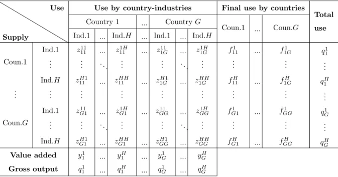
Table 1: The structure of a global ICIO table
Supply
Use Use by country-industries Final use by countries
Total use
Country 1 ... CountryG
Coun.1 ... Coun.G
Ind.1 ... Ind.H ... Ind.1 ... Ind.H
Coun.1 Ind.1 z1111 ... z111H ... z111G ... z1 H 1G f111 ... f11G q11 .. . ... . .. ... ... . .. ... ... ... ... Ind.H zH1 11 ... zHH11 ... z1HG1 ... z HH 1G f H 11 ... f1HG q1H .. . ... ... ... ... ... ... ... ... Coun.G Ind.1 zG111 ... zG1H1 ... zGG11 ... z1GGH fG11 ... fGG1 qG1 .. . ... . .. ... ... . .. ... ... ... ... Ind.H zH1 G1 ... zHHG1 ... zGGH1 ... zGGHH fGH1 ... fGGH qGH Value added y11 ... y1H ... yG1 ... yHG Gross output q1 1 ... q1H ... qG1 ... q H G
of industries. It is assumed that each industry in each country produces one homogenous good that differs from the goods produced by all other industries. For this reason the terms “industry” and “good” can be used interchangeably in the following considerations. With these assumptions in the world a total ofGH goods is produced by the same number of industries.
A global ICIO table basically consists of four parts, see Table 1: (i) the (GH ×GH) matrix Z of intermediate sales (or interindustry sales) describing the intermediate input linkages between all industries of all countries, (ii) the (GH×G) matrixFdenoting final demand, which consists of all GH goods that are sold as final goods to all G countries, (iii) the (GH ×1) vector y of value added of each industry in each country, and (iv) the (GH ×1) vector qof output (or production).
In Table 1 the single elements of these matrices and vectors are denoted in lowercase letters. Throughout the paper, country indices i, j ∈ {1, . . . , G}are written as subscripts and industry indices m, n∈ {1, . . . , H}as superscripts. For example, zmn
ij represents the
intermediate input sales by industry m in country i to industry n in country j. The variablefm
ij denotes final goods produced by sectorm in countryiand sold to countryj.4
As can be seen from Table 1, all gross output produced by sector m in country i must be used as either an intermediate good or a final good either at home or abroad. Therefore, gross output qm
i has to satisfy the following accounting relationship:
qm i = G X j=1 H X n=1 zmn ij + G X j=1 fm ij for i= 1, . . . , G m= 1, . . . , H
This system of equations can also be written in matrix notation:
q=Z·eGH +F·eG, (1)
where eGH and eG denote vectors of ones with dimension (GH ×1) and (G×1),
re-spectively. For the following analysis, the matrix A of technical coefficients (also called input-output coefficients or direct input coefficients) is introduced as
A≡Z·[diag(q)]−1, (2)
where [diag(q)]−1 is a (GH ×GH) diagonal matrix with the elements 1/qn
j on its main
diagonal. The elements of matrixA,amn
ij ≡zmnij /qnj, show how many units of intermediate
inputs industry n in countryj buys from industry m in country i to produce one unit of gross output. In input-output analysis these technical coefficients are taken to be fixed, implying that inputs are used in fixed proportions and economies of scale are ignored.
Since Z=A·diag(q), eq. (1) can be written as
q=A·diag(q)·eGH +F·eG =A·q+F·eG, (3) where q≡ q1 ... qG , A ≡ A11 · · · A1G ... . .. ... AG1 · · · AGG , F≡ F1 ... FG , and qi ≡ q1 i .. . qH i , Aij ≡ a11 ij · · · a1ijH .. . . .. ... aH1 ij · · · aHHij , Fi ≡ f1 i1 · · · fiG1 .. . . .. ... fH i1 · · · fiGH (4)
private consumption or investment. In Table 1 it is assumed that theK final demand components have been summed up tofm.
In input-output analysis the demand (and production) of final goods is considered to be exogenously given. The solution of equation system (3), consisting of GH equations, is
q=B·F·eG, (5)
where the matrix B denotes the so-called Leontief inverse
B≡(IGH −A)−1 = B11 B12 · · · B1G B21 B22 · · · B2G .. . ... . .. ... BG1 BG2 · · · BGG , with Bij ≡ b11 ij · · · b1ijH .. . . .. ... bH1 ij · · · bHHij (6)
IGH denotes the (GH ×GH) identity matrix. The elements bmnij of the Leontief inverse
B are also referred to as “total requirement coefficients” in the input-output literature (Koopman et al., 2014). They show how much output of industry m in country i is needed to produce one extra unit of final good n in country j. Note that this final production satisfies world final consumption (i.e. besides domestic absorption in countryj the exports of the final goodnto other countries are included as well). It must be stressed that in eq. (5) all direct and indirect intermediate good linkages between sectors along international production chains are taken into account.
As a next step, the diagonal matrix V for (direct) sectoral value-added shares is introduced. As is evident from Table 1, total output of a good can also be obtained by summing up value added and all intermediate inputs needed for production. More specifically, it holds that
qn j = G X i=1 H X m=1 zmn ij +y n j forj = 1, . . . , G n= 1, . . . , H In matrix notation q=Z′·e GH +y (7) Since Z′·e
GH = diag(A′ ·eGH)·q, it follows that
y=q−Z′·eGH =V·q, whereV ≡IGH −diag(A′·eGH) = diag(eGH −A′·eGH) (8)
value added in total output of industry n in country j. For later use V is written as V≡ V1 0H,H · · · 0H,H 0H,H V2 · · · 0H,H ... ... . .. ... 0H,H 0H,H · · · VG , with Vj ≡ v1 j 0 · · · 0 0 v2 j · · · 0 ... ... ... ... 0 0 · · · vH j , (9)
where 0H,H is a (H×H) zero matrix, and vjn≡yjn/qjn = [1− PG
i=1
PH
m=1amnij ]/qjn.
The elements of the (GH×GH) matrixV·B represent the value-added contributions of all sectors in all countries to final good production of each sector. For example, the first column ofV·Bcontains the value-added contributions of all sectors in all countries to the final good production of sector 1 in country 1. Note that these value-added contributions take all intermediate input linkages along international production chains into account, i.e. one sector may indirectly contribute to production of another sector by selling inter-mediate goods to third sectors that may also be located in other countries. As will be shown in the next subsection using a simple Leontief type model, the elements of the matrix V·B constitute the weights to calculate the embodied unit labor costs (EULC) of a sector that not only reflect its own ULC, but also ULC of other sectors that are embodied in the intermediate inputs delivered to this sector. The extent to which ULC of other sectors are taken into account depends on the value-added contribution of others sectors to the final good production of this sector. The precise definition is summarized in the following
Definition 1 (Embodied unit labor costs (EULC)). Let u be the (GH ×1) vector containing the unit labor costs of all H sectors in all G countries. Then, an embodied unit labor cost measure for each sector based on its own unit labor costs and the unit labor costs incorporated in the intermediate inputs that a sector receives from all other sectors in all countries is calculated as
uemb
≡Ω′·u, (10)
where Ω≡V·B is the (GH×GH) matrix containing the sector-specific weights for the unit labor costs of all sectors. B is defined in eq. (6) and V in eq. (8).
The relevant weights to calculate EULC for sectornin countryj are in the [(j−1)H+ n]-th column of matrix Ω, with ωmn = vmbmn and PG PH
each element of uemb both the ULC from domestic sectors and those from foreign sectors
are included. However, in the literature the focus often is on the question how domestic wage developments affect the competitiveness of domestic sectors, as has already been outlined in the introduction using Germany as an example. Moreover, as will be shown in Section 3, the calculation of real effective exchange rates is based on a comparison of domestic cost (or price) developments with those of trading partner countries. For these reasons, a modified EULC measure, ue, is proposed that only takes account of the ULC of domestic sectors. Note that domestic ULC may not only be embodied in domestic intermediates but also in imported inputs. For this measure one needs the block diagonal matrix Be that contains the Bii submatrices from matrix B defined in eq. (6), i.e.
e B≡ B11 0H,H · · · 0H,H 0H,H B22 · · · 0H,H .. . ... . .. ... 0H,H 0H,H · · · BGG (11)
Normalizing the weights of the domestic sectoral contributions to production of a specific domestic sector so that their sum equals one gives the following
Definition 2 (EULC based on domestic sectors only (“domestic EULC”)). An EULC measure based on domestic unit labor costs only, i.e. a sector’s own unit labor costs and the unit labor costs embodied in the intermediate inputs that a sector receives from all other domestic sectors, is calculated as
e u =Ωe′·u (12) with e Ω≡(V·Be)·diag([e′GH ·(V·Be)] −1), (13)
where eGH denotes a (GH ×1) vector of ones, V is defined in eq. (8), and Be is defined
in eq. (11).
The matrix Ωe is a block-diagonal matrix
e Ω≡ e Ω11 0H,H · · · 0H,H 0H,H Ωe22 · · · 0H,H .. . ... . .. ... 0H,H 0H,H · · · ΩeGG (14)
where a single element in matrix Ωeii is e ωmn ii = vm i bmnii PH m=1vimbmnii and H X m=1 e ωmn ii = 1
Note that for the precise calculation of ue the use of a national input-output table is not sufficient. As is shown in Appendix A, the value-added contributions of domestic sectors are underestimated if national input-output tables are used. Intuitively, this is due to the fact that with national input-output tables it is not taken into account that imported intermediate inputs may also contain domestic value added via domestically produced intermediate inputs that had previously been exported.
2.2
Theoretical justification for EULC based on a Leontief-type
model
The suggested measures for a sector’s EULC quite naturally arise from a Leontief-type theoretical model that captures the features of the multi-country input-output analysis presented above. At first glance, a Leontief-type model may seem to be overly restrictive since the technical coefficients are assumed to be given and inputs are used in fixed proportions. However, these assumptions only hold within a given period, for example one year. Both, in the analysis of the previous subsection and in the Leontief model, technical coefficients and factor proportions are allowed to change over time but for simplicity time indices are omitted. With time-varying technical coefficients the analysis can be reconciled with the neoclassical production function that implies substitutability between production inputs (Rose & Casler, 1996). In the following, a simplified model with two countries and two sectors in each country is considered that can be easily extended to include Gcountries and H sectors, with G, H > 2. Each sector may produce final goods as well as intermediate goods for own production and the production of all other sectors. Gross output production of sector 1 in country 1 is described by
q11 = min{ 1 ν1 1 y11, 1 a11 11 z1111, 1 a21 11 z1121, 1 a11 21 z1121, 1 a21 21 z2121}, (15) where zm1
i1 denotes intermediate goods produced in sectorm of country i and used in the
process (implying that am1
i1 6= 0, for i, m= 1,2), efficient production requires
q11 = 1 ν1 1 y11= 1 a11 11 z1111 = 1 a21 11 z1121= 1 a11 21 z2111= 1 a21 21 z2121 (16) Obviously, ν1
1 denotes the direct value-added coefficient ν11 = y11/q11, and ami11 denote the
input-output coefficientsam1
i1 =zim11/qim11. The production functions for q12, q21,q22, and the
the corresponding efficiency conditions are set up analogously (see Appendix B). Value added is produced by labor according to
ym
i =λmi Lmi , (17)
where Lm
i denotes the labor input and λmi labor productivity in sector m of country i,
respectively. It is assumed that wage levels differ across sectors, for example because of imperfect information or limited mobility of workers. Moreover, it is assumed that intermediate goods and final goods of a sector are sold at the same price pm
i . In that case,
the zero profit condition in terms of gross output for sector 1 in country 1 can be written as p11q11−w11L11 − 2 X i=1 2 X m=1 pmi z m1 i1 = 0 (18)
Taking account of eqs. (16) and (17), this can be rewritten as: p11 =ν11 w 1 1 λ1 1 + 2 X i=1 2 X m=1 am1 i1 pmi (19)
If the similar conditions for the other three sectors are taken into account, one arrives at the following 4-equation system (for more details see Appendix B).
p=A′·p+V·u= (V·B)′·u=Ω′·u (20)
The elements of each column in matrix Ω therefore quite naturally arise as the weights for the calculation of the EULC of each sector. From this also follows the weight matrix
e
Ω for the value-added contributions of domestic sectors to the production of a specific domestic sector.
2.3
Domestic EULC for sectoral aggregates
For the presentation of stylized facts on changes in competitiveness it is often useful to condense sectoral information into sectoral aggregates, for example “tradable goods
sector” and “nontradable goods sector”. To construct EULC for sectoral aggregates, one intuitive procedure would be to aggregate the sectoral data prior to the computation of EULC and then apply the formulas for EULC or domestic EULC to the aggregated data. In this case, the weights for the ULC of the sectoral aggregates represent the value-added contribution of each sectoral aggregate to final goods production of a specific sectoral aggregate. Such an aggregation of input-output tables can be performed along the lines explained in Appendix C. However, because of the aggregation the information on the input-output linkages between individual sectors within and between sectoral aggregates is lost which results in less precise EULC calculations at the aggregate level.
In this section it is explained how this problem is overcome and how EULC can be consistently calculated at a more aggregated level using the information on individual sectors in global ICIO tables. The focus is on domestic EULC because domestic wage developments are often the main concern, as has been outlined in the introduction. The idea is to weight the ULC of each of theHdomestic sectors by its value-added contribution to final goods production of the sectoral aggregate, where the value-added contribution (again) takes global value chains into account. Consider, for illustration, the calculation of domestic EULC for the overall manufacturing sector man in a country i, denoted as ˜ uman i : ˜ umani = H X m=1 e ωiim,man umi , with e ωiim,man = P n∈Imanv m i bmnii fin PH m=1 P n∈Imanv m i bmnii fin , (21)
where ωeiim,man is the weight of ULC in sector m that is determined by the contribution
of that sector to final goods production of the manufacturing sector, Iman denotes the
set of individual sector indices belonging to manufacturing, and fn i =
PG
j=1fijn denotes
the final goods production of sector n in country i for the use in all G countries (also compare Table 1). More specifically, the numerator of ωem,manii contains the value-added
contributions of a specific sectormto the final goods production of allnsectors belonging to the manufacturing sector, i.e. n∈Iman. The denominator contains the sum of
value-added contributions of all domestic sectors to the final goods production of all n sectors belonging to the manufacturing sector, therefore 0<ωem,man <1 and PH ωem,man = 1.
For the calculation of EULC for sectoral aggregates it is important that the weight applied to the ULC of an individual sector correctly reflects the value-added contribution of this sector to final goods production of all sectors belonging to the sectoral aggregate. One could think of another potential procedure that is also based on data at a disaggre-gated level and that consists of two steps. First, sectoral ULC are aggredisaggre-gated to ULC in a sectoral aggregate. Second, weight for this aggregate is constructed based on the value-added contributions of individual sectors belonging to this aggregate. However, as is shown in Appendix D.1 using three sectoral aggregates—agriculture, manufacturing and services—this procedure is not correct as the implicit contributions of individual sectors to sectoral aggregates are biased.
Our proposed concept illustrated for the manufacturing sector in one particular coun-try can be generalized to any sectoral aggregation for all countries in a global ICIO table simultaneously.5 For each country, each ofHindividual sectors is assigned to one ofHb
sec-tor aggregates, with H < Hb . In a first step, we introduce the (GH×GH) block-diagonal matrix Ψ:
Ψ= (V·Be)·diag(F·eG), (22)
which, for each of the G countries, contains the value-added contributions of all H do-mestic sectors to final goods production of all H domestic sectors. The value-added contributions of individual sectors to sectoral aggregates can then be computed by an appropriate aggregation of elements of Ψ. Let Inb denote the index set containing the
indices of sectors assigned to the sectoral aggregatebn, where bn= 1, . . . ,Hb. The (H×Hb) aggregation matrix R for a single country is then defined as follows:
rmbn= (
1 if m ∈Inb
0 else,
where m and bn denote row and column of the aggregation matrix, respectively. For the
5In the following analysis it is assumed that the same aggregation scheme holds for all countries,
i.e. in all countries a sectoral aggregate contains the same individual sectors. For a discussion of the case in which a sectoral aggregate may contain different individual sectors in different countries, see Appendix D.2.
joint aggregation of sectors for all countries, the matrixR is extended as follows: R∗ =IG⊗R,
where IG is a (G × G) identity matrix, and ⊗ denotes the Kronecker product. The
(GH ×GHb) matrix of value-added contributions of all sectors to sectoral aggregates in all countries is given by:
Ψ∗ =Ψ·R∗ (23)
For example, the term in the first row and second column of this matrix contains the sum of the value-added contributions of sector 1 (of country 1) to those domestic sectors belonging to the second sectoral aggregate. Matrix Ψ∗ is used in the following
Definition 3 (Domestic EULC for sectoral aggregates). Assume that H individual sectors are condensed intoHb sectoral aggregates. The(GHb×1)vectorueagg containing
do-mestic EULC for these sectoral aggregates for allG countries is then calculated according to
e
uagg = (Ωeagg)′
·u (24)
The (GH ×GHb) matrix Ωeagg contains the weights for ULC of each of the H domestic
sectors reflecting its value-added contribution to final goods production of the Hb sectoral aggregates , for all G countries, with
e
Ωagg ≡Ψ∗·[diag(e′GH ·Ψ
∗
)]−1 (25)
where eGH denotes a (GH ×1) vector of ones, and Ψ∗ is defined in eq. (23).
The term [diag(e′
GH ·Ψ∗)]−1 is used for normalization so that the weights reflecting
the sector contributions of all H domestic sectors to a sector aggregate sum up to one.
3
External cost competitiveness at the sectoral level
3.1
Embodied real effective exchange rate (EREER)
The real effective exchange rate (REER) is the most commonly used indicator of interna-tional price and cost competitiveness (Buldorini et al., 2002). It is a measure of relative
prices or relative costs expressed in the same currency. Typically, REERs are published at the national level as a ratio of a national deflator and a weighted average of deflators of trading partners.6 The averaging over foreign deflators is usually done by using geometric
means. Weights used in empirical applications and in official statistics for REERs at the national level are simple weights and double weights, where the latter take into account third markets competition. Both types of weights usually rely on gross quantities (gross exports or gross trade flows, i.e. exports and imports).7
Though it is well known that measures of international competitiveness at the national level may hide quite diverse sectoral developments, only a few studies look at sectoral competitiveness by extending the concept of national REERs to the sectoral level as follows: εn i = G Y j=1, j6=i dn i dn j γn ij , i= 1, . . . , G, n = 1, . . . , H, (26) where εn
i denotes the REER relevant for sector n in country i. dni and dnj denote a
sectoral deflator for sectorn in countryiand j, respectively. The parameter γn
ij describes
the weight attached to the deflator of sector n in a foreign country j depending on its importance as a trading partner for the same sector in country i. For example, Carlin et al. (2001) calculate sectoral REERs based on sectoral ULC, using gross export market shares at the industry level as the relevant weight.
We propose a novel measure for sectoral REERs, called the embodied real effective exchange rate (EREER), that differs from the conventional one with regard to both the deflator and the weights used for trading partners. As for the deflator, we suggest to use
6REERs at the national level are, for example, published by the following five international
institu-tions: ECB (Buldorini et al., 2002; Schmitz et al., 2012) , OECD (Durand et al., 1992), IMF (Bayoumi et al., 2005), BIS (Turner & Van’t dack, 1993; Klau & Fung, 2006), and the European Commission (see the Price and Cost Competitiveness Homepage: https://ec.europa.eu/info/business-economy-euro/ indicators-statistics/economic-databases/price-and-cost-competitiveness en). A short com-parison of the different methods can be found in Schmitz et al. (2012), Appendix A.
7Among other advantages, geometric averaging ensures that the change in the exchange rate between
two points in time is the same independently of which date is chosen as the base (the so-called “time-reversal” test), see Turner and Van’t dack (1993). These authors also provide a detailed explanation of double weighting.
domestic EULC at the sectoral level thereby taking account of the unit cost developments of all domestic sectors according to their value-added contribution to the final goods production of a specific sector.8 As for the weights for trading partners, we replace
the traditionally used gross export weights by an appropriate value-added counterpart— weights based on the domestic value added embodied in sectoral gross exports that is absorbed abroad. These value-added weights better reflect the relevance of trading partner countries because gross exports contain more and more foreign value added due to the increasing importance of global value chains. Moreover, gross exports are contaminated by pure double counting, i.e. multiple counting of the same value added embodied in intermediates crossing the same border several times.9 The formal definition of EREER
is as follows:
Definition 4 (Embodied real effective exchange rate (EREER)). Let u˜n
i and u˜nj
represent domestic EULC of sector n in country i and country j, respectively. The em-bodied real effective exchange rate (EREER) for sector n in country i is then defined as ˜ εn i = G Y j=1, j6=i ˜ un i ˜ un j γ˜n ij , (27)
8Domestic EULC instead of EULC should be used for the calculation of embodied REERs because
otherwise foreign sectoral ULC would be included in the numerator and denominator which would make the interpretation of embodied REERs as competitiveness measures difficult.
9The term “pure double counting” is different from the notion “double counting”, see Koopman et al.
(2014) for details. Double-counted (domestic and foreign) terms can, similarly to pure double-counted terms, be present in gross exports of a particular sector if these gross exports include intermediate goods. However, double-counted terms capture those value-added terms that appear in gross exports statistics of sectors in several countries, and that are included in GDP of those countries where the respective value-added terms originate. In a two-country example, from the perspective of countryi, double-counted terms in a sector’s intermediate good exports to countryjcontain (apart from foreign value-added components) domestic value-added components which are part of GDP of countryi and which return to countryi if they are embodied in gross exports of countryj to countryi. These domestic value-added components from country i’s perspective are at the same time foreign value-added components from country j’s perspective, and in this sense they are double counted. In contrast to counted terms, pure double-counted terms are not included in GDP of any country and only artificially inflate gross exports when intermediate goods leave the country and return after some processing multiple number of times.
where the weights ˜γn
ij reflect the domestic value added embodied in the gross exports of
sector n in country i to the receiving country j which is absorbed in that country or any other foreign country.
The next subsection shows how the weights ˜γn
ij are calculated. In the following, we
provide more details on the concept behind these weights. Whereas bilateral gross exports at the sectoral level are unambiguously defined, the definition of their value-added coun-terpart is far from clear. One problem has to do with the sectoral dimension, the other one with the bilateral dimension of trade flows. Regarding the first problem, at the sectoral level one has to decide whether a so-called forward- or backward-linkage measure should be used.10 Our proposed value-added measure—the domestic value added contained in
the gross exports of a specific sector—constitutes a backward-linkage measure as it repre-sents the value-added contributions of all domestic sectors to gross exports of the sector under consideration. In contrast, a forward-linkage measure sums up the value-added contributions of a particular sector to gross exports of all domestic sectors. However, as exports of other sectors are taken into account, this measure has the disadvantage that it is less related to gross exports of the respective sector than the backward-linkage measure. Using a backward-linkage measure offers the further advantage that ˜γn
ij constitute natural
weights for EULC in the calculation of EREERs because EULC are also constructed in the backward-linkage manner.
Regarding the second problem, in the context of REER it is important to choose an appropriate value-added concept that reflects the potential competition with individual trading partner countries. This competition is not only related to final goods but also to intermediate goods. A potential candidate for such a concept would be value-added exports—a well established value-added measure that has often been used at the national level as a substitute for gross exports, see Johnson and Noguera (2012). Value-added exports from country i to country j measure the value added contained in gross exports to all countries that is ultimately absorbed in final demand in country j. The first disadvantage of this measure in our context is that it also encompasses value added in intermediates that are first exported to a third country k before they will be absorbed
in country j. The amount of these exports of intermediates to country k (that are then included in intermediate good exports from countrykto countryj) reflect the importance of country k as a trading partner and should not be included in the weight of country j. In other words, weights resulting from value-added exports would be biased since they would be contaminated by the importance of countrykfor the intermediate goods exports of country i. In contrast, our proposed measure makes sure that the resulting weights refer to the direct trade links between countries i and j.
The second disadvantage of value-added exports in our context is that they neglect intermediate good exports from country i to country j that are ultimately absorbed in other countries (for example countryk). The amount of these intermediate goods exports reflect the importance of country j as a trading partner country and should therefore be included in the weight for countryj as is done with our measure. Interestingly, when total gross exports (to all countries together) are considered, value-added exports are identical to the proposed domestic value added in gross exports absorbed abroad.11
An empirical application that integrates an export-related value-added concept in the computation of REER, albeit in a context differing from ours in various respects, is a study by Lommatzsch et al. (2016). They make use of sectoral value-added exports to create weights for deflators, e.g. ULC, in individual sectors. Based on these sector weights a national deflator is constructed that is used in the computation of REERs at the national level. Note that in their framework it is not necessary to distinguish between value-added exports and our proposed bilateral measure since they consider total value-value-added exports of a sector. Other works that address value-added competitiveness are Bems and Johnson (2017) and Patel et al. (2014), where the latter also take the sectoral dimension into account. However, value-added REER are there derived as price-induced changes in demand in a model-based framework. Other works that in a way are related to some aspects of our paper, albeit not dealing with value-added competitiveness, are Bennett and Zarnic (2009) who build sector-level exchange rates, and Bayoumi et al. (2013) who incorporate trade in intermediates in their derivation of country-level exchange rates.
11This motivates why we do not include domestic value added in gross exports that eventually returns
3.2
Value-added bilateral weights
Let ˜xij denote the vector encompassing domestic value added in bilateral gross exports
of all sectors of country i to country j. Then, from the decomposition of sectoral gross exports of country i to country j described in eq. (37) in Wang et al. (2013) it follows that: ˜ xij = (eH ·Vi·Bii)′◦fij + (eH ·Vi·Lii)′◦(Aij G X g=1, g6=i G X k=1, k6=i Bjgfgk), (28)
where ◦ denotes the Hadamard product and Vi is the i-th block of the block diagonal
matrix V, see eq. (9). Moreover, fij = (fij1, . . . , fijH)′ gives sectoral final goods exports
of country i to country j, and is the j-th column of matrix Fi, see eq. (4). Lastly,
Lii = (IH − Aii)−1 denotes the so-called local Leontief inverse, which corresponds to
the Leontief inverse in the case of a national input-output analysis, where exports are considered to be exogenously given, also see Appendix A. The first term in eq. (28) represents the domestic value added in the sectoral exports of final goods to country j, whereas the second term captures value added that is embodied in intermediate goods exports and is absorbed abroad. Intermediate goods exports can be used in country j for production of final goods that are consumed either in country j or in a third country. Alternatively, they can be used in production of final goods in a third country that are consumed in any country except country i.
Based on ˜xij, REER weights can be computed for any sector n. Similarly to the case
of weights based on gross quantities, simple and double weights can be employed. Taking into account that ˜xn
ii = 0 (since exports to the own country are by definition equal to
zero), value-added simple export weights given by: ˜ γn ij = ˜ xn ij PG g=1x˜nig , where ˜xn
ij denotes an n-th element of ˜xij. Double export weights are given by:
˜ γij(x),n = x˜ n ij PG g=1x˜nig ! v n j vn j + PG g=1, g6=i ˜ xn gj + G X k=1, k6=i,j ˜ xn ik PG g=1x˜nig ! x˜ n jk vn k + PG g=1, g6=i ˜ xn gk , (29) where (x) in the weight superscript refers to exports. Value addedvn
j replaces gross output
qn
The first component in eq. (29 captures “direct competition” between sector n in countries i and the same sector in country j, i.e. competition with sector n in country j in its domestic market. This is expressed by the value-added share of country j’s sectorn in total value added supplied by sector n from all countries (except country i), weighted by the relative importance of country j for the exports of sectorn in country i, where the exports correspond to our value-added measure.
The second component in eq. (29 expresses “third markets competition” between sec-tornin countries iand the same sector in countryj. It is the share of country’sj sectorn in total value added supplied by sector n from all countries (except country i) to a third market k, weighted by the relative importance of the third market for the exports of sec-tor n in country i, where the exports correspond to our value-added measure. Of course, the summation is done over all k other markets.
To additionally take into account the importance of country j’s sector n on the home market of country i, one can consider import weights that describe the competition be-tween countryj’s sector n and the same sector of other trade partners of country iin the home market of country i:
˜ γij(im),n = ˜ xn ji PG g=1x˜ngi ,
where (im) in the weight superscript refers to imports. Finally, double export weight and import weight can be combined to the overall weight that reflects the overall importance of country j’s sector n as a competitor sector of sector n in country i:
˜ γijn =α n iγ˜ (x),n ij + (1−α n i)˜γ (im),n ij , α n i = PG g=1x˜nig PG g=1x˜nig+ PG g=1x˜ngi (30) The parameterαn
i represents the importance of the export weight in the overall weight. It
is given by the share of domestic value added in gross exports of sector n to all countries (value-added exports of sector n) in the value-added counterpart of total trade of this sector that, apart from value-added exports, consists of value-added embodied in imports from the same sectorn in all foreign countries.
3.3
EREER for sectoral aggregates
Analogously to the case of EULC, it may be useful to look at EREERs in larger sectoral aggregates to obtain stylized facts on the sources of external competitiveness of a country. Adopting the nomenclature introduced in Section 2.3, bn is a sectoral aggregate and Hb gives the number of sectoral aggregates, so thatbn= 1, . . . ,Hb. Then, EREER in a sectoral aggregate bn, ˜εbn
i, is obtained using eq. (27) and replacing EULC ˜uni and ˜unj, and bilateral
value-added weights ˜γn
ij for the individual sector n by those for the aggregate bn.
If, similarly to Section 2.3, we consider the manufacturing sector as an example of a sectoral aggregate (bn=man), ˜uman
i and ˜umanj are obtained from eq. (21), whereas ˜γijman is
based on ˜xman
ij being the domestic value added in gross exports of the whole manufacturing
sector from country ito j that is absorbed abroad. The quantity ˜xman
ij is given by: ˜ xmanij = X n∈Iman ˜ xnij,
whereImandenotes the set of indices of sectors belonging to manufacturing. These
consid-erations can be generalized to any division of all sectors intoHb subgroups for all countries. Assuming that in all countries the sectoral composition in these subgroups is the same, then the (GHb × 1) vector ueagg of domestic EULC in the sectoral aggregates in all G
countries, as given by eq. (24), can be used to extract EULC for the sectoral aggregate
b
n in countriesi and j. The corresponding value-added based export measure ˜xbn
ij is then
extracted as the ((i−1)Hb +bn)-th element from the matrix:
e Xagg = (R∗ )′·X,e Xe = 0 x˜12 · · · x˜1G ˜ x21 0 · · · x˜2G .. . ... . .. ... ˜ xG1 x˜G2 · · · 0 ,
where R∗ is the aggregation matrix defined in Section 2.3. The column vectors ˜x
ij from
4
Empirical application: international cost
competi-tiveness of German sectors
4.1
Data and computations
4.1.1 Original data
For our empirical analysis we resort to the World Input-Output Database (WIOD). Cur-rently, two releases of the World Input-Output Database (WIOD) are publicly available that have have been published in the years 2013 and 2016, respectively; see http:// www.wiod.org/home. Timmer et al. (2015) give an introduction to the WIOD based on the 2013 Release. More information on the 2016 Release can be found in Timmer et al. (2016). The main component of the WIOD are the World Input-Output Tables (WIOT) that are constructed from national supply and use tables, and national accounts; see Dietzenbacher et al. (2013) for more details on the compilation of WIOTs. WIOTs have a structure similar to that presented in Table 1. Entries that are included in the WIOTs but are, for simplicity, omitted in the schematic table result from bringing the supply and the use tables together which differ, for example, with respect to the applied price concept.
All quantities in the WIOTs are expressed in current prices (in millions of US dollars).12
The quantities shown in Table 1 are denoted in basic prices that cover all costs borne by the producer; this is different from purchasers’ prices that represent the amount paid by the consumer (and additionally include trade and transportation margins as well as net taxes). International trade flows, i.e. exports and imports of final goods and intermediate goods, are expressed in “free-on-board” (fob) prices which reflect all the costs measured at the border of the exporting country and do not include further costs that arise until the goods reach the buyer.
The WIOD also contains Socio-Economic Accounts (SEA) as an additional dataset
12WIOD Release 2013 also includes WIOTs in previous year’s prices (pyp) from 1996 to 2009, which
makes it possible to convert original data in current prices into data in constant prices for the time span 1995–2009.
that provides information on (i) employment and compensation (also by skill type), (ii) capital stock and investment, (iii) gross output and value added (at both current and constant prices). Another supplementary dataset is Environmental Accounts with infor-mation on energy use and emissions. Both satellite accounts datasets are provided at the industry level and can be conveniently combined with the WIOTs. At the time of writing this paper they are available for the WIOD Release 2013 only. Since the computation of the proposed competitiveness measures requires, among others, data on labor costs, we use WIOTs and SEA of the WIOD Release 2013.
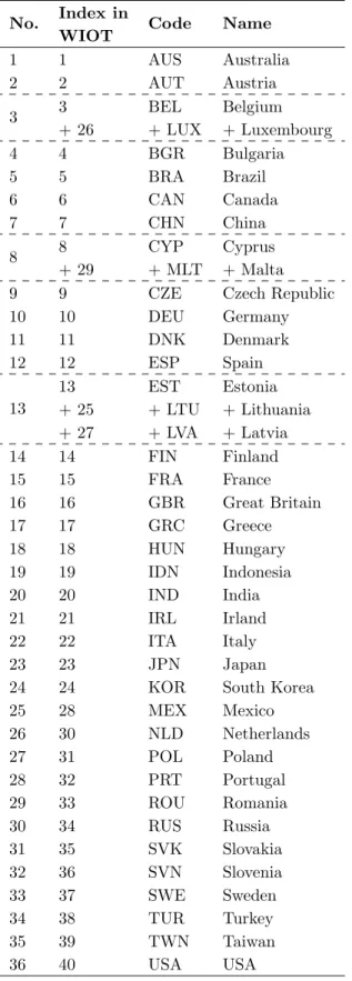
WIOTs of Release 2013 are provided as annual data from 1995 to 2011 covering 40 countries, including all 27 members of the EU (as of January 1, 2007) and 13 other major economies plus a rest of the world (RoW) region. As Timmer et al. (2015) point out, together the 40 countries cover more than 85 percent of world GDP in 2008 (at current exchange rates). Moreover, the data is provided for 35 industries, mostly at the two-digit ISIC Rev. 3 level or groups thereof, covering the overall economy. SEA dataset of Release 2013 comprises the same time span, countries (except RoW) and sectors as the WIOTs. However, for some countries data on some variables is only available until 2009. Variables of SEA that are expressed in nominal terms, like gross output at current prices or labor compensation, are denominated in national currencies.
4.1.2 Final data
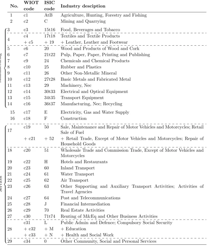
Before the concepts proposed in Sections 2 and 3 are applied, data from the WIOD is preprocessed. To make SEA data comparable across countries and consistent with the WIOT data, we convert all nominal values into US dollars. For that purpose, we use exchange rates provided as a complementary table for the WIOD Release 2013. The same exchange rates have been applied by the authors of the WIOD project to express the quantities in WIOTs for all countries in US dollars. To avoid problems that may arise in the calculations due to data issues, in the next step we aggregate some sectors and countries. Further, we eliminate two sectors: “Coke, Refined Petroleum and Nuclear Fuel” (ISIC code: 24) and “Private Households with Employed Persons” (ISIC code: P). The same sector/country transformation is applied to both the WIOTs and SEA data.
Lastly, we exclude RoW from WIOTs as no data on this region is available in SEA. A more detailed explanation of the reasons for data transformation as well as information on sectors and countries that have been aggregated can be found in Appendix C.4. After the initial data transformation the dataset covers 36 countries and 29 sectors, see Tables C.1 and C.2 in the appendix for more details.13
4.1.3 Computational details
Since the focus of our study lies on the assessment of a country’s competition, in the empirical application we will resort to the concepts of domestic EULC and EREER, where the latter, as has been explained in Section 3, is defined in terms of relativedomestic
EULC. Throughout this section, we will write EULC as a shorthand when referring to
domestic EULC. It should not be confused with the notion of EULC that also comprise the foreign contributions.
Sectoral EULC are calculated as follows. First, sectoral standard ULC are obtained as the ratio of sectoral labor costs and sectoral value added, where labor costs are represented by the variable labor compensation (labeled “LAB”) from the SEA dataset and value added is taken from the WIOTs.14 Since both variables are given in nominal terms, the
resulting ULC are interpreted as real ULC. Whereas for many countries data on labor compensation is available until 2011, for some countries the sample already ends in 2009. For the analysis to be consistent, the data must refer to the same time span for all countries. Since ULC show extreme behavior around 2008–2009 due to the economic and financial crisis, we restrict the analysis to end in 2007 instead of 2009.
The next component needed to obtain EULC are sectoral weights given by the ma-trix Ωe defined in eq. (14). All quantities used for the calculation of the weights are
13Throughout this section, we will additionally provide the WIOT code (number following the letter
“c”) while referring to a particular sector.
14SEA also contains another variable representing labor costs—compensation per employee (labeled
“COMP”). However, in our view labor compensation is a more suitable measure as it also contains compensation of self-employed in addition to compensation of employees. Since labor and capital com-pensation sum up to value added, sectoral ULC computed with the labor comcom-pensation variable also represent the labor share in a sector.
retrieved from the WIOTs: value added, gross output and the matrix of intermediate sales.
As regards sectoral EREERs, the computations involve EULC from the previous step and value-added bilateral weights based on domestic value added in bilateral gross ex-ports that is absorbed abroad, see eq. (28). For the computation of these EREER weights we utilize quantities taken from the WIOTs: value added, gross output, matrix of inter-mediate sales and final demand. For comparison purposes, we also calculate EREERs with gross export weights instead of value-added weights. In addition, we calculate two standard REER measures using standard ULC as a deflator which differ depending on whether value-added or gross export weights are used. For all four types of REER we resort to overall trade weights with double export weights that are given in eq. (30).
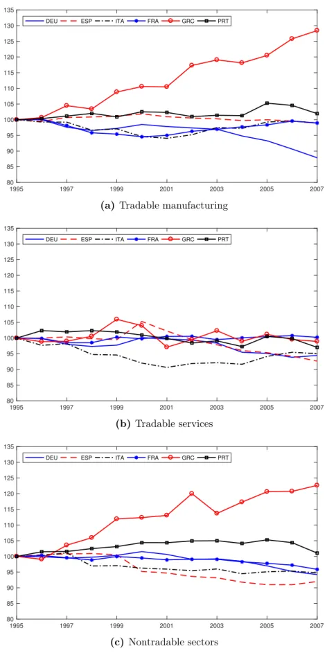
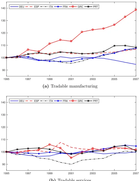
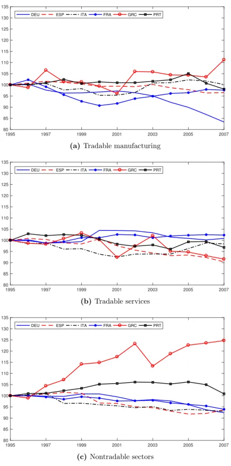
The subsequent part of this section sheds new light on changes in international com-petitiveness at the sectoral level for Germany, and compares the computed measures for German sectors with the corresponding ones in other selected euro area countries—Spain, Italy, France, Greece and Portugal. It is to be noted that the trading partner countries in the computations of different REER measures for Germany as well as each of the selected other euro area countries are always the other 35 countries from our sample. Hence, changes in the REER measure for a country always reflect changes in “overall” cost competitiveness, and not only changes in competitiveness relative to the other five countries from the comparison group. All ULC and REER series in the next subsection are depicted as index series, which, for each of the measures, are obtained by dividing the value in a particular year by the value in the first year in the sample (1995).
The presentation of stylized facts is facilitated by first considering sectoral aggregates instead of single sectors. Sectoral aggregates are constructed as follows. An industry in a particular country is classified as a nontradable (tradable) sector if gross exports of this industry lie below (above) the 25th percentile of the gross exports’ distribution in this country in 1995. Tradable sectors belonging to manufacturing (services) are assigned to the subgroup tradable manufacturing (tradable services). The three sectoral aggregates considered in our analysis therefore are: nontradable sectors, tradable manufacturing and tradable services.
Applying the “25th-percentile rule” yields sectoral aggregates that may vary from country to country with respect to their sectoral composition. However, for a meaningful comparison of one country with other countries the same sector classification should be chosen. Since the focus of our empirical application is on the international cost com-petitiveness of German sectors, we assign sectors in the comparison countries to the sectoral aggregates—nontradable sectors, tradable manufacturing and tradable services— according to the German classification that is presented in Table E.3 in Appendix E. Note that the German sector c1: “Agriculture, Hunting, Forestry and Fishing” is a tradable sector that belongs neither to tradable manufacturing nor to tradable services. It is there-fore subsumed under the group “other sectors” in Table E.3. This group is not explicitly examined, except in a few cases where information for this subgroup is useful for the interpretation of the results for the three main sectoral aggregates.
We calculate EULC for the three sectoral aggregates, as explained in Section 2.3, using sectoral standard ULC and the matrixΩe. To obtain EREERs for the sectoral aggregates, we proceed as outlined in Section 3.3 by employing EULC computed in the previous step as well as bilateral value-added weights for nontradable sectors, tradable manufacturing and tradable services.
4.2
Stylized facts for Germany
4.2.1 Results for sectoral aggregates
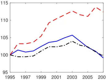
To get a first intuition about the costs evolution in different sectors in an economy, it seems natural to start with a look at the evolution of wages. Figure 1 shows the development of real hourly wages in Germany for the three sectoral aggregates (tradable manufacturing, tradable services and nontradable sectors) from 1995 to 2007.15 Real wages in tradable
15Real hourly wages in each of the aggregates are computed by deflating nominal hourly wages by
the consumer prices index (CPI) in the total economy. Source of the CPI is the GENESIS database of the German Federal Statistical Office (https://www-genesis.destatis.de/genesis/online). Nominal hourly wages are obtained by dividing labor compensation by the number of hours worked (total hours worked by persons engaged) for the respective sectoral aggregate. Labor compensation and hours worked at the level of individual sectors are retrieved from the SEA database (labels “LAB” and “H EMP”,
manufacturing increased by about 13 percent over this period which is in stark contrast to the wage developments in the nontradable sectors and in tradable services for which real wages showed only a slight increase until 2003 and declined afterwards. This decline may be related to the Hartz reforms that started in 2003 and led to a sizable increase in low-wage employment, especially in the nontradable sectors. However, it would be premature to conclude that manufacturing has profited via intermediate-good linkages from stagnating real wages in other domestic sectors, since sectoral cost developments depend on the change in wages relative to changes in productivity, i.e. on ULC.
1995 1997 1999 2001 2003 2005 2007 95 100 105 110 115
Figure 1: Real hourly wages in three German sectoral aggregates; red dashed line: tradable manufac-turing, black dash-dot line: tradable services, blue solid line: nontradable sectors.
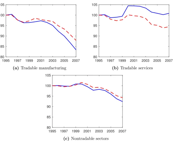
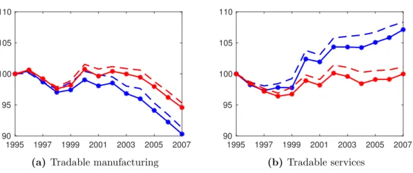
The blue solid lines in Figure 2 depict the development of standard ULC for the three sectoral aggregates. From 1995 to 2007, standard ULC declined by 16.6 percent in tradable manufacturing, stayed more or less constant in tradable services, and declined by 7.6 percent in nontradable sectors. Given the real wage developments discussed previously, these ULC developments are quite remarkable and point to a strong increase in labor productivity in tradable manufacturing that overcompensated the real wage increase, as opposed to only a slight increase in labor productivity in nontradable sectors and a roughly constant labor productivity in tradable services. Since standard ULC developed less favorably in nontradable sectors and tradable services in comparison to tradable
respectively) after the initial data preparation (see Section 4.1.2) and then aggregated to the level of nontradable sectors, tradable manufacturing and tradable services.
1995 1997 1999 2001 2003 2005 2007 80 85 90 95 100 105
(a) Tradable manufacturing
1995 1997 1999 2001 2003 2005 2007 80 85 90 95 100 105 (b) Tradable services 1995 1997 1999 2001 2003 2005 2007 80 85 90 95 100 105 (c) Nontradable sectors
Figure 2: Standard ULC and embodied ULC (EULC) in three German sectoral aggregates; blue solid line: standard ULC, red dashed line: EULC
manufacturing, EULC (depicted by the red dashed line) in tradable manufacturing showed a smaller decline than standard ULC. In contrast, especially tradable services profited from the ULC decline in the other two sectoral aggregates.
To trace the sources for the differences between standard ULC and EULC in the sec-toral aggregates, it may be informative to look at the individual sectors contributing to the sectoral aggregates. Table E.3 in the appendix reports the annual and total growth rate of standard ULC for all sectors and the respective value-added contribution to the final good in the three sectoral aggregates. For instance, for all sectors in tradable man-ufacturing, with the exception of sector c3: “Food, Beverages and Tobacco”, standard ULC declined from 1995 to 2007. However, it must be taken into account that tradable services and nontradable sectors also contributed with their value added to tradable man-ufacturing. The most prominent example is the service sector c30: “Renting of Machinery & Equipment and Other Business Activities” which contributed with 9.4 percent to trad-able manufacturing and experienced a 29.1 percent increase of standard ULC, thereby dampening the decline of EULC in tradable manufacturing.
In contrast, nontradable sectors and tradable manufacturing helped to increase com-petitiveness in tradable services. For example, the nontradable sector c17: “Electricity, Gas and Water Supply” contributed with 0.5 percent to final goods production in tradable services and experienced a 27.9 percent decline in ULC. Both, the manufacturing sectors c12: “Electrical and optical equipment” and c14: “Manufacturing, Nec; Recycling” had ULC declines of more than twenty percent over the sample period and contributed about 0.4 percent to tradable services. Even though the contribution of individual sectors from tradable manufacturing and nontradable sectors to tradable services is small, the total effect is large enough to bring about a 5.6 percent decline in EULC for tradable ser-vices from 1995 to 2007, whereas standard ULC increased by 0.9 percent over the sample period.
These results are at odds with one of the conclusions in the influential study of Dustmann et al. (2014) who, as mentioned in the introduction, claim that tradable manu-facturing in Germany has increased competitiveness by using intermediate inputs from tradable services. This contradicting evidence requires some further elaborations.
First, it is important to note that the authors construct the same three sectoral ag-gregates by applying the same “25th-percentile rule” as in our paper (see Section 4.1.3). Despite other data sources, their reported standard ULC in the time span 1995–2007 (see “unit labor costs: value added” in Figure 4 of Dustmann et al., 2014) strongly resemble the standard ULC depicted in Figure 2 of this paper. In other words, the benchmark ULC in Dustmann et al. (2014) and in our paper are almost in line. The conclusion of the authors about the increased competitiveness in tradable manufacturing and the reasons behind this development is thus not a consequence of a different benchmark. It results from the application of an ULC measure based on gross output that, according to the authors, should take account of the inter-sectoral linkages and is considered in their paper as an alternative to the benchmark ULC. However, this measure yields ULC in tradable manufacturing (see “unit labor costs: end products” in Figure 4 of Dustmann et al., 2014) which lie below standard ULC. This outcome is explained by the authors mainly by the fact that manufacturing bought inputs from sectors that experienced a decrease in wages, especially from tradable services. Though it is true that wages in nontradable sectors and tradable services fell strongly after 2003 compared to tradable manufacturing, we would like to point out that it is not correct to base arguments on changes in competitiveness on these wages developments, since changes in productivity are also decisive. Hence, it is developments in ULC and not in wages which matter.
It has been shown above that ULC in tradable services and nontradable sectors de-clined less strongly relatively to manufacturing. Therefore, since manufacturing drew on inputs from other domestic sector aggregates, this must reduce the increase in competi-tiveness in tradable manufacturing. ULC that adequately take account of inter-sectoral linkages must show a smaller and not a stronger decline.16 Our EULC concept with a
Leontief-type model as its foundation produces such a result as it captures the impact of other sectors’ cost developments for the competitiveness of a sector in a consistent manner. A further aspect which is not taken into account in the competitiveness analysis of Dustmann et al. (2014) but which is crucial in this context is that the evidence for the
16In Appendix D.3, we explain in more detail why, in our view, “unit labor costs: end products”—the