DOI 10.1007/s10618-012-0273-y
Diverse subgroup set discovery
Matthijs van Leeuwen · Arno Knobbe
Received: 31 October 2011 / Accepted: 21 May 2012 / Published online: 10 June 2012 © The Author(s) 2012. This article is published with open access at Springerlink.com
Abstract Large data is challenging for most existing discovery algorithms, for sev-eral reasons. First of all, such data leads to enormous hypothesis spaces, making exhaustive search infeasible. Second, many variants of essentially the same pattern exist, due to (numeric) attributes of high cardinality, correlated attributes, and so on. This causes top-k mining algorithms to return highly redundant result sets, while ignoring many potentially interesting results. These problems are particularly appar-ent with subgroup discovery (SD) and its generalisation, exceptional model mining. To address this, we introduce subgroup set discovery: one should not consider indi-vidual subgroups, but sets of subgroups. We consider three degrees of redundancy, and propose corresponding heuristic selection strategies in order to eliminate redun-dancy. By incorporating these (generic) subgroup selection methods in a beam search, the aim is to improve the balance between exploration and exploitation. The pro-posed algorithm, dubbedDSSD for diverse subgroup set discovery, is experimentally
Responsible editor: Dimitrios Gunopulos, Donato Malerba, Michalis Vazirgiannis.
The research described in this paper builds upon and extends the work appearing in ECML PKDD’11
(van Leeuwen and Knobbe 2011).
M. van Leeuwen (
B
)Machine Learning, Department of Computer Science, Katholieke Universiteit Leuven, Leuven, Belgium
e-mail: [email protected] M. van Leeuwen
Algorithmic Data Analysis, Department of Information and Computer Sciences, Faculty of Science, Universiteit Utrecht, Utrecht, The Netherlands
A. Knobbe
Leiden Institute of Advanced Computer Science, Universiteit Leiden, Leiden, The Netherlands e-mail: [email protected]
evaluated and compared to existing approaches. For this, a variety of target types with corresponding datasets and quality measures is used. The subgroup sets that are discovered by the competing methods are evaluated primarily on the following three criteria: (1) diversity in the subgroup covers (exploration), (2) the maximum quality found (exploitation), and (3) runtime. The results show thatDSSD outperforms each traditional SD method on all or a (non-empty) subset of these criteria, depending on the specific setting. The more complex the task, the larger the benefit of using our diverse heuristic search turns out to be.
Keywords Subgroup set discovery·Exceptional model mining·Pattern selection· Heuristic search·Diversity
1 Introduction
The field of subgroup discovery (SD) is concerned with the discovery of subsets of the data, where the target attribute(s) show an interesting difference in distribution, compared to that of the entire dataset. As such, the field encompasses all forms of discovery of local patterns in an exploratory, supervised setting. The typical definition of a SD task involves finding all subgroups that fit certain user-specified inductive constraints, and show a sufficiently high interestingness according to some chosen quality measure. SD algorithms have been developed for a large variety of data types, ranging from simple discrete attribute-value data, to very large and complex datasets of numeric and relational nature (see Sect.8for some examples). Especially in the case of these more challenging datasets, the traditional emphasis on completeness of the result is problematic.
In this paper, we address two important problems relating to the analysis of large and complex data. First, manual inspection of the resulting subgroup set is often ham-pered by the many subgroups reported and the high levels of redundancy in this result set. Second, when dealing with challenging data, for example when many high-car-dinality attributes are involved, the hypothesis space becomes extremely large, and the whole discovery process becomes overly time-consuming. It turns out that both problems revolve around the notion of diversity in sets of subgroups. For the result set redundancy problem, achieving more diversity will clearly address the many very similar subgroups. For the large search space problem, we will argue that heuristic search becomes a necessity, and demonstrate that retaining diversity during the search process is of paramount importance.
In the majority of discovery algorithms, including those for SD (Klösgen 1996; Wrobel 1997), it is assumed that complete solutions to a particular discovery task are required, and thus some form of exhaustive search is employed. In order to obtain effi-ciency, these algorithms typically rely on top-down search combined with considerable pruning, exploiting either anti-monotonicity of the quality measure (e.g. frequency), or so-called optimistic estimates of the maximally attainable quality at every point in the search space (Grosskreutz et al 2008). With small datasets and simple tasks, these tricks work well and give complete solutions in reasonable time. However, on large and complex datasets, exhaustive approaches simply become infeasible, even
when considerable pruning can be achieved. Additionally, we consider exceptional model mining (EMM) (Leman et al 2008;Duivesteijn et al 2010;van Leeuwen 2010), which allows multiple target attributes and complex models to be used for measuring quality. With EMM in particular, we are often dealing with quality measures that are not monotonic, and for which no optimistic estimates are available.
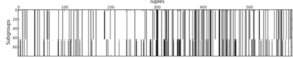
Apart from the computational concerns with discovery in large datasets, one also needs to consider the practicality of complete solutions in terms of the size of the output. Even when using condensed representations (Mannila and Toivonen 1996;Pasquier et al 1999) or some form of pattern set selection (Bringmann and Zimmermann 2007; Knobbe and Ho 2006b;Peng et al 2005) as a post-processing step, the end result may still be unrealistically large, and represent tiny details of the data overly specifically. The experienced user of discovery algorithms will recognise the large level of redun-dancy that is common in the final pattern set. This redunredun-dancy is often the result of dependencies between the (non-target) attributes, which lead to large numbers of vari-ations of a particular finding. Note that large result sets are problematic even in top-k approaches. Large result sets are obviously not a problem in top-1 approaches, but they are when k≥2, as the mentioned dependencies will lead to the top of the pattern list being populated with different variations on the same theme, and alternative patterns dropping out of the top-k. This problem is aptly illustrated by Fig.1, which shows that the top-100 subgroups obtained on the Emotions dataset (see Sect.7on experiments) cover almost exactly the same tuples.
The obvious alternative to exhaustive search, and the one we consider in this paper, is heuristic search: employ educated guesses to consider only that fraction of the search space that is likely to contain the patterns of interest. When performing heuristic search, it is essential to achieve a good balance between exploitation and exploration. In other words, to focus and extend on promising areas in the search space, while leaving room for several alternative lines of search. In this work, we will implement this balance by means of beam search, which provides a good mixture between parallel search (exploration) and hill-climbing (exploitation). We will experiment with different vari-ations of achieving diversity in the beam, that is, the current list of candidates to be extended. Due to the above-mentioned risk of redundancy with top-k selection, the level of exploration within a beam can become limited, which will adversely affect the quality of the end result. Inspiration for selecting a diverse collection of patterns for the beam at each search level will come from pattern set selection techniques (Bringmann and Zimmermann 2007;Knobbe and Ho 2006b;Peng et al 2005), which were originally designed for post-processing the end-result of discovery algorithms.
Fig. 1 Redundancy in top-k EMM. Shown are the covers (in black) of the top-100 subgroups obtained
1.1 Redundancy in subgroup sets
To better appreciate the reasons behind redundancy in subgroups sets, consider an example from practice that relates to car accidents. Assume the car accidents are described by a number of attributes, including the following:1
fatalities positive integer
nature {fatal, injured, damage only} time {day, night}
cost positive real
Although the attributes fatalities and nature are not perfectly correlated, they do convey some mutual information, and will lead to multiple similar patterns. This redundancy is already visible after a first analysis of depth-1 subgroups, where the following ranking of subgroups is obtained:
1. fatalities ≥1 2. nature=fatal
3. fatalities ≥2
4. nature=damage only
5. time=night
. . . .
Assuming a beam widthw=4, only the first four subgroups will be used to build candidates for the next level, and as a result, the subgroup time=night (and all lower
ranking ones) will be ignored. On the next level, the ranking could be as follows: 1. fatalities ≥1∧nature=fatal
2. fatalities ≥1∧nature=damage only
3. fatalities ≥1∧fatalities ≥2 4. nature=fatal∧cost≥123.4
. . . .
Note how the top of the ranking has become saturated with variations on the theme
fatalities ≥1. For example, the condition time=night was not considered for the
sec-ond level, due to the limited beam width, and any potentially interesting combinations with for example cost where never investigated.
Note that although our example suggests otherwise, redundancy in subgroup col-lections need not just be the result of strict functional dependencies in the data (such as
fatalities≥1→nature= fatal), but can also be due to dependencies of more statistical nature. As such, concepts such as condensed representations (Mannila and Toivonen 1996;Pasquier et al 1999) will not suffice to achieve diversity in the intermediate and final subgroups sets.
Such causes of redundancy, both in the search beam and the final result set, are par-ticularly frequent in large and complex datasets. The most obvious form of complexity in datasets is large numbers of attributes. As the hypothesis space grows exponentially
1 The target attribute is not relevant here, but could for example convey whether the accident resulted in
with the number of attributes, exhaustive search becomes prohibitively time-consum-ing. A further contributing factor in the size of the hypothesis space, one that is not relevant in for example frequent itemset mining, is the cardinality of attributes. As nominal attributes can assume more than two values, testing for equality will produce multiple possible refinements per candidate subgroup. The cardinality of an attribute is of particular relevance in the case of numeric attributes, as in theory, the cardinality of the attribute could be as high as the number of tuples in the dataset (e.g. think of the cost of a car accident). Although in our SD implementation, we do not test for every conceivable threshold in the continuous domain—we use a form of dynamic discretisation—numeric attributes are still a major factor in the run times. Finally, when the data in question no longer concerns attribute-value data, but more complex representations, such as relational (Knobbe 2006) or graphical (Yan and Han 2002), the search space becomes even larger.
1.2 Contributions and roadmap
This paper is a significant extension of our recent paper (van Leeuwen and Knobbe 2011) on non-redundant generalised subgroup discovery (GSD). Although the main message of the paper is unchanged, it encompasses important novel contributions. First of all, the beam selection methods are now presented as generic subgroup
selec-tion methods and three addiselec-tional selecselec-tion strategies that dynamically determine the
number of subgroups to be selected are introduced. Second, the complete algorithm is separately introduced, explained and dubbed DSSD, which stands for diverse subgroup set discovery.
Third, the experiments now include a much wider range of datasets and com-parisons to sequential and weighted covering methods, showing in more detail the benefits of our techniques on complex data. Apart from the previous binary and multi-target (EMM) settings, the experiments also include discovery with either nominal or numeric targets. These experiments demonstrate the use of diverse SD in a multi-class and regression setting, respectively. Additionally, the collection of quality measures considered has been extended, most notably for multi-class and continuous targets. Finally, throughout the paper, we have extended the descriptions in order to clarify details and provide more background, for example in the related work section.
In Sect.2, we will first formalise both SD and EMM, after which we will recap the commonly used search techniques, including the standard beam search algorithm. Section3presents the quality measures that will be used in the experiments. We will then introduce the notion of subgroup set discovery in Sect.4, and argue that it is bet-ter to mine subgroup sets rather than individual subgroups, to ensure diversity. This leads to the non-redundant GSD problem statement. We will show that redundancy in subgroup sets can be formalised in (at least) three different ways, each subsequent def-inition being stricter than its predecessor. Each of these three degrees of redundancy is used as principle for two subgroup selection strategies in Sect.5. The complete
DSSD algorithm is presented in Sect.6, and includes a method for pruning individ-ual subgroup descriptions and a detailed description of the refinement operator. After that, we continue with an extensive empirical evaluation in Sect.7. We round up with related work and conclusions in Sects.8and9.
2 Preliminaries 2.1 SD and EMM
We assume that the tuples to be analysed are described by a set of attributes A, which consists of k description attributes D and l model(or target)attributes M (k≥1 and
l ≥ 1). In other words, we assume a supervised setting, with at least a single target attribute M1(in the case of classical SD), but possibly multiple attributes M1, . . . ,Ml
(in the case of EMM). Each attribute Di (resp. Mi) has a domain of possible values
Dom(Di)(resp. Dom(Mi)). Our datasetSis now a bag of tuples t over the set of attri-butes A= {D1, . . . ,Dk,M1, . . . ,Ml}. We use xDresp. xM to denote the projection of x onto its description resp. model attributes, e.g. tD =πD(t)in case of a tuple, or SM =π
M(S)in case of a bag of tuples. Equivalently for individual attributes, e.g. SMi =π
Mi(S).
Arguably the most important concept in this paper is the subgroup, which consists of a description and corresponding cover.
Definition 1 (Subgroup cover) A subgroup (cover) is a bag of tuples G ⊆Sand|G|
denotes its size, also called subgroup size or coverage.
Definition 2 (Subgroup description) A subgroup description is an indicator function
s, as a function of description attributes D. That is, it is a function s :(Dom(D1)×
. . .×Dom(Dk))→ {0,1}, and its corresponding subgroup cover is Gs = {t ∈ S | s(tD)=1}.
As is usual, in this paper a subgroup description is a pattern, consisting of a con-junction of conditions on the description attributes, e.g. Dx = tr ue∧ Dy ≤ 3.14.
Such a pattern implies an indicator function as just defined.
Given a subgroup G, we would like to know how interesting it is, looking only at its model (or target) data GM. We quantify this with a quality measure.
Definition 3 (Quality measure) A quality measure is a functionϕ : GM →Rthat assigns a numeric value to a subgroup GM ⊆ SM, withGM the set of all possible subsets ofSM.
SD and EMM The above definitions allow us to define the two main variations of
data mining tasks that feature in this paper: SD and EMM. As mentioned, in SD we consider datasets where only a single model attribute M1(the target) exists. We are interested in finding the top-ranking subgroups according to a quality measureϕthat determines the level of interestingness in terms of unusual distribution of the target attribute M1:
Problem 1 (Top-k SD) Suppose we are given a datasetSwith l=1, a quality measure
ϕand a number k. The task is to find the k top-ranking subgroupsGk with respect to
ϕ.
EMM is a generalisation of the well-known SD paradigm, where the single target attribute is replaced by a collection of model attributes (Leman et al 2008). Just like in
SD, EMM is concerned with finding subgroups that show an unusual distribution of the model attributes. However, dependencies between these attributes may occur, and it is therefore desirable to consider the joint distribution over M1, . . . ,Ml. For this reason, modelling over GMis employed to compute a value forϕ. If the model induced
on GM is substantially different from the model induced onSM, quality is high and we call this an exceptional model. We can now formally state the EMM problem. Problem 2 (Top-k EMM) Suppose we are given a datasetS, a quality measureϕand a number k. The task is to find the k top-ranking subgroupsGkwith respect toϕ. 2.2 Subgroup search
To find high-quality subgroups, the usual choice is a top-down search strategy. The search space is traversed by starting with simple descriptions and refining these along the way, from general to specific. For this a refinement operator that specialises sub-group descriptions is needed. For example, given the empty subsub-group description, the refinement operator generates all descriptions consisting of a single condition. Given any subgroup description X , consisting of|X| conditions, it generates all allowed descriptions of size|X+1|containing X . These are the refinements of X .
Algorithms for SD commonly use the following two parameters to restrict the search space. A minimum coverage threshold (mincov) is used to ensure that a subgroup covers at least a certain number of tuples. A maximum depth (maxdepth) parameter imposes a maximum on the number of conditions a description may contain. The term depth refers to the shape of the search space, which can be regarded a tree.
Exhaustive search When exhaustive search is possible, depth-first search is
com-monly used. This is often the case for moderately sized nominal datasets with a single (binary) target. Whenever possible, (anti-)monotone properties of the quality measure are used to prune parts of the search space, a technique that is also commonly used in frequent pattern mining (Han et al 2007).
When this is not possible, so-called optimistic estimates (Grosskreutz et al 2008) can be used to restrict the search space. An optimistic estimate function computes the highest possible quality that any refinement of a subgroup could give. If this upper bound is lower than the quality of the current kth subgroup, the current branch of the search space can be safely skipped without affecting the outcome of the algorithm. Depending on k, the dataset and the quality measure, this may lead to significant speed-ups.
Beam search When exhaustive search is not feasible, beam search (Lowerre 1976) is the widely accepted heuristic alternative. It is similar to exhaustive approaches in that it also uses a top-down strategy and a refinement operator, but it explores only part of the search space. For this, a level-wise search is performed, as bread-first search would do. However, on each level only a selection of all evaluated subgroups, i.e. the
beam, is used for refinement.
On each level a refinement operator generates subgroups for the next level from each individual subgroup in the beam. The initial candidate set is generated from the empty subgroup description. From all generated candidates on a particular level, the
During the search, a final result list is maintained, in which the overall top-k of all evaluated subgroups are kept.
Covering schemes To obtain diversity in rule induction and SD, so-called ‘covering’
schemes have been introduced. The well-known rule induction algorithm CN2 (Clark and Niblett 1989;Clark and Boswell 1991) introduced what we will call sequential
covering. Each round, the search procedure looks for the best rule, and subsequently
all training examples covered by this rule are removed. This procedure is repeated until a stopping criterion is met (e.g. all examples are covered). This way, an ordered rule set is induced. The authors also proposed a slightly different variant that generates an unordered rule set, but we do not consider that here because it can only be applied when there is a single nominal class label.
Inspired by CN2,Lavraˇc et al(2004) introduced an adaptation of CN2 for SD, aptly named CN2-SD. One of the modifications they proposed is a new covering scheme, to reflect the different goals of SD: in contrast to rule induction, it does not aim to maximise accuracy. Rather, it is meant to be exploratory and aims to give an overview of regions of the data that stand out with respect to the target. For this, it should be possible for subgroups to overlap, which is not possible with sequential covering.
To achieve this, weighted covering was proposed. Instead of completely removing all tuples in a subgroup cover, all tuples in the database with a positive class label are assigned a weight. All tuples start with a weight of 1, but when a tuple is covered its weight decreases. Furthermore, the weighted relative accuracy (WRAcc) quality measure is adapted to take these weights into account. For a tuple t that has been covered i times, its weightw(t,i)can be computed in two ways. With multiplicative weights:w(t,i)=γi (for a given parameter 0< γ <1), or with additive weights:
w(t,i)= i+11.
We will empirically compare our methods to sequential covering and (a more generic variation on) multiplicative weighted covering in Sect.7.
Exception maximisation description minimisation (EMDM) Invan Leeuwen(2010) we introduced an alternative heuristic algorithm for EMM called EMDM. It is based on the observation that in EMM, both the description and the model data can be exploited to guide the search. Starting from a set of candidates that are likely to be of reasonable quality, subgroups are improved in an iterative manner. The first step, called exception maximisation, modifies the cover of a subgroup such that its quality is maximised. Next, the second step, called description minimisation, modifies the subgroup such that it can be succinctly described. These steps are alternately performed until a stable solution is found.
3 Quality measures
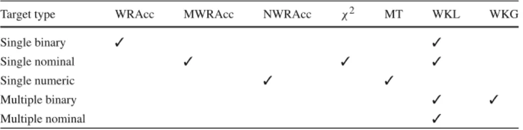
In this section we present the quality measures for individual subgroups that we will use in our experiments. Table1shows with which considered target types the quality measures can be used.
WRAcc WRAcc (Lavraˇc et al 2004) is a well-known SD quality measure for data-sets with a single binary target attribute. It consists of two components: (1) the (rela-tive) size of the subgroup and (2) the (rela(rela-tive) amount of positive examples that the
Table 1 Quality measures can only be used in combination with certain target types
Target type WRAcc MWRAcc NWRAcc χ2 MT WKL WKG
Single binary ✓ ✓
Single nominal ✓ ✓ ✓
Single numeric ✓ ✓
Multiple binary ✓ ✓
Multiple nominal ✓
All possible combinations are indicated with a checkmark
subgroup contains. Both of these positively contribute to a higher WRAcc. Let 1G (resp. 1S) denote the fraction of ones in the target attribute, within the subgroup (resp. entire dataset). The measure is then defined as
ϕWRAcc(G)=|G|
|S|(1
G−
1S).
Multi-class weighted relative accuracy (MWRAcc) Abudawood and Flach (2009) introduced several multi-class versions of WRAcc. We here adopt one, namely the one-vs-rest variant, because the experiments inAbudawood and Flach(2009) show that the differences between the different versions are marginal.
The principle of the one-vs-rest MWRAcc is simple: one can apply the regular ‘one-vs-one’ WRAcc measure by setting one of the target values to ‘positive’ and the rest to ‘negative’. By doing this procedure once for each possible target value and summing the qualities obtained this way, an overall quality can be computed. That is, the measure can be defined as
ϕMWRAcc(G)=
x∈Dom(M1)
|W R Accx(G)|,
where WRAccx(G)means thatϕW R Acc(G)is computed with x as positive class. Numeric weighted relative accuracy (NWRAcc) NWRAcc is a straightforward
trans-lation of regular WRAcc to the numeric case. LetμG (resp.μS) denote the mean of
all target values in the subgroup (resp. the entire dataset). The measure is then defined as
ϕWRAcc(G)= |G|
|S|(μG−μS).
Chi-squared (χ2) Theχ2test determines whether subgroup and class membership of a random tuple are statistically independent. Under the null hypothesis of assuming independence of columns and rows, the expected class frequencies can be computed from the marginals. Let xG (resp. xS) denote the fraction of tuples within the sub-group (resp. entire dataset) that have x as target value, for x∈Dom(M1). Then, for a subgroup G the expected frequency for a class x is||GS||xS. Theχ2statistic is the sum
of the squared differences between observed and expected frequencies divided by the expected frequencies, and can be written as
ϕχ2(G)= x∈Dom(M1) [|G|(xG−xS)]2 |G|xS + [|G|xG− |G|xS]2 (|S| − |G|)xS .
Mean test (MT) The MT was already introduced in the Explora system (Klösgen 1996). It quantifies the difference between the means of the target value in the subgroup and in the complete dataset and is defined as
ϕM T(G)=
|G|(μG−μS),
where μG andμS are defined as before. Note that subgroups with a high MT are relatively large subgroups with a relatively high mean. Subgroups with a mean that is very low compared to the overall distribution have a negative quality; the absolute value of the difference between the means could be taken if one is also interested in those subgroups.
Weighted Kullback–Leibler divergence (WKL) The KL divergence (Kullback and Leibler 1951) is an asymmetric measure of the difference between probability dis-tributions P and Q. It quantifies the number of extra bits which would be required to encode a sample from P using a code based on Q (‘wrong’ distribution) instead of using a code based on P (‘correct’ distribution).
For probability distributions P and Q of a discrete random variable, the KL diver-gence of Q from P is given as
KL(PQ)= x
P(x)log2
P(x) Q(x).
We previously introduced a measure based on the KL divergence invan Leeuwen (2010). We assume that each attribute-value in our database is an independently drawn sample from an underlying, independent discrete random variable, and empirically estimate the probability distribution for each attribute Mi. We denote the function
which derives such an empirical distribution byP, which is defined asˆ Pˆ(Mi =x)=
|{t∈S|tMi=x}|
|S| . We then defined KL exceptionality as the sum of KL divergences over
all individual attributes, from subgroup to database.
We here present an alternative that weighs quality by subgroup size, because this works better in combination with a level-wise search (without this weight, smaller subgroups tend to be of higher qualities). It is quite versatile as it can be easily used with a single or multiple binary model attributes, but also with nominal attributes. Definition 4 (WKL quality) Given a databaseSand subgroup G, define (independent)
Weighted KL quality as ϕWKL(GM)=|G| |S| l i=1 KL(Pˆ(GMi) ˆP(SMi))
WKL quality has the potential advantage that it treats all values equally; unlike
many quality measures for SD, 1s and 0s are considered symmetrically. When one is interested in deviating distributions, this is generally a desirable property. A downside of this quality measure is that all attributes are assumed to be completely independent. This assumption is likely to be violated when there are correlations between the model attributes.
Weighted Krimp gain (WKG) Invan Leeuwen(2010) we introduced a second mea-sure that, contrary to (Weighted) KL quality, does take associations between attributes into account. Another important difference is that it is asymmetric: it only considers 1s and neglects the 0s in the model data. Finally, it only works for binary data, although the generic idea (i.e. using compression to quantify differences between overall and subgroup distributions) could be applied to other types of data.
The WKG measure usesKrimp code tables (Vreeken et al 2011) as models. These are ordered lists of itemsets that have codes associated to them. A code table can be used to encode a binary database by replacing each occurrence of an itemset with its associated code.Krimp is a heuristic that approximates the optimal code table for a given database.
The basic principle is equivalent to that of WKL: a subgroup is interesting if it can be compressed (much) better by its own compressor, than by the compressor induced on the overall database. Similar to WKL quality, we here introduce a weighted alternative to take the size of the subgroup into account.
Definition 5 (WKG) LetDbe a binary database, G ⊆Da subgroup, and C TD and
C TG their respective optimal code tables. We define the WKG of group G fromD, denoted by WKG(GD), as
WKG(GD)=L(G|C TD)−L(G|C TG),
with L(G|C T)the size of G, in bits, encoded with code table C T . Given this, defining the quality measure is straightforward.
Definition 6 (WKG quality) LetS be a database and G ⊆ S a subgroup. Define
Weighted KG quality as
ϕWKG(GM)=WKG(GM SM).
4 Non-redundant GSD
As described in the introduction, redundancy can be a severe problem in discovery tasks such as SD and EMM. Many (slightly) different subgroup descriptions imply many (almost) equal subgroup covers that have (almost) equal similarity. This adversely affects the results of any search that aims to be complete, and top-k search in partic-ular. That is, the top-k is likely to contain many variations of the same theme, all of high quality, while clearly different subgroups are not presented to the user at all.
1. SD algorithms should never return the complete set of subgroups, but a condensed representation or ‘interesting’ selection thereof.
2. Subgroups should not be considered only individually, they should always be judged also on their joint merit.
That is, we should consider subgroup set discovery: discovery of a non-redundant set of high-quality subgroups. This aim is comparable to recent pattern set selection approaches (Bringmann and Zimmermann 2007;Knobbe and Ho 2006b;Peng et al 2005), although we focus on SD and EMM here. The revised task can be formulated as follows.
Problem 3 (Non-redundant GSD) Suppose we are given a datasetS, a quality mea-sureϕ and a number k. The task is to find a non-redundant setGof k high-quality subgroups.
The term GSD is used to emphasise that it encompasses both SD (single target) and EMM (multiple targets).
Given this task, the primary challenge is to define redundancy. Although it may be clear to a domain expert or data miner whether a (small) set of patterns contains redun-dancy or not, formalising redunredun-dancy is no trivial task. Several different approaches to formalising non-redundant pattern sets exist, e.g. using joint entropy (Cover and Thomas 2006;Knobbe and Ho 2006a;Bringmann and Zimmermann 2007), or min-imum description length (MDL) (Grünwald 2007; Vreeken et al 2011). Sequential and weighted covering, as described in Sect.2, also aim to increase diversity in the resulting subgroups.
However, very few of the existing methods can be straightforwardly applied to the task just mentioned, as they all make more specific assumptions about the task. For example, many methods assume that all description attributes are binary, and/or that there is a single binary target. We aim to develop methods that are specifically tailored to the GSD setting, without making any additional assumptions; they should work for any SD or EMM setting.
We consider three degrees of attaining diversity, which we consider equivalent to removing redundancy. The definitions in Sect.2show that a subgroup consists of a description and corresponding cover, which can be regarded as a subgroup’s intent resp. extent. This suggests that redundancy can be defined both intensionally and ex-tensionally. Further, in the EMM setting, we can also avail the models that are fitted on the subgroups, which suggests a third way to define redundancy. Hence, in a
non-redundant subgroup setG, all pairs Gi,Gj ∈G(with i = j ) should have substantially
different:
1. subgroup descriptions, or
2. subgroup covers, or
3. exceptional models. (Only in the case of EMM.)
Note that each subsequent degree is stricter than its predecessor. On the first, least restrictive degree, substantially different descriptions are allowed, ignoring any poten-tial similarity in the covers. The second degree of redundancy would also address sim-ilarity in the subgroup covers. The third degree of redundancy will consider subgroups
that are different in both description and cover, and will address their difference in terms of the associated models built on the model attributes M. As these models will typically somehow represent the data distribution of the model data, this definition of redundancy implicitly enforces subgroups to have different data distributions.
Without being subjective, it is impossible to state that one of these definitions of redundancy is absolutely better than the others. This depends much on the data and the requirements of the data miner or domain expert. Hence we do not choose one of the degrees, but proceed considering each of them. In Sect.5, each of the three degrees will be used as basic principle for two subgroup set selection methods.
4.1 Quantifying redundancy in subgroup covers
To be able to judge the effect of our methods and compare it to existing methods, such as the beam search described in Sect.2, it is imperative that we quantify redundancy. Here, we focus on measuring redundancy in the subgroup covers, i.e. it matches best with the second degree of redundancy.
In the work this paper builds upon (van Leeuwen and Knobbe 2011), we introduced a measure to quantify redundancy in the covers of subgroup sets. For this measure, dubbed cover redundancy (CR), we assume that a maximally diverse set of subgroups would uniformly cover all tuples in the dataset. Also, let the cover count of a tuple be the number of times it is covered by a subgroup in a subgroup set. Given this assump-tion and definiassump-tion, one can easily compute an expected cover count and measure how far each individual tuple’s cover count deviates from this. This results in the following definition:
Definition 7 (CR) Suppose we are given a datasetSand a set of subgroupsG. Define the cover count of a tuple t ∈Sas c(t,G)=G∈GsG(t). The expected cover count
ˆ
c of a random tuple t ∈Sis defined ascˆ=|S1|t∈Sc(t,G). Cover redundancy CR is now computed as:
CRS(G)= 1 |S| t∈S |c(t,G)− ˆc| ˆ c
The larger the CR is, the larger is the deviation from the uniform cover distribution. Because GSD aims to find only those parts of the data that stand out, this measure on itself does not tell us much; we cannot expect all tuples to be uniformly covered. However, CR is very useful when comparing different subgroup sets on the same dataset. If we have several subgroup sets of (roughly) the same size and for the same dataset, a lower CR indicates that fewer tuples are covered by more subgroups than expected, and thus the subgroup set is more diverse/less redundant.
In recent work on pattern set selection (Knobbe and Ho 2006a,b;Bringmann and Zimmermann 2007;Knobbe and Valkonet 2009), alternative measures for diversity in pattern sets were investigated. The most prominent of these, joint entropy, involves the information theoretical concept of entropy (Cover and Thomas 2006) over the binary features defined by each pattern (or subgroup, for that matter).
Definition 8 (Joint entropy) Suppose thatG= {G1, . . . ,Gk}is a set of subgroups, and
B=(b1, . . . ,bk)∈ {0,1}kis a tuple of binary values. Let p(sG1 =b1, . . . ,sGk =bk) denote the fraction of tuples t ∈S such that sG1(t)=b1∧. . .∧sGk(t)=bk. The
joint entropy ofGis defined as:
H(G)= −
B∈{0,1}k
p(sG1 =b1, . . . ,sGk =bk)log2p(sG1 =b1, . . . ,sGk =bk)
Note that H is measured in bits, and each subgroup provides at most 1 bit of infor-mation, such that H(G) ≤ |G|. Equality only occurs in the unlikely event that all subgroups cover half of the dataset, and each pair of subgroup covers is independent. Joint entropy has an inverse interpretation from CR: a high joint entropy between subgroups indicates low redundancy.
Informal comparison between the two measures shows that the measures are some-times highly correlated (although inverted), and somesome-times seem completely unrelated. This is unsurprising, as CR is computed from the cover count (the number of times a tuple is covered), whereas the joint entropy focuses on the counts of tuples with identical covers.
Example 1 As an example, the subgroup set visualised in Fig. 1has a high CR of 1.43. Its joint entropy equals 1.573 bits, which indicates that not more information is conveyed with these 100 subgroups than could be conveyed with just 2 subgroups (which would represent 2 bits in the ideal case). Clearly, this cover distribution is highly undesirable, and much lower values for CR and much higher values for H are preferred.
5 Diverse subgroup set selection
In this section, we show how the three degrees of redundancy that we identified previ-ously can be translated to subgroup selection strategies: procedures that select a small set of high-quality subgroups from a large number of candidate subgroups. The most naive strategy is to always select the k top ranking subgroups with respect to quality; this is the default used by the SD beam search outlined in Sect.2.2and we will refer to this as the TopK strategy.
Since we intend to incorporate the selection strategies within level-wise search, it is important that they are computationally not too heavy. Unfortunately, most pattern set selection criteria require considering all possible pattern sets to ensure that the global optimum is found. Because we will need to select subgroup sets from large numbers of subgroups multiple times in a single run, such exhaustive strategies are infeasible. Hence, we resort to greedy and heuristic methods, as is usual in pattern set selection (Bringmann and Zimmermann 2007;Knobbe and Ho 2006b;Peng et al 2005).
In the following, a pair of strategies will be introduced for each of the three degrees of redundancy, where one selects a fixed number k of subgroups and the other selects a variable number of subgroups. Each subsequent degree of redundancy is stricter than its predecessor, but also results in computationally more demanding procedures. This
offers the data miner the opportunity to trade-off diversity with computation time. The aim of the variable-size strategies is to select fewer subgroups than their fixed-size counterparts, providing fast alternatives that still give reasonable results.
5.1 Description-based subgroup selection
Here we select subgroups purely on the basis of their descriptions, not considering their corresponding covers whatsoever. This is fast and potentially eliminates quite some redundant subgroups.
Fixed-size description-based selection (Desc(k)) This strategy greedily selects
sub-groups by comparing each candidate to the subsub-groups already selected. If there is a selected subgroup that has (1) equal quality and (2) the same conditions except for one, the candidate is skipped.
The procedure to achieve this is as follows. Order all candidate subgroups descend-ing on quality and consider them one by one until the desired number of subgroups k is reached. For each considered subgroup G∈Cands, discard it if its quality and all
but one conditions are equal to that of any G ∈Sel, otherwise include it in the
selec-tion. Time complexity for selecting a subgroup set isO(|Cands| ·log(|Cands|)+
|Cands|·maxlen)(where maxlen is the maximum number of conditions any
descrip-tion contains).
Variable-size description-based selection (VarDesc(c,l)) An alternative way to
achieve diversity is to allow each description attribute to occur only c times in a con-dition in a subgroup set. Because the number of occurrences of an attribute depends on the number of conditions per description, each attribute is allowed to occur cl times, where l is the (maximum) length of the descriptions in the candidate set. The beam width now depends on the number of description attributes|D|, c and l. This effectively results in a (more or less) static beam width per experiment.
Order all candidate subgroups descending on quality and consider them one by one. For each considered subgroup G∈Cands, check whether any of its conditions
specifies an attribute that has already been used cl times. If so, discard the candidate, otherwise add it to selection Sel and update the attribute usage counts. Stop when all attributes occur cl times in the selection or when no more candidates are available. Time complexity for subgroup selection isO(|Cands| ·log(|Cands|)).
5.2 Cover-based subgroup selection
Taking subgroup covers into account is computationally more intensive than consid-ering only the descriptions, but also results in more diversity.
Fixed-size cover-based selection (Cover(k)) A score based on multiplicative weighted
covering (Lavraˇc et al 2004) is used to weigh the quality of each subgroup, aiming to minimise the overlap between the selected subgroups. This score is defined as
(G,Sel)= 1
|G|
t∈G
where α ∈ 0,1]is the weight parameter. The less often tuples in subgroup G are already covered by subgroups in the selection, the larger the score. If the cover con-tains only previously uncovered tuples,(G,Sel)=1.
In k iterations, k subgroups are selected. In each iteration, the subgroup that maxi-mises(G,Sel)·ϕ(G)is selected. The first selected subgroup is always the one with the highest quality, since the selection is empty and(G,Sel)=1 for all G. After that, the-scores for the remaining Cands are updated each iteration. Complexity is
O(k· |Cands| · |S|).
Variable-size cover-based selection (VarCover( f )) This selection procedure is
equiva-lent to the fixed-size version, except for the stopping criterion. Subgroups are iteratively selected until no candidate subgroup meets the minimum scoreδspecified by param-eter f . The minimum score is defined as a fraction of the quality of the top-ranking candidate, i.e.δ= f·maxG∈Candsϕ(G). Selection stops when there is no G∈Cands
for which(G,Sel)·ϕ(G)≥δ. 5.3 Compression-based beam selection
To be able to do model-based beam selection, a (dis)similarity measure on models is required. For this purpose, we focus on the models used by the WKL and WKG quality measures. These measures have in common that they rely on compression; they assume a coding scheme and the induced models can therefore be regarded as
compressors.
In case of WKG, the compressor is the code table induced byKrimp. In case of
WKL, the compressor replaces each attribute-value x by a code of optimal length L(x)
based on its marginal probability, i.e.
L(x)= −log2(Pˆ(Mi =x)).
Adopting the MDL principle (Grünwald 2007), we argue that the best set of compres-sors is that set that together compresses the dataset best. Selecting a set of comprescompres-sors is equivalent to selecting a set of subgroups, since each subgroup has exactly one corre-sponding compressor. Since exhaustive search is infeasible, we propose the following heuristic.
1. We start with the ‘base’ compressor that is induced on the entire dataset, denoted
CS. Each t ∈ S is compressed with this compressor, resulting in encoded size L(S|CS).
2. Next, we iteratively search for the subgroup that improves overall compression most, relative to the compression provided by the subgroups already selected. That is, the first selected subgroup is always the top-ranked one, since its compressor
C1gives the largest gain with respect to L(S |CS).
3. Each transaction is compressed by the last picked subgroup that covers it, and by
CSif it is not yet covered by any. So, after the first round, part of the transactions are encoded by CS, others by C1.
4. Assuming this encoding scheme, select that subgroup G ∈ Cands\ {C1, . . .}
5. Repeat step 4 until some stopping criterion is reached.
To perform this selection strategy, all compressors belonging to the subgroups of a certain level are required. If these can be kept in memory, the complexity of the selection scheme isO(k· |Cands| · |S| · |M|), where k is the (maximum) number of subgroups to be selected and|M|is the number of model attributes. However, keeping all compressors in memory may not be possible. They could then be either cached on disk or reconstructed on demand, but both approaches severely impact runtimes.
Fixed-size compression-based selection (Compress(k)) Using the heuristic outlined
above, a fixed-size selection scheme is obtained by choosing an appropriate stopping criterion: stop when the selection contains k subgroups.
Variable-size compression-based selection (VarCompress) MDL provides us a
nat-ural and parameter-free stopping criterion for the variable-size scheme. That is, we should stop when compression cannot be improved, meaning that we should stop when
L(S|CS,C1, . . . )−L(S|CS,C1, . . . ,G)≤0.
6 DSSD: diverse beam search for non-redundant discovery In this section we present the completeDSSD algorithm.
6.1 TheDSSD algorithm
The six generic subgroup set selection strategies presented in the previous section were primarily designed to improve the standard SD beam search. Instead of simply choosing the—potentially highly redundant—top-k subgroups for the beam, one of the six more advanced selection strategies is used.
The overall subgroup set discovery algorithm we propose, shown in Algorithm1, consists of three phases. First, a beam search is performed to mine j subgroups (lines 1–12), using any of the proposed subgroup selection strategies to select the beam on each level (10). The refinement operator used on line 5 is described in more detail in the next subsection. In the second phase, each of the j resulting subgroups is individ-ually improved using dominance pruning (see Sect.6.3), and syntactically equivalent subgroups are removed (13–16). As the final result set potentially still suffers from the redundancy problems of top-k-selection (line 8), in the third phase subgroup selection is used to select k subgroups (k j ) from the remaining subgroups. For this, the
same strategy as during the beam search is used.
TheDSSD algorithm has the following parameters. DatasetSand quality measure
ϕare probably the most important parameters. j respectively k determine how many subgroups are mined by the beam search (first phase) respectively how many sub-groups are selected in the end (third phase). The mi ncovand maxdept h parameters impose a minimum coverage on each subgroup and a maximum depth on the entire search space. Finally, P is a set of parameters that depends on the specific subgroup selection strategy that is used; the strategy could be considered part of P. Whenever a fixed-size selection scheme is used, beam width is the only parameter, i.e. P = {w}. For the parameters of the variable-size schemes, please refer to the previous section.
Algorithm 1 DSSD diverse subgroup set discovery
Input: A datasetS, a quality measureϕ, parameters j , k, mi ncovand maxdept h, and subgroup selection parameters P.
Output:R, an approximation of the top-k subgroupsGk.
DSSD (S, ϕ,j,k,mi ncov,maxdept h,P): 1.R← ∅, Beam← {∅}, dept h=1 2. while dept h≤maxdept h do
3. Cands← ∅
4. for all b∈Beam do
5. Cands←Cands∪GenerateRefinements(b,mi ncov)
6. end for
7. for all c∈Cands do
8. UpdateTopK(R,j,c, ϕ(c)) 9. end for
10. Beam←SubgroupSelection(Cands, ϕ,P)
11. dept h←dept h+1 12. end while 13. for all r∈Rdo 14. ApplyDominancePruning(r, ϕ) 15. end for 16.R←RemoveDuplicates(R) 17.R←SubgroupSelection(R, ϕ,P) 18. return R 6.2 Refining subgroups
Any search method that traverses the search space top-down, refines subgroups by adding conditions to the description one by one. We apply an refinement operator (Algorithm1, line 5) that, given a subgroup G, generates all valid subgroup descrip-tions that extend G’s description with one condition. We distinguish three types of description attributes, each with its own specifics.
Binary attribute{=}
The only allowed condition type is ‘equals’, and consequently only a single condi-tion on any binary attribute can be part of a subgroup descripcondi-tion.
Nominal attribute{=,=}
Both ‘equals’ and ‘not equals’ are allowed. For any nominal attribute, either a single
=or multiple=conditions are allowed in a description. (Obviously,=conditions cannot specify the same attribute-value.)
Numeric attribute{<, >}
Both ‘less than’ and ‘greater than’ are allowed. Due to the large cardinality of numeric data, generating all possible conditions is infeasible. Thus, to prevent the search space from exploding, the values of a numeric attribute that occur within a subgroup are binned into six equal-sized bins and {<, >}-conditions are gen-erated for the five cut points obtained this way. This ‘on-the-fly’ discretisation, performed upon refinement of a subgroup, results in a much more fine-grained binning than a priori discretisation. Multiple conditions on the same attribute are allowed, even though this may lead to redundant conditions in a description (e.g.
Dx <10∧ Dx <5). Dominance-based pruning eradicates this problem though (see next subsection).
Note that multiple conditions on the same attribute are allowed for nominal and numeric data; slowly peeling off tuples can be helpful to guide the search towards high-quality subgroups.
6.3 Improving individual subgroups using dominance
Despite all efforts to prevent and eliminate redundancy in the result set R, some of the found subgroups may be overly specific. This may be caused by a large search depth, but also by heuristic choices in e.g. the refinement operator. For example, the subgroup corresponding to A =tr ue∧B = tr ue might have the highest possible
quality, but never be found since neither A =tr ue nor B =tr ue has high quality.
However, C = f alse∧A=tr ue∧B=tr ue could be found. Now, pruning the first
condition would give the best possible subgroup.
We propose to improve individual subgroups by pruning the subgroup descrip-tions as a post-processing step, based on the concept of dominance. A subgroup Gi dominates a subgroup Gj iff
1. the conditions of the description of Gi are a strict subset of those of Gj, and
2. the quality of Giis higher than or equal to that of Gj, i.e.ϕ(Gi)≥ϕ(Gj).
Observe that although dominance is clearly inspired by relevancy (Garriga et al 2008), it is not the same. Our definition of dominance is more generic, making it suitable for all target types, e.g. for EMM.
The heuristic method we propose for dominance-based pruning is to consider each of the conditions in a subgroup description one by one, in the order in which they were added. If removing a condition does not decrease the subgroup’s quality, then permanently remove it, otherwise keep it.
7 Experiments
In this section we report on over 300 experiments that were performed to evaluate
DSSD, and to compare it to existing approaches. For this, the following ten
differ-ent search strategies were used. For each strategy, its full name and an abbreviation (between brackets) are given.
DSSD
DSSD-Description (Desc)—With fixed-size description-based selection.
DSSD-VarDescription (VarDesc)—With variable-size description-based selection. Each attribute may occur c=2 times, l = current depth.
DSSD-Cover (Cover)—With fixed-size cover-based selection. Weight parameter
α=0.9 to give a good balance between quality and diversity.
DSSD-VarCover (VarCover)—With variable-size cover-based selection. The min-imum score fraction is set to f =0.5.
DSSD-Compression (Comp)—With fixed-size compression-based selection. DSSD-VarCompression (VarComp)—With variable-size compression-based selec-tion.
Beam search
SDBeamSearch (Beam)—Standard SD beam search, mines k subgroups.
SDBeamSearch + Post-Processing (Beam+PP)—As Beam, except that j subgroups are mined, on which post-processing is applied: first dominance pruning, then fixed-size cover-based selection to select k subgroups.
SDBeamSearch with sequential covering (Beam-Seq, Sequential)—The standard beam search is iteratively applied using sequential covering, until k subgroups are found or fewer than mi nCovtuples remain.
SDBeamSearch with weighted covering (Beam-Weighted, Weighted)—The stan-dard beam search is iteratively applied using multiplicative weighted covering, until k subgroups are found. γ = 0.9, since it is closely related to Cover’sα. Note that our implementation of weighted covering differs slightly from the one originally proposed inLavraˇc et al(2004), as that assumes the single binary target attribute setting. Here, we maintain weights for all tuples (irrespective of their tar-get attribute-values). Then, to compute the score of a subgroup, we calculate the average weight over all tuples in a subgroup and multiply the subgroup’s quality with this average weight.
Exhaustive search
Depth-first search (DFS)—A standard depth-first search to directly mine the
top-k subgroups. WRAcc is used in combination with its tight optimistic estimate
(Grosskreutz et al 2008). Multiple conditions on a single attribute are allowed, but all attributes are considered in a fixed order to limit the size of the search space. This also means that beam search can potentially reach better solutions.
Depth-first search + Post-Processing (DFS+PP)—As DFS, except that the same post-processing as with Beam+PP is applied.
Beam, Beam-Seq, Beam-Weighted and DFS directly mine the k highest quality
sub-groups. All other strategies first mine j =10,000 subgroups, from which k=100 are selected for the final subgroup set. A maximum depth maxdept h=5 and minimum coverage mi ncov =10 are used. For all fixed-size beams, beam widthw =100 is used. Preliminary experiments showed that changing these parameters has the same effect on all search strategies, keeping their differences intact. Since our aim is to compare the different strategies, we keep these fixed.
Implementation All proposed and used methods in this paper have been implemented
in C++, and both binaries and code are publicly available on the web.2All experiments were conducted on a quad-core Xeon 3.0 GHz system with 8 Gb of memory running Windows Server 2003. Each run was allowed to use (at most) 24 h computation time on a single core, using (at most) 2 Gb of memory; experiments that did not adhere to these restrictions were terminated. See Table7in AppendixAfor a complete list of experiments that did and did not meet these resource limitations. Finally, fixed-size cover-based subgroup selection has also been implemented in Cortana SD,3an open source implementation in Java that can be used for various types of SD and EMM.
2 http://www.patternsthatmatter.org/dssd/.
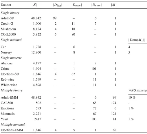
Table 2 Datasets
Dataset |S| |Dbi n| |Dnom| |Dnum| |M|
Single binary
Adult-SD 48,842 99 − 6 1
Credit-G 1,000 2 11 7 1
Mushroom 8,124 4 18 − 1
COIL2000 5,822 5 80 − 1
Single nominal |Dom(M1)|
Car 1,728 − 6 − 1 4 Nursery 12,960 − 8 − 1 5 Single numeric Abalone 4,177 − 1 7 1 Crime 1,994 − 1 101 1 Elections-SD 1,846 4 67 1 1 Red-wine 1,599 − − 11 1 White-wine 4,898 − − 11 1
Multiple binary WKG minsup
Adult-EMM 48,842 − − 6 99 10 % CAL500 502 − − 68 174 -Emotions 593 − − 72 6 1 % Mammals 2,221 − − 67 124 -Yeast 2417 − − 103 14 1 % Multiple nominal Elections-EMM 1,846 4 5 1 62
For each dataset the number of tuples, the number of binary, nominal, and numeric description attributes, and the number of model attributes are given. Further, for the single nominal datasets the number of distinct target values is given, and for the multiple binary case the minsup used for WKG is given
7.1 Datasets
To evaluate the proposed methods, we perform experiments on the datasets listed in Table2. In this table, the datasets are grouped by model/target type. The CAL500,
Emotions and Yeast datasets were taken from the ‘Mulan’ repository4 (Tsoumakas et al 2010). Further, we use the Mammals dataset (Heikinheimo et al 2007), which consists of presence information of European mammals (Mitchell-Jones et al 1999) and climate information.
The two Elections datasets were constructed from data collected by the ‘election engine’ atwww.vaalikone.fibefore the 2011 parliamentary elections in Finland. The data was published by Helsingin Sanomat,5a Finnish newspaper, and it consists of
information about the roughly 2000 candidates that participated in the elections. In
4 http://mulan.sourceforge.net/datasets.html.
the EMM-variant of the dataset, candidate properties such as party, age, and educa-tion are used as descripeduca-tion attributes, while the answers and weights assigned by the candidates to 30 questions are used as model data. For each question, the candidates could choose one from 3 up to 8 answers. In the SD-variant of the dataset, all attributes just mentioned are used as description data, and the number of votes each candidate received in the elections is used as target. In that case, the goal of SD can be inter-preted to be finding candidate properties and answers that result in relatively many votes.
The rest of the datasets are taken from the UCI repository.6 Two variants of the UCI Adult dataset are used: Adult-SD is the commonly used variant, with the binary class label as single target, in Adult-EMM all numeric attributes are considered as description attributes, and all binary attributes as model attributes (except for class, which is not used). For the Crime dataset, the unprocessed ‘unnormalized’ version was taken and pre-processed as follows. First, all non-predictive attributes and potential goals except for violentPerPop were removed. Next, all tuples that have a missing value for violentPerPop were removed. Finally, all attributes with missing values were removed.
7.2 A characteristic multiple model attribute experiment in detail
To study the effects of the proposed search strategies and dominance-based prun-ing in detail, we focus on a sprun-ingle dataset. As we previously presented a detailed SD example invan Leeuwen and Knobbe(2011), we here present an example with multiple model attributes. For ease of presentation, we choose the relatively small
Emotions dataset with WKL as quality measure. From Fig.1 we have already seen that redundancy in the subgroup covers is a problem when a standard beam search is used, and we will now investigate how the newly proposed search strategies improve diversity.
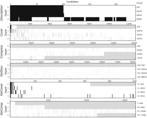
Figure2shows which subgroups are selected for refinement on each level in the beam search performed byDSSD. Clearly, all selection strategies select subgroups from a much wider range than the standard top-100, which is likely to result in more diverse beams. Looking at the upper three plots, we observe that a higher degree of redundancy elimination results in more (high-quality but similar) candidates being skipped; this fully meets our expectations.
Our hypothesis is that the diverse beam selection methods result in more diverse (and therefore less redundant) subgroup sets. To assess this, consider the subgroup covers depicted in Fig.3. Compared to the Beam results shown in Fig.1, it is clear that mining more subgroups and adding a post-processing phase helps to improve diversity (see Beam+PP). Actually, both a visual inspection and the values for CR and H reveal that the results obtained this way are quite similar to those obtained with
Description. The latter is faster though (117s vs 238s) and finds a top-1 subgroup with
higher quality (W K L=0.60 vs W K L=0.56).
Fig. 2 DifferentDSSD subgroup selection strategies in action, on dataset Emotions with WKL as quality
measure. For each level in the beam search, it is shown which candidate subgroups are selected for inclu-sion in the beam (black) and which are ignored (white). Candidates are ordered descending on quality. On the right, the total number of candidate subgroups for each level is shown (candidates not shown are not selected). In the upper three plots,w=100 subgroups are selected on each level, while the number of selected subgroups is shown on the right for the lower three plots
Both Cover and Compress further improve subgroup cover diversity, but do so in different ways. Cover discovers subgroup sets consisting of quite large subgroups (containing 202.1 tuples on average), while Compress finds much smaller subgroups (78.5 tuples on average). The cover-based approach is much more diverse in terms of CR, but the joint entropy of the results of the compression-based method is also quite high.
Then there are the sequential and weighted covering approaches. Sequential cov-ering finds only 19 subgroups, after which the resulting dataset consists of too few tuples to continue (|S|<=mi nCov). The Weighted approach finds results that seem quite similar—and are possible even more diverse—than those obtained with Cover. The subgroups are of similar size (211.5 tuples on average), the best subgroup found is of almost the same quality (but slightly lower), and both CR and H indicate slightly more diverse subgroup covers. There is one important difference however, as Cover needed only 4 min to run, while the weighted covering approach needed 112 min. While achieving similar results, the cover-based strategy provides a significant 28× speed-up with respect to weighted covering!
Fig. 3 Subgroup covers obtained with six search strategies. Shown are the covers (in black) of the
sub-groups obtained on Emotions with WKL. CR and joint entropies (H) calculated on the subgroup sets are shown on the right
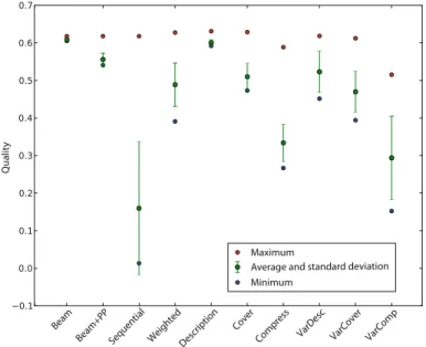
In Sect. 4 we stated that it is our goal to find non-redundant sets of high-qual-ity subgroups. It is therefore important that the maximum qualhigh-qual-ity of a subgroup set, the highest quality obtained by any subgroup, is as high as possible. To assess this, consider the qualities of the obtained subgroup sets depicted in Fig.4. All alterna-tive approaches clearly give more diverse results than Beam, as we already saw from the subgroup covers; the lower average qualities and larger standard deviations are natural consequences of the diversity enforced by subgroup set selection. Weighted,
Description and Cover attain higher maximum qualities than the rest, confirming that
diversity may contribute to find higher quality subgroups. Sequential covering and the compression-based approaches do not seem to be good alternatives when high quality is a primary requirement.
Finally, let us consider an example of the effect of dominance-pruning. After the first phase ofDSSD, the beam search, the descriptions of the 10,000 discovered sub-groups consist of 43,258 conditions in total. After applying the pruning phase, this has
Fig. 4 Qualities of subgroup sets obtained with different search strategies
been reduced to 34,706 conditions, meaning that 8,552 conditions could be removed! Meanwhile, average quality has increased from 0.509 to 0.522. This clearly demon-strates the usefulness of dominance-based pruning of individual subgroups; subgroup descriptions become shorter and thus simpler, while quality increases.
7.3 Quantitative results
We now present results obtained on a large number of experiments performed on all datasets, to show when it may be beneficial to use theDSSD algorithm, and when it is better to use existing methods. Primary objectives are to discover subgroup sets that are (1) high quality and (2) diverse in (3) as little computation time as possible. Results are aggregated per target type, with the multiple binary and nominal model attribute types combined.
Regarding the first two objectives, a search strategy is better than others if it more often achieves (1) a higher maximum quality, (2) a lower CR, and (3) a higher joint entropy. We quantify this using average rank results. For each combination of data-set, quality measure and search strategy, an experiment was conducted and ranked with respect to (1) maximum quality (ϕmax, descending), (2) CR (ascending), and (3) joint entropy (H, descending), stratified by search strategy. Tied ranks are assigned the average of the ranks for the range they cover. Finally, all ranks for a specific search strategy are averaged.
Results obtained for the single binary setting are shown in Table3. Of all search strategies, Beam, DFS and DFS+PP result in most redundancy, and the depth-first search strategies also reach less high quality (due to the fixed order in which attributes
Table 3 The single binary case, aggregated over Adult-SD, Credit-G, Mushroom, and COIL2000 with WRAcc and WKL
Search strategy Exp avg Subgroup set avg Rank avg
t (min) |R| Descr. Size CR H ϕmax CR H
DSSD-Desc 21.1 94 4.6 4328 1.18 2.36 4.3 5.7 5.0 DSSD-VarDesc 18.8 25 4.3 1161 1.07 3.47 5.4 5.2 4.8 DSSD-Cover 59.8 100 4.3 5642 0.63 5.01 4.3 2.7 2.9 DSSD-VarCover 1.8 26 3.3 758 11.04 3.37 4.8 7.1 4.6 Beam 11.4 100 4.8 4280 1.33 1.17 4.7 7.6 8.3 Beam+PP 12.7 100 4.0 4986 1.03 2.43 4.7 5.0 5.8 Beam-Seq 72.2 27 3.7 3224 0.35 6.28 4.7 2.0 3.4 Beam-Weighted 427.9 100 4.8 6290 0.35 7.58 4.3 1.9 1.6 DFS 551.0 100 4.9 2067 1.16 1.55 7.4 8.0 8.8 DFS+PP 577.8 100 3.3 2099 1.03 2.44 7.4 7.0 8.0
The following averages over all experiments are shown: the time (in minutes) and the average number of discovered subgroups, the number of conditions per subgroup description (descr.), subgroup sizes, CR and joint entropy H. Description and subgroup sizes are first averaged per subgroup set resulting from an experiment, and then averaged over all experiments. On the right, average ranks are given as obtained by ranking experiments stratified by search strategy, for maximum quality, CR and joint entropy
are refined). Beam-Seq, VarDesc and VarCover result in a similar number of subgroups;
Beam-Seq gives larger subgroups that have more diverse covers, but the variable-size
approaches are much faster.
Cover and Weighted achieve high-quality and quite diverse subgroup sets (in terms
of CR and H), but the former is roughly seven times faster on average. The fixed-size description-based approach seems a reasonable alternative if one wants results quickly, as it attains high quality results in little time.
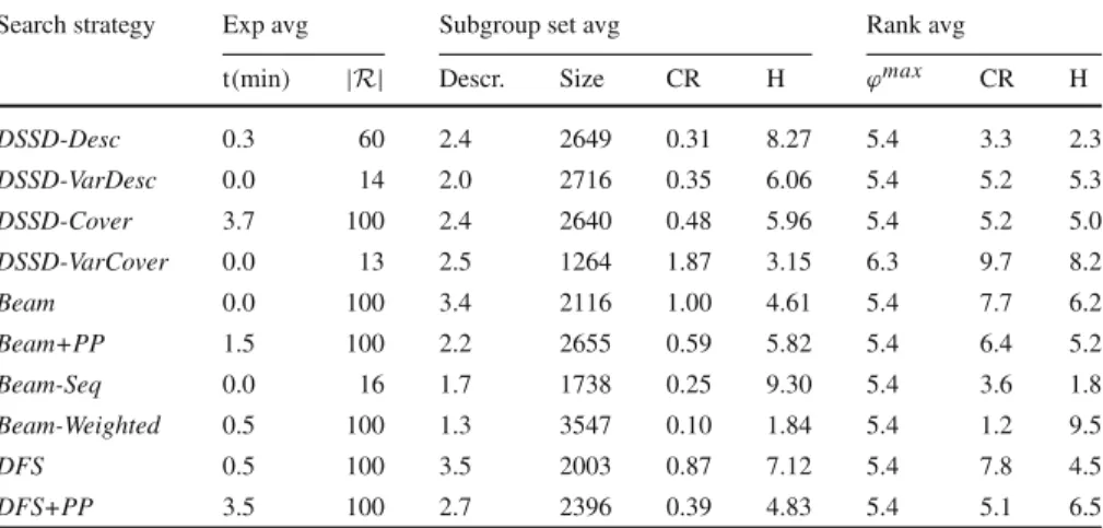
Table4shows that runtimes, subgroup sizes and maximum qualities are quite com-parable among the search strategies in the single nominal setting. Desc seems to perform very well in terms of cover diversity, while CR and joint entropy for
Beam-Weighted are rather inconclusive.
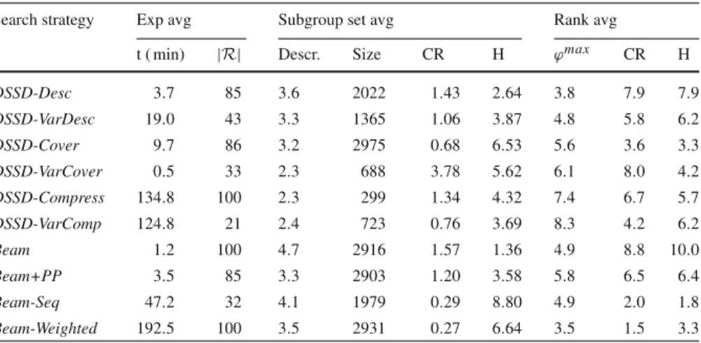
The results of the single numeric case, presented in Table5, are more interesting, as the differences are larger. Weighted covering seems to do a very good job: the maximum qualities rank quite high and both the average ranks for CR and H are out-standing. However, the runtime is problematic when compared to Cover, exhibiting a staggering difference of a factor 23. CR and joint entropy obtained with cover-based selection indicate a bit less diversity, but the difference does not seem too large and
Cover does rank higher with respect to maximum quality. Also, it is important to
observe that Cover does better than Beam+PP, except that it is slower.
We previously observed that sequential covering gives few yet very diverse sub-groups of reasonable quality. However, it isn’t particularly fast and we know from its definition that it discourages overlapping subgroups. This makes the discovery of many possibly interesting subgroups highly unlikely and we therefore discard sequen-tial covering as a serious competitor. The VarDesc and VarCover approaches also return