Models and algorithms for dominance-constrained stochastic programs with recourse

(1)

Models and Algorithms for

Dominance-Constrained Stochastic

Programs with Recourse

Von der Fakult¨

at f¨

ur Mathematik der

Universit¨

at Duisburg-Essen

zur Erlangung des akademischen Grades eines

Dr. rer. nat.

angenommene Dissertation

von

Herrn Dipl.-Math. Dimitri Drapkin

Referent: Prof. Dr. R¨

udiger Schultz

Koreferent: Prof. Dr. Maarten H. van der Vlerk

(2)

(3)

Acknowledgements

It gives me great pleasure to thank first and foremost my supervisor Pro-fessor Dr. R¨udiger Schultz for his constant support throughout my time as his student - without his support this thesis would not have been possible. I have been extremely lucky to have a supervisor who cared so much about the advancements of my work above and beyond pure mathematical questions.

I owe my deepest gratitude to Dr. Ralf Gollmer for introducing me to the world of C, Linux, CPLEX, etc., and providing invaluable advice in many desperate situations.

Completing this work would have been all the more difficult were it not for the support and friendship provided by the other members of the working group “Optimization and Algorithmic Discrete Mathematics”.

A very special word of thanks goes to the former members of this group Dr. Uwe Gotzes and Oliver Klaar for their contributions to the foundations of this thesis.

Finally, I must express my gratitude to my wife, Svetlana, for her continued support and encouragement during all the ups and downs of my research.

(4)

Abstract

We consider optimization problems with stochastic order constraints of first and second order posed on random variables coming from two-stage stochastic programs with recourse. We clarify the theoretical relevance of these specific problems, and contribute to improving their computational tractability. For the latter, we review and enhance mixed-integer linear programming (MILP) equivalents. These exist for either mixed-integer or continuous variables in the second stage. Algorithmically, our focus is on developing tailored cutting-plane decomposition methods for these models.

Stochastic mixed-integer programming, stochastic dominance, decomposi-tion methods, cutting-plane methods, risk aversion.

(5)

Zusammenfassung

In der vorliegenden Dissertationsschrift befassen wir uns mit stochastischen Optimierungsproblemen unter Nebenbedingungen, die mithilfe stochastischer Ordnungen formuliert sind. Hierbei konzentrieren wir uns auf stochastische Dominanz erster Ordnung und die steigende konvexe Ordnung, wobei beide Ordnungen in unserem Fall auf Zufallsgr¨oßen operieren, welche Optimalwerten zweistufiger stochastischer Optimierungsprobleme mit Kompensation entspre-chen.

Wir stellen die theoretische Relevanz der vorliegenden Problemklasse heraus und tragen zur Entwicklung von effizienten Lösungsverfahren bei. Um Letzteres zu erreichen untersuchen und erweitern wir bestehende gemischt-ganzzahlige lineare Repräsentationen dieser Probleme und entwickeln maßgeschneiderte Dekompositionsverfahren. Der Schwerpunkt dieser Arbeit liegt dabei auf der Entwicklung und Implementierung besonders effizienter Lösungsansätze für den Fall mit linearer Kompensation.

Stochastische gemischt-ganzzahlige Optimierung, Stochastische Dominanz, Dekompositionsverfahren, Schnittebenenverfahren, Risikoaversion.

(6)

(7)

List of Figures

3.1 Overview of SP Models . . . 26 3.2 Information Constraints . . . 28

List of Tables

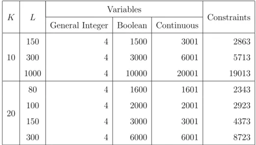
7.1 Dimensions of mixed-integer linear programming equivalents (investment planning) . . . 85 7.2 CPU times in seconds for investment planning instances . . . . 86 7.3 Dimensions of mixed-integer linear programming equivalents

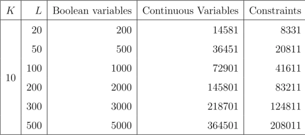
(Sudoku puzzling) . . . 88 7.4 CPU times in seconds for Sudoku instances . . . 89 7.5 Dimensions of mixed-integer linear programming equivalents

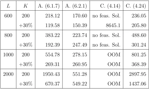
(Energy Retailer Problems) . . . 90 7.6 CPU times in seconds for Energy Retailer Problems . . . 90

(10)

(11)

List of Abbreviations

cdf cumulative distribution function. 10 CPT cumulative prospect theory. 6 DARA declining absolute risk aversion. 5 EUT expected utility theory. 5

FSD first-order stochastic dominance. 8 ICC integrated chance constraints. 27 ICV increasing concave order. 12 ICX increasing convex order. 18

MILP mixed-integer linear programming. 2 PSD prospect stochastic dominance. 9

RDEUT rank-dependent expected utility theory. 6 rv random variable. 10

SD stochastic dominance. 7 SP stochastic programming. 1

(12)

Symbol Index

X,Y real-valued random variables

FX, FY cumulative distribution functions ofX resp. Y

¯

FX survival function of X 11

F_X−1 inverse distribution or first quantile function ofX 16

F_X(2) second performance function of X 12

F_X(−2) second quantile function of X 17

(n) nth order stochastic dominance relation 7

IE,R,IE,ρ mean-risk dominance relation for gains resp. losses 13,30

icx increasing convex ordering relation 18

R, ρ risk functionals on gains resp. losses 13,30

A acceptability functional 15

IE[t−X]+ expected shortfall below targett, cf. Remark 2.2.8 14

IE[X−t]+ expected excess above target t 19

V@Rα value-at-risk at level α 16

T V@Rα tail value-at-risk at level α 16

CV@Rα conditional value-at-risk at level α 20

QIE expected recourse function 29

Φ second-stage value function 28,44

f(x, ω) rv reflecting overall costs for a first-stage decision x 30,44

2Ω power set of Ω 63

(13)

Chapter 1 Introduction

Good decisions have always been connected with mastering some kind of un-certainty. In former times experience and common sense used to be the only aids to find a good path. Starting from the middle of the twentieth cen-tury, stochastic programming (SP) emerged, at the interface of probability and optimization theory, to become a discipline of science aiming at explo-ration, development and improvement of models for decision making under uncertainty.

Today, stochastic programming has a great variety of applications from sports, e.g., yacht racing [Phi05], over management of risks related to natural disasters, e.g., of flood and seismic risks [EE05], to manifold applications in finance [DHv02]. Even the problem of finding an optimal shape for an elastic body (e.g., a cantilever) under uncertain loading configurations was recently formulated and solved by means of (infinite-dimensional) stochastic program-ming, see [CHP+09].

Though the achievements in this field have been remarkable, a sensible han-dling of uncertainty and risks seems to be more important than ever to master the challenges of the day. Various aspects of risk management are subject to constant debate in science and society. Also the mathematical models are con-stantly getting larger and gain complexity, providing a motivation for ongoing

(14)

Chapter 1. Introduction

research.

In the present thesis, we will deal with a specific decision making framework of dominance-constrained stochastic programs with recourse. Our aim will be, on the one hand, to clarify the theoretical relevance of this problem class in view of recent developments in the adjacent fields of decision theory, risk modeling and stochastic programming. On the other hand, to strengthen the relevance of dominance-constrained problems in practical decision making under uncertainty, we will concentrate on the algorithmic aspects of these problems proposing new and enhancing existing solution techniques.

The thesis is structured as follows. In Chapter 2, we define relations of stochastic dominance and review their decision theoretical background. Also some computationally tractable representations for SD and an outline of its connections with the related concept of risk measures are presented. In Chap-ter 3, we expose how to incorporate SD into the established optimization framework of SP, and introduce our problem class of dominance-constrained stochastic problems with recourse. In Chapter 4, mixed integer linear pro-gramming (MILP) equivalent formulations for such problems are developed and enhanced. Starting from Chapter 5, we concentrate on the case of lin-ear recourse, i.e., on problems without integer variables in the second stage. Model equivalents based on duality are derived for these problems in Chap-ter 5, whereas cutting plane decomposition methods are proposed in ChapChap-ter 6. Lastly, computational results presented in Chapter 7 indicate the effectiveness of our approach and conclude the thesis.

(15)

Chapter 2 Comparing Risks for Decision

Making under Uncertainty

2.1 Stochastic Dominance and Decision

The-ory

Decisions we are making today tend to have prospects observable in the future, only. The problem of making good decisions prior to having the exact infor-mation from the future, is the fundamental matter of stochastic programming. Thus, stochastic programming can be understood as optimization under in-formation or nonanticipativity constraints. Though we cannot anticipate the future, in the present thesis we assume, that all relevant uncertain quantities can be identified and modeled as random variables with distributions known to the decision maker.1

Once the basic model is set, the question of a sensible comparison of random outcomes arises, since it has to be clarified what a ”good” decision should be. The first sound idea of such a comparison yielded the concept of the expected

1_{The problem of selecting an appropriate basic probability model is referred to as the}

am-biguity problem, cf. [RP07] and the discussion therein, in contrast to the so-calleduncertainty problem treated here.

(16)

Chapter 2. Comparing Risks for Decision Making under Uncertainty

value, introduced in the 17th century by Blaise Pascal as a ”fair” solution for the ”Problem of Points”2_{. Symptomatically, the question of what should be}

considered ”good” or ”fair” was even then not only a mathematical question. In today’s terms, and at least in case of many repetitions of the same setting, optimizing the expected value of the prospects is justified by the Law of Large Numbers. In fact, the average of a prospect will converge with the number of repetitions to its expected value, meaning that the obtained solution would be optimal on average.

The drawback of the expectation based approach is its complete neglect of the risk incurred by concrete realizations of the random outcome. Ignoring the risk, however, may easily lead to inferior or even completely implausible decisions. One famous example of such a situation is that of the St. Petersburg Lottery: a game with infinite expected payoff, for which there is ”no person of good sense, who would wish to give 20 coins”3.

To resolve this difficulty, Daniel Bernoulli proposed to measure the utility of an outcome numerically (as the logarithm of one’s monetary possessions) and to optimize the ”mean utility” instead of the expectation itself.4 _{Bernoulli’s}

work inspired the concept ofmarginal utility and gave rise to acardinal utility theory, which made the notion of utility indispensable in economics.

However, it proved problematic (if not impossible) to determine utility func-tions explicitly.5 _{This difficulty led to the development of normative models,}

starting from the beginning of the 20th century. In these models, systems of a

2_{According to [Kat98, Chapter 11.3], the discussion of this problem belongs to the earliest} beginnings of probability theory.

3_{As Gabriel Cramer put it in his correspondence with Nicolas Bernoulli in 1728, cf. [Ber75]} for the edifying discussion of St. Petersburg paradox.

4_{Cf. [Ber54] for the English translation of D. Bernoulli’s seminal ”Exposition of a New} Theory on the Measurement of Risk”, originally published in 1738 in Latin.

5_{The effort in utility measurement was considerable and produced some interesting} con-cepts (e.g., Edgeworth’s hedonimeter), cf. [Col07]. In the modern economic discourse this

experienced utility was largely replaced by decision utility which refers to the prospect’s weight in decisions and can be inferred from observed choice, cf. [KWS97].

(17)

2.1. Stochastic Dominance and Decision Theory

few axioms were proposed to describe preferences which should be consistent across different choice problems.

A (preliminary) culmination of these efforts was the development of the expected utility theory (EUT) by von Neumann and Morgenstern. In their fundamental work [VNM44], a notion of arational decision maker - defined as an agent obedient towards a given set of four intuitive axioms - was introduced. This rational decision maker was proven to possess a utility functionu(·)6 _such

that he would prefer a prospectY to Xiff

IE[u(Y)]≥IE[u(X)].7 _(2.1)

In the framework of EUT the study of attitudes towards risk is of special importance. A decision maker is called risk-averse if he prefers the expected value of a prospect to the random prospect itself, i.e., his utility function is concave with

IE(u(X))≤u(IE(X)). (2.2)

Otherwise, he is called risk-seeking with a convex utility.8 _{To compare risk}

aversion between individuals9 some measures of risk aversion were introduced, most notably theArrow-Pratt measure of absolute risk-aversion ρ(x) :=−u_u000₍(_xx₎),

cf. [Pra64, Arr65]. With the help of this measure it is possible to formulate the plausible assumption of declining absolute risk aversion (DARA) which is characterized by a non-increasing ρ (ρ0 ≤0), cf. [Vic75].10

Being a powerful tool for decision making under uncertainty, EUT recently came under pressure, both from the descriptive and the normative side. On

6_{Such utility functions can be determined up to an affine transformation through the} analysis of a decision maker’s preferences betweensimple lotteries. For a more practically successful approach the author refers to [ADH77].

7_{From now on we assume the utility functions to be differentiable sufficiently often, all} expected values are assumed to exist.

8_{Both observations are a direct consequence of Jensen’s inequality.}

9_{This task is not straightforward because utility functions are lacking uniqueness.} 10_{E.g., Bernoulli’s logarithmic utility function exposed DARA.}

(18)

the one hand, there is empirical evidence of behavioral patterns which system-atically violate EUT, cf. [All53, KT79].11 _{For example, individuals}

systemat-ically overweight low-probability events and show different attitudes towards gains and losses with respect to the status quo (e.g., buy lottery tickets and insurance contracts simultaneously). On the other hand, fundamentally dis-tinct notions of attitude towards risk and attitude towards wealth coincide in EUT thus leading to the question whether these concepts could be decoupled. Several generalizations of EUT have recently been proposed to resolve these drawbacks.

Therank-dependent expected utility theory (RDEUT) elaborated on the ob-served subjective probability distortion. It was originally presented by Quiggin ([Qui82]) and developed for a special case by Yaari ([Yaa87])12_{under the name}

dual utility theory. From a (weaker) set of axioms a utility function u(·) and a nondecreasing probability transformation function q(·) : [0,1]→ [0,1] were proven to exist, s.t. a prospectY is preferred to Xiff

Z

u(t)d(q◦FY)(t)≥

Z

u(t)d(q◦FX)(t). (2.3)

A further generalization of EUT is the highly praised cumulative prospect theory(CPT) of Kahneman and Tversky, cf. [KT92].13 In this theory, gains and losses are considered separately: the utility function is assumed to be convex for the losses and concave for the gains (i.e.,u(·) is S-shaped); separate reverse S-shaped probability distortion functions are proposed for either case. While most experimental studies support CPT (thus explaining its popularity), we refer to [LL02a, LL02b] and the references therein for some critical findings.14

So far, we have compared the riskiness of a prospect from the individual

11_{The work [KT79] is regarded as the fundamental paper in} _{behavioral economics}_. 12_{In Yaari’s version,}_u₍_·_{) is assumed to be the identity function and the probability} trans-formation function is referred to as adual utility function.

13_{In particular for the development of CPT, Kahneman received the Nobel Prize in} Eco-nomics in 2002.

14_{In the quoted articles particularly the S-shape of a utility function is rejected by studies} envolving mixed (partly positive, partly negative) prospects. However, [Wak03] shows, that

(19)

perspective of a given decision maker, pointing out the properties of his utility functions connected with his attitude towards risk. In practice, the knowledge of the concrete shape of a utility function is at best partial and it makes sense to consider classes of utility functions characterizing typical risk attitudes.

This idea leads us to a more general approach ofstochastic dominance (SD), which will be the main subject of the present thesis. In the context of decision theory, SD enables a direct comparison of prospects by means of EUT. More precisely, one prospect will be said to dominate the other if it is preferred by all individuals with utility functions in a given class.

Under the assumed preference of more money to less, the most general class

U1 of utility functions will include all nondecreasing functionsu(with u0 ≥0).

We have already seen that in EUT risk-aversion is equivalent to concavity of the utility function, hence the classU2 will contain all concave utility functions

from U1 (u0 ≥0, u00 ≤0).

More generally, one could consider utility functions whose derivatives alter-nate in sign, i.e, belong to the class Un:={u∈ Un−1 : (−1)nu(n) ≤0}, n > 1,

whereby the economic interpretation for n > 3 is not evident.15 _The

impor-tance of U3 is related to the fact that U3 ⊃ UDARA :={u∈ U2 :u0 6= 0, ρ0 ≤0}

and the conditions in U3 are easier to check.16

Corresponding stochastic dominance relations are then defined in a straight-forward way:

Definition 2.1.1. For random variables X andY, we define Y to dominate X w.r.t. nth order stochastic dominance, written X(n)Y iff

IEu(X)≤IEu(Y)∀u∈ Un. (2.4)

due to probability distortion, the studies actually support the CPT - an argument countered in [LL03] for some special cases.

15_{Such classes of utility functions were generalized for all real numbers}_{n >}_{0, cf. [Fis76,} Fis80].

(20)

Stochastic dominance w.r.t. DARA utility functions is defined analogously.17 Remark 2.1.2. In the present thesis, we define all dominance relations in the so-called weak form, i.e., we do not exclude the possibility of simultaneously XY and YX. For any (weak) dominance relation ””, the corresponding strict form ”≺” is given through the standard rule

X≺Y⇔XY and Y6X. (2.5)

In the generalizations of EUT the defined dominance rules only make sense if they are consistent with the underlying decision model. More precisely, ifY is preferred toXw.r.t. a dominance relation, it should also be preferred in the corresponding model by all decision makers with utility functions in the given class.18

In the rank-dependent expected utility theory (RDEUT), consistency fol-lows for first-order stochastic dominance (FSD) from monotonicity of the prob-ability weighting function q in view of (2.3), cf. [Qui82, Proposition 3]. Due to its interpretation (as a general preference of more to less), consistency with FSD is such a fundamental property, that it holds for most generalizations of EUT.19 FSD is also sometimes referred to as the axiom of ”absolute prefer-ence”, because it can be used to axiomatize RDEUT ([Qui92, Yaa87]).

Lacking consistency with FSD of the original version of the prospect theory ([KT79]), was considered such a large drawback that it partly inspired the development of CPT ([KT92]) to elaborate on this issue.

The situation with second-order stochastic dominance (SSD) in the gener-alized models is more complex. In RDEUT a decision maker is risk-averse (in the sense of preferring certainty over risk, see above) iff he is characterized

17_{For more details on this dominance relation the author refers to [Vic75, Vic77].} 18_{For EUT this consistency requirement is immediate from the definition of dominance} relations.

19_{Especially those generalizations of EUT concerning relaxation of the independence} ax-iom and partly even the transitivity axax-iom, cf. [Lev92, p. 559 - 560].

(21)

by a concave utility function and a pessimistic transformation of probabili-ties.20 _{SSD consistency is preserved if both}_u₍_·_{) and}_q₍_·_{) are concave, which is}

a weaker condition than risk-aversion, cf. [Qui92, p. 80].

Due to the proposed S-shape of utility functions, which explicitly assumes a partly risk-seeking behavior of the decision maker, CPT is of course not consistent with SSD. The notion ofprospect stochastic dominance(PSD) which considers all S-shaped utility functions and is consistent with prospect theory was proposed in [LW98, Lev06]. However, consistency problems with CPT arise in view of reverse S-shaped probability distortion functions proposed there, cf. [LL02a, p. 1065]. Recently, several even more general classes of dominance relations have been proposed which also take account of the relevant probability distortion functions, cf. [BH06]. Nevertheless, the author takes the view that a broadly accepted and computationally tractable stochastic dominance theory for the CPT still has to be developed.

In view of the above discussion, in the present thesis we will consider the FSD relation, because it is the most fundamental SD rule consistent with all most prominent decision models, and the SSD relation because of its account for risk-aversion in EUT and its good mathematical and computational prop-erties, cf. [DR03].

In the context of decision theory, SD was introduced by a number of au-thors starting from 1960’s, most notably Quirk and Saposnik ([QS62]), Fish-burn ([Fis64]), Hadar and Russell ([HR69]), Hanoch and Levy ([HL69]) and Rothschild and Stiglitz ([RS69]).21 A detailed survey of SD rules mainly from the economical perspective can be found, e.g, in [WF78] and [Lev92].

20_{Pessimism means that bad outcomes receive larger and good outcomes smaller} proba-bilities. For the exact definition and the proof see [Qui92, pp. 77].

(22)

2.2 Stochastic Orders and Measures of Risk

The concept of SD is the decision-theoretical counterpart of the more general concept of stochastic orders, which was developed in statistics starting from the late 1940’s, cf. [MW47], [Bla51, Bla53] and [Leh55] for early references22 and [MS02], [SS07] for a contemporary discussion.

Stochastic ordering aims at imposing sensible orders23 _{on the set of}

cumu-lative distribution functions (cdf) of real-valued random variables (rv) defined on a probability space (Ω,F, IP). In the present thesis, ordering of rvs will not be distinguished from ordering of their corresponding cdfs. In these terms, we have seen in the previous section that EUT imposes a total ordering (through (2.1)) in case the utility function is given, and a partial ordering through SD rules. Another possibility to obtain ordering relations will employ acceptabil-ity and risk functionals defined on rvs24, which we will discuss in the present section focusing on their relations to SD.

As we have pointed out above, SD relations were developed for decision makers preferring big outcomes to small, so that a large body of literature exists for this case. On the other hand, some important risk functionals have more natural interpretations for rvs representing losses instead of gains. Starting from the classical setting, we will illustrate here the transition from the one case to the other. In this way, we will obtain the intuition and the representations we will need in the main part of the thesis for the discussion of our minimization framework.

22_{These works were in turn inspired by earlier findings in majorization theory, cf. [HLP34]} and [MOA11] for an overview.

23_{Formally, a (partial) order is a reflexive, transitive and antisymmetric binary relation} over an arbitrary set. The order is called total if any two elements in the set are comparable under the relation.

24_{More precisely, we will use only}_{law-invariant} _or_{version-independent} _{functionals, which} depend on the cdf only, cf. [RP07, Definition 2.1].

(23)

2.2. Stochastic Orders and Measures of Risk

2.2.1 Preference of Large Outcomes

In the context of statistics, SD rules are equivalently expressed through a pointwise comparison of some performance functions constructed from a rv’s cdf. For FSD, this performance function is the cdf itself and the following (primal) characterizations hold.

Proposition 2.2.1. For rvs X,Y∈(Ω,F, IP)with cdfs FX and FY the

follow-ing statements are equivalent:

(i) X(1)Y;

(ii) FX(t)≥FY(t) ∀ t∈R;

(iii) there exists a probability space ( ˆΩ,Fˆ,IPˆ) and random variables Xˆ and Yˆ with marginals FX and FY such that X(ˆˆ ω)≤Y(ˆˆ ω) for all ωˆ ∈Ω;ˆ

(iv) IP(X> t)≤IP(Y> t) ∀ t∈_R.

Proof. (i)⇔(ii) Theorem 1.2.8 in [MS02], (ii)⇔(iii) Theorem 1.2.4 in [MS02], (iv)⇔(ii) clear.

In other words, the preference of more to less in EUT can be equivalently described by a pointwise comparison of cdfs (which implies that the smaller rv should take smaller values with a higher probability) and is closely related to the simple pointwise comparison of rvs. Thus, being the most fundamental version-independent ordering concept for rvs, FSD is often just referred to as the (usual) stochastic order, cf. [SS07, p. 3].

The function ¯FX(t) := IP(X > t) from the representation (iv), which we will use to derive computationally tractable representations for FSD starting from Chapter 4, denotes the so-called survival function, well-known, e.g., in actuarial sciences, cf. [Pro11, p. 194].

(24)

For SSD, computationally more tractable representations can be derived by means of the second performance function

F_X(2)(t) := t Z −∞ FX(α)dα ∀ t∈R (2.6) as follows.

Proposition 2.2.2. For rvs X,Y ∈ L1(Ω,F, IP) with cdfs FX and FY the

following statements are equivalent:

(i) X(2) Y;

(ii) IE[t−X]+ ≥ IE[t−Y]+ for all t ∈ R, where [α]+ := max(α,0) is the

positive part of α;

(iii) F_X(2)(t)≥F_Y(2)(t) for all t ∈_R. Proof. See Theorem 4.A.2 in [SS07].

Due to the definition of SSD by nondecreasing concave utility functions in Definition 2.1.1 this order is also often called the increasing concave order (ICV). The observation that only a small subset of these functions is sufficient to fully characterize ICV leads to (ii). From the integral condition (iii) it is here again immediate that FSD implies SSD, because (iii) can be interpreted as a requirement for the area enclosed between the two cdfs to be non-negative up to every point t, which is a weaker condition than a pointwise comparison of the cdfs.

Though the above representations are more tractable, checking both domi-nance relations implies comparison of performance functions on infinitely many points, which is a complex task. In fact, a much easier approach to compare distributions was developed in probability theory from its very beginnings: namely the study and comparison of cdfs by their relevant parameters. These parameters are distinguished between a value dimension and a risk dimension.

(25)

Since Pascal, the value dimension is typically represented by the expected value of the prospect. At this, it follows directly from the definitions that

X(i) Y=⇒IE(X)≤IE(Y), for i= 1,2, (2.7)

because the identity function is both increasing and concave.

To address the risk dimension, a wide variety of (version-independent) risk functionals R(·) on the space of rvs has been defined which characterize the riskiness of the whole cdf by a scalar. Keeping both dimensions separate leads to a bi-criteria decision problem, while the relative importance of value to risk represents therisk aversion in this context.25 _{These considerations lead to the}

definition of the following relations.

Definition 2.2.3. For rvs X,Y∈ L1(Ω,F, IP), we define

XIE,RY iff IE(X)≤IE(Y) and R(X)≥ R(Y); (2.8) and

XIE−λR Y iff IE(X)−λR(X)≤IE(Y)−λR(Y), (2.9) where λ >0 is an assumed degree of risk aversion.

The relation (2.8) is called mean-risk dominance, whereas the approach of maximizing IE(X)−λR(X) constitutes the so-called mean-risk approach. This approach was pioneered by Markowitz in his seminal work [Mar52] and still is very popular among practitioners and researchers due to its excellent computational tractability.

However, to justify the mean-risk approach theoretically, compatibility with the findings of decision theory has to be verified. In particular, the risk func-tional should be such that the model becomesconsistent with FSD and prefer-ably also with SSD (to account for risk-aversion in EUT) in the sense of the following definitions.

(26)

Definition 2.2.4. The mean-risk model (IE,R) is said to be consistent with i-th order SD if

X(i)Y=⇒XIE,R Y, (2.10)

and λ−consistent with i-th order SD if

X(i) Y=⇒XIE−λR Y (2.11) for someλ >0 and i= 1,2.

Thus, a strict maximum of a λ−consistent model will not be dominated w.r.t. the corresponding dominance relation, cf. Section 3.1.3. Clearly, (2.10) implies (2.11) for allλ >0 and consistency with SSD implies consistency with FSD (but not vice versa).

The seminal mean-risk model presented in [Mar52] considered the variance as a risk functional. This model was heavily criticized for being inconsistent with FSD. Also variance as a risk measure is in many ways not adequate.26

On the other hand, e.g., the expected shortfall27 below some fixed target t

defined asIE[t−X]+ is a sensible risk measure, which yields an SSD-consistent

mean-risk model in view of Proposition 2.2.2 (ii). Moreover, in this way SSD can be described as a continuum of constraints on this risk measure.28

Examples of sensible risk functionals taking into account all gainsbelow the mean, which are not consistent but only 1-consistent with SSD (cf. [OR99, OR02]) are lower absolute semideviation

ASD−(X) :=IE([IE(X)−X]+) = 1 2 Z ∞ −∞ |t−IE(X)|dIPX(t) (2.12)

26_{Despite its many drawbacks, the mean-variance model attracted much attention and} led, e.g., to the development of the highly praised Capital Asset Pricing Model of portfo-lio optimization, cf. [Sha64]. For special classes of distributions (most commonly normal distributed rvs are assumed) the model is also even consistent with SSD, cf. [Big93].

27_{The term} _{expected shortfall} _{is also frequently used in a different meaning, cf.} Re-mark 2.2.8.

28_{These constraints are closely related to} _{integrated chance constraints} _{(3.5), also cf.} [KH86].

(27)

and lower standard semideviation

ST D−(X) := q IE([IE(X)−X]2 +) = s Z IE(X) −∞ (IE(X)−t)2_dIP X(t). (2.13)

To elaborate on the desirable properties for risk functionals, axiomatic def-initions were proposed in [ADEH99], where the notion of coherence was intro-duced. A coherent risk functional then complies with the following axioms: (R1) Antimonotonicity: X≤Y a.s. implies that R(X)≥ R(Y);

(R2) Convexity: R(tX+ (1−t)Y)≤tR(X) + (1−t)R(Y)∀t∈[0,1]; (R3) Translation antivariance: R(X+a) = R(X)−a∀a∈_R;

(R4) Positive homogenity: R(tX) =tR(X)∀t≥0.

A mirror image to risk functionals are acceptability functionals or safety measures, which assess the acceptability of the cdf instead of its riskiness. These functionals should comply with monotonicity (A1), concavity (A2) and translation equivariance (A3) axioms, which are the counterparts to (R1)-(R3), cf. [RP07].29 Moreover, if A is a positively homogeneous acceptability functional then R(X) :=−A(X) will be a coherent risk functional. Of course, higher acceptability will imply higher preference of a decision maker.

In view of Proposition 2.2.1 (iii), the monotonicity axiom for acceptability functionals is equivalent to the following requirement of isotonicity with FSD

X(1)Y=⇒ A(X)≤ A(Y), (2.14)

which once again underlines the importance of the order. Analogously, con-sistency of the corresponding mean-risk models with FSD has an axiomatic meaning for coherent risk functionals.

Two of the most important acceptability functionals have close relations to the so-called dual representations of the stochastic orders proposed in [OR02], which are characterized with the help of quantiles.30

29_{The axioms for acceptability functionals can be found in A.3.1.} 30_{For the definition of a quantile we refer to A.1.}

(28)

Let F_X−1 : [0,1] → _R¯ denote the (left-continuous) inverse distribution or first quantile function of a distribution function FX, defined as

F_X−1(p) := inf{t:FX(t)≥p} for 0< p≤1. (2.15)

The infimum is attained for 0< p <1 since cdfs are continuous from the right, and we can define the first acceptability functional as follows.

Definition 2.2.5. The left α-quantile

V@Rα(X) :=F_X−1(α) (2.16) is called value-at-risk at level α.

Though V@Rαis not concave, it is widely used and very relevant in many decision models, cf. [RP07, pp. 57] and the references therein.31 _Directly

from Proposition 2.2.1 (ii) we now get another characterization for FSD as a continuum of constraints on theV@Rα acceptability functional.

Proposition 2.2.6. For random variables X and Y the following statements are equivalent:

(i) X(1) Y;

(ii) V@Rα(X)≤V@Rα(Y) for all α∈]0,1].

The average of the left quantiles below α now gives another important acceptability functional with nice mathematical properties.32

Definition 2.2.7. The tail value-at-risk at level α, written T V@Rα, with 0 < α ≤ 1 is defined as T V@Rα(X) := 1 α α Z 0 F_X−1(t)dt. (2.17)

31_{In the case of rvs representing losses, V@R}

αhas a natural interpretation of a quantile

risk measure, that we will discuss in Section 2.2.2. 32_{In fact,} ₋_{T V}_@_R

(29)

Remark 2.2.8. Definition 2.2.7 is due to [Ace02], where−T V@Rα was called

α-Expected Shortfall. T V@Rα is also referred to as the average value-at-risk in [FS11], which is a major reference in financial mathematics. In the lit-erature, different names are frequently used synonymously, which is, unfortu-nately, a constant source of confusion. To distinguish between the functionals, we will use the term T V@Rα as above (cf. [OR02]) and CV@Rα as in Defi-nition 2.2.14 (cf. [Pfl00]).

Interestingly, the second quantile function

F_X(−2)(p) := p Z

0

F_X−1(t)dt for 0< p ≤1, (2.18) which we used for the definition of the T V@Rα, is a Fenchel conjugate to the second performance function F_X(2), cf. [OR02, Theorem 3.1].

Proposition 2.2.9. For every rv X with IE(|X|) < ∞ the following duality relations hold

(i) F_X(−2) = [F_X(2)]?_; (ii) F_X(2) = [F_X(−2)]?_.

Proof. For the proof and background on dual dominance relations the author refers to [OR02]. An excellent exposition of convex analysis can be found in [Roc97]. Some basic notions and results of convex analysis are provided in A.2.

Since the conjugacy operation is order-reversing, cf. [BL06, p.49], Propo-sition 2.2.9 yields a dual representation of SSD as a continuum of constraints on the T V@Rα acceptability functional.

Proposition 2.2.10. For random variables Xand Y the following statements are equivalent:

(30)

(ii) T V@Rα(X)≤T V@Rα(Y) for all α ∈]0,1].

From this proposition it is immediate that the mean-risk model with−T V@Rα as a risk functional is consistent with SSD.

2.2.2 Preference of Small Outcomes

For the decision maker minimizing losses, in complete analogy to the Defini-tion 2.1.1, we could define the FSD relaDefini-tion for small outcomes (X F SD

small Y)

through

IEu(X)≤IEu(Y) (2.19)

for all nonincreasing utility functions u(·). The same inequality would then hold for all nondecreasing functions −u(·), which is equivalent to changing sides in (2.19), thus yielding

XF SD

small Y⇐⇒Y(1) X. (2.20)

In view of this relation, we will stick to the original definition of FSD and just regard the dominated variable as the better one.

For SSD, the argumentation is analogous, however we will also have to change sides in Jensen’s inequality (2.2), which expresses the risk aversion. In other words, the SSD relation for the minimization case, would mean the pref-erence of a dominated variable in the increasing convex order (ICX), defined as follows.

Definition 2.2.11. For rvs X,Y ∈ L1(Ω,F, IP), we define Y to dominate X

w.r.t. the increasing convex order, written XicxY iff

IEu(X)≤IEu(Y)∀u nondecreasing and convex. (2.21) Remark 2.2.12. Usually, the notation X Y automatically implies that Y should be the preferred variable in the-order. As we have seen above, for the minimization case that would imply introducing new ordering relations specially

(31)

for the minimization case. Since both FSD and ICX have a long tradition in literature, after some discussion with the community, it was decided to prefer the dominated rvs in the established orders as a compromise. Since then, these notions became state of the art in the literature dealing with the SD relations in the minimization case.

In analogy to Proposition 2.2.2, the following proposition presents a com-putationally more tractable representation for ICX.

Proposition 2.2.13. For rvs X,Y ∈ L1(Ω,F, IP), the following statements

are equivalent: (i) XicxY;

(ii) IE[X−t]+ ≤ IE[Y−t]+ for all t ∈ R, where [α]+ := max(α,0) is the

positive part of α.

Proof. See Theorem 4.A.2 in [SS07]. The function HX(t) := IE[X−t]+ =

∞ R

t ¯

FX(α)dα is called the integrated

survival functionorexcess function and is referred to as thestop-loss transform in actuarial sciences. Here, we will chose the interpretation of IE[X−t]+ as

the expected excess above some fixed target t, which is the counterpart risk functional to IE[t−X]+ we used to characterize the SSD.

In fact, negative losses can be interpreted as gains and vice versa. Replacing X with −X in characterization (ii) of the above proposition yields

XicxY⇐⇒ −Y(2) −X, (2.22)

which allows us to transfer all results from one order to the other. Clearly, for FSD we have −X(1) −Y⇐⇒Y(1) X.

With the risk functionals in the minimization case the situation is more diverse. For some functionals the switch of preference is reflected just in re-placing X with −X. E.g., the risk functional corresponding to ST D−(X) is

(32)

theupper standard semideviation, which measures the risk of lossesabove the mean. For this measure the following relation holds

ST D+(X) := q

IE([X−IE(X)]2

+) =ST D

−₍₋_X)_. _(2.23) Other important risk functionals arise as counterparts to the acceptability functionals V@Rα and T V@Rα. In fact, V@Rαcan be used here directly as a risk functional, because the value V@Rα(X) = inf{t : IP(X > t) ≤ 1−α}

has a natural interpretation as the smallest loss, such that the probability of exceeding this loss lies below 1−α. In other words, V@Rαdescribes the minimum potential loss in the ”(1−α)·100 % worst cases”.

This functional is extremely popular in finance, being, e.g., the standard in the Basel II accord, cf. [BAS06]. However, V@Rαhas undesirable math-ematical and computational properties. Particularly, its failing convexity33 may strongly discourage diversification of risks, cf. [FS11], [ADEH99] and the references therein.

The counterpart to the T V@Rα usually is called conditional value-at-risk (CV@Rα), since the intention behind this functional was to consider the con-ditional expectation of losses in the ”(1−α)·100 % worst cases”.

Definition 2.2.14. The conditional value-at-risk at level α, written CV@Rα, with 0 < α ≤ 1 is defined as CV@Rα(X) := 1 1−α 1 Z α F_X−1(t)dt. (2.24) For continuous distributions or, generally, in caseαis in the range of FX, it

holds that

CV@Rα(X) =IE(X|X> FX−1(α)). (2.25)

Since anηwith FX(η) = αneed not exist,34 the above equality will not hold in

33_{Convexity stands here for the axiom (C2), which can be found, together with the other} axioms of coherence for risk functionals in the minimization case, in Definition A.3.2.

34_{Which, in particular, may be the case for a discretely distributed rv with a probability} atom at V@Rα.

(33)

general, and the correct definition of theCV@Rα is (2.24). The importance of the CV@Rα now is on the one hand due to the fact, that it is the most funda-mental35 coherent risk functional, cf. [Pfl00] and [AT02]. On the other hand, a computationally tractable representation of this measure is given through the minimization rule

CV@Rα(X) = min{a+ 1

1−αIE(X−a)+ : a∈R}, (2.26)

which was established in [RU00] and [RU02]. Thus, to obtain CV@Rα a continuous convex function has to be minimized, which opens a variety of possibilities to construct tractable stochastic programming models, cf. [ST04].

Also, the following relations to the T V@Rα can be derived

IE(X) = α·T V@Rα(X) + (1−α)·CV@Rα(X) (2.27) and both functionals can be transformed into each other:

CV@Rα(X) = −T V@R1−α(−X). (2.28) In fact, the last equality combined with Proposition 2.2.10 and the relation (2.22) implies the following dual characterization of ICX.

Proposition 2.2.15. For rvs X,Y ∈ L1(Ω,F, IP), the following statements

are equivalent: (i) XicxY;

(ii) CV@Rα(X)≤CV@Rα(Y) for all α∈]0,1].

In view of the relation (2.20), the dual characterization of FSD presented in Proposition 2.2.6 remains intact in the minimization case. Thus, FSD has a representation as a continuum of constraints on the V@Rαand ICX as a continuum of constraints on the CV@Rα.

35_{Many other coherent risk functionals can be represented through functions of the}

(34)

The definitions of mean-risk dominance and its consistency with the stochas-tic orders are analogous to the maximization case and are presented in A.3. In view of the results above, it is immediately clear that the model with V@Rαas a risk functional is consistent with FSD, and the model with CV@Rα even with ICX.

(35)

Chapter 3 Stochastic Orders and

Contemporary Stochastic

Programming

3.1 Stochastic Programming: Models

In the Introduction, we discussed various ways to compare random prospects. In context of SP, these prospects are now generally assumed to depend on a policy or decision variable x ∈ X, so that the decision problem could consist in selecting the ”best” rv out of the family

{f(x, ω) : x∈ X }. (3.1) For the following it is further assumed that all underlying probability distri-butions are independent of the decisions x, and that these decisions have to be madebefore uncertainty is revealed. Thus, SP can be seen as optimization under information constraints, with the latter assumption also referred to as nonanticipativity.1

1_{While most SP models comply with nonanticipativity constraints, exceptions are} dis-cussed, e.g., in [GG06].

(36)

Chapter 3. Stochastic Orders and Contemporary Stochastic Programming

Since stochastic problems typically arise as generalizations of deterministic problems with random data, the concrete shape of the rvsf(x, ω) is usually not given explicitly. In the present thesis, we will restrict ourselves to stochastic linear programs which are the random counterparts to (mixed-integer) linear programs. Stochastic linear programs were pioneered in the famous papers of Dantzig [Dan55] and Beale [Bea55] and can be considered fundamental in contemporary SP.

To become more specific, let us consider the following ”random” linear program as the starting point of our discussion:

” min ”{c>(ω)x:Ax=b, T(ω)x=h(ω), x≥0}. (3.2) Here, x denotes a decision variable defined on a given polyhedron X :=

{x : Ax = b, x ≥ 0}.2 _{Let the cost vector} _c₍_ω_{) associated with} _x_{, the}

constraint matrixT(ω) and the right-hand side vectorh(ω) denote rvs defined on a probability space (Ω,F, IP).

Clearly, under nonanticipativity constraints, i.e., if we have to make deci-sions here-and-now, the problem (3.2) gets ill-posed: it is neither specified for which ω the ”random” constraints have to hold, nor what the meaning of the ”min” should be.

Before we elaborate on these issues, let us recall that already in deterministic programming the notions of optimality and feasibility are closely interlinked, especially in the face of conflicting objectives. Since the attitude towards risk has to be additionally considered in a stochastic model, the situation in SP is bound to become even more intricate.

Basically, any absolute order could be used to address optimality, so for the moment we assume an appropriate order to be fixed and will come back to the treatment of optimality in Section 3.1.3. To define feasibility, maybe the most obvious way is to impose the random constraints to hold for (IP-almost) allω, or to specify a setD of possible values for the random components over which

(37)

3.1. Stochastic Programming: Models

the constraints are to be fulfilled. Models of such a kind are calledrobust.3 Depending on the properties of the set D, robust optimization programs can be reformulated and treated as linear or convex problems, cf. [BTN02], [BTBN06] and the references therein. Leading to ”safe” decisions, the disad-vantage of robust solutions is that they might be very expensive or not even exist at all.4

Therefore, some kind of infeasibility is usually allowed in stochastic pro-grams. This infeasibility could be treated in the objective, e.g., the probability of constraint satisfaction may be maximized or penalty costs for infeasibility could be specified. However, the first technique has close relations to prob-lems with probabilistic constraints, cf. [Pr´e95, Chapter 10], and the second to problems with recourse, cf. [KH86, Remark 3.6]), which are the two classical modeling techniques of SP. A schematic overview of SP models can be found in Figure 3.1.

Without aiming at any completeness, we will now introduce both techniques to pave the way for problems with SD-constraints, which constitute the main part of the present thesis.

3.1.1 Probabilistic Constraints

For stochastic systems subject to high uncertainty and where reliability is a central issue, so-calledprobabilisticorchance constraintspioneered by Charnes, Cooper and Symonds, cf. [CCS58], might be the right choice to handle infea-sibility.

In this approach, for a prespecified (usually large) probability level p we obtain the well-defined joint probabilistic constraints through

IP({ω :T(ω)x≥h(ω)})≥p (3.3)

3_{In fact, for robust programs we make an assumption on the range of the rvs instead of} the exact shapes of their distributions.

(38)

Stochastic Optimization Models

Objective Constraints

Absolute Orders Robust

Risk-neutral: Probabilistic

-Expectation ICC

Risk-averse: Risk measures

-Risk measures Recourse

-Mean-risk -two-stage

-Utility functions -multistage

Partial Orders SD-Constraints SD (multi-criteria)

Mean-risk dominance (bi-criteria)

Underlying Optimization Problem Linear

Nonlinear (Convex/Non-Convex) Mixed-Integer Linear/Nonlinear Finite Dimensional/Infinite Dimensional

Figure 3.1: Overview of SP Models

and, analogously, the simplerindividual probabilistic constraints through

IP({ω :Ti•(ω)x≥hi(ω)})≥pi, i= 1, . . . , m, (3.4) where Ti• denotes the i-th row of the matrix T.5 Due to their intuitive in-terpretation as a safety requirement, probabilistic constraints are appealing to practitioners and widely used in applications, see, e.g., [HLM+_{01], [TL99] and}

[Pr´e03, pp. 338] for a brief overview.

Unfortunately, especially the practically more interesting problems with joint probabilistic constraints possess rather bad mathematical properties, since their feasible regions may become non-convex and even disconnected,

(39)

in general. Only under special requirements on the underlying probability distributions convexity can be guaranteed.6 _{Once convexity is obtained, the}

problems can be efficiently solved directly or incorporated into larger opti-mization models as a part of constraints – a view we will adopt in the present thesis.

As it was pointed out in [KH86], probabilistic constraints are based upon the qualitative risk concept, which accounts only for the probability of an in-feasibility but not for its extent. Clearly, in some situations placing an upper bound on theamount of risk could be a plausible alternative. This idea led to the development of so-called integrated chance constraints (ICC) in [KH86].

By analogy with (3.4), individual integrated chance constraints are defined through

IE([hi(ω)−Ti•(ω)x]+) =

Z 0 −∞

IP{w:Ti•(ω)x−hi(ω)< t} dt ≤βi, (3.5) where βi is the prespecified risk aversion parameter.7 Apparently, ICC are of the same form as constraints on the expected shortfall. It is also important to mention that problems with ICC are tractable computationally due to the intrinsic convexity of their feasible regions.8

3.1.2 Recourse Problems

The second classical modeling approach of SP is completely based on the quan-titative risk concept. This technique is appropriate if we may assume that in-feasibility can be corrected after the realization of the random outcomes. To this end, the model is extended with a so-called second stage, where recourse actions can be taken to correct the infeasibility.

6_{A well-known convexity result was achieved for a nonrandom matrix} _T _{and a} quasi-concave distribution of h(ω). For more general results, we refer to the seminal paper of Prékopa [Pré71] and to the textbooks [SDR09], [Pré03].

7_{The representation with the integral explains the ”}_integrated_{” as part of the name. A} joint version of ICC was introduced in [KH86] as well.

(40)

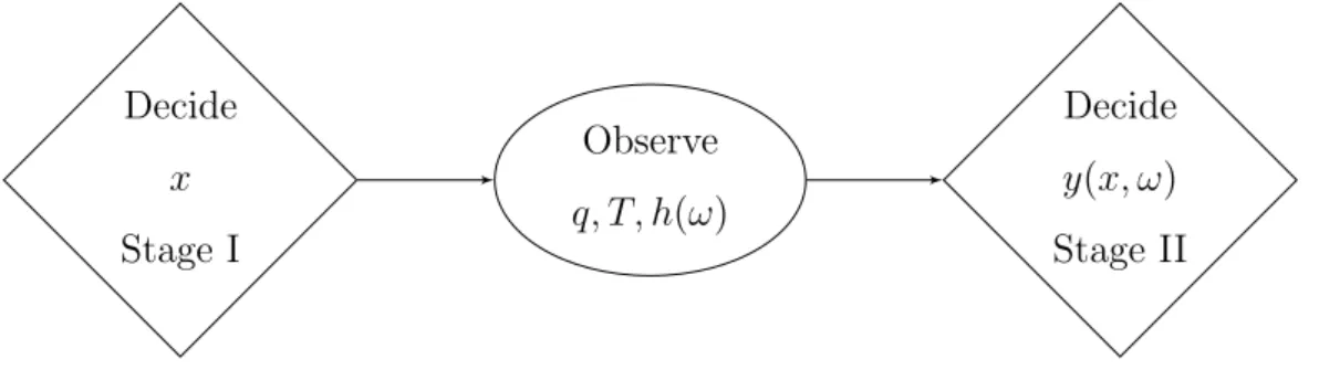
Thus, the information constraints are modified in such a way that the here-and-now or first-stage decisionsx are followed by the wait-and-see or second-stage decisions y = y(x, ω), carried out after the randomness is observed. These decisions are governed by the fixed recourse9 _matrix _W _{and penalized}

withrecourse costs q(ω) to enter the objective function. Then, we get the two-stage information scheme of alternating decision and observation depicted in Figure 3.2. This scheme can be naturally extended to a multistage framework involving sequential decisions for situations where randomness is subsequently revealed over time, cf. [SDR09], [Pr´e95].

Decide x Stage I Observe q, T, h(ω) Decide y(x, ω) Stage II

Figure 3.2: Information Constraints

In the present work, we will restrict ourselves to the two-stage approach, which yields the formulation

” min ”    c(ω)>x+q(ω)>y : T(ω)x+W y=h(ω) x∈ X, y ∈ Y    , (3.6)

where X,Y are polyhedral sets possibly with integer requirements. The con-straints of this model are now posed for (IP-almost) all ω and hence are well-defined. The second-stage decisions y are solutions of a (parametric) linear program (LP) with the following value function

Φ(x, ω) := min y∈Y{q(ω)

>

y: W y=h(ω)−T(ω)x}. (3.7) The study of this function and its properties plays the key role in the theory of problems with recourse. The most widely studied problem in this class is

9_{The randomness of the recourse matrix may lead to extreme numerical instability for} discrete distributions, cf. [RS03, p. 80] and [BL97, pp. 109] for a more general view.

(41)

obtained if we minimize the expectation of the overall, i.e., of first- and second-stage, costs. For this purpose, we define the expected recourse function

QIE(x) :=IEωΦ(x, ω), (3.8) and get a so-called deterministic equivalent formulation10 _{of the expectation}

based stochastic program as min x∈X{c

>

x+QIE(x)}.11 (3.9)

Clearly, the program is well-posed, and if the function QIE was given, it would translate into a deterministic nonlinear program. In fact, if the second-stage problem (3.7) is solvable for at least onex, the function Φ(·, ω) is convex and even piecewise linear in the pure linear case, cf. [SDR09, Proposition 2.1]. Under certain assumptions, convexity results can also be transferred to the ex-pected recourse functionQIE, cf. [SDR09, Propositions 2.3, 2.7], which enables an efficient algorithmic treatment of the model (3.9) and hence contributes to the popularity of the mean-based approach.

3.1.3 Risk Aversion and Dominance Constraints

In what follows, we assume the two-stage framework with recourse presented above to be the modeling technique of choice, i.e., probabilistic constraints are assumed to be already included as linear constraints in the polyhedron X

containing all first-stage restrictions. Thus, it is assumed that the decisions we make will ensure feasibility of our model with a sufficient reliability level and in exchange for certain costs.

Staying in this framework, we now return to the treatment of optimality. To this end, we represent the overall cost for each first-stage decisionxas a rv

10_{The term}_{deterministic equivalent} _{implies that all symbols of rvs are eliminated in the} formulation. We will stick to this term though it may be misleading, because stochastic problems are deterministic regardless of their formulation, as was argued in [Pr´e95, p. 234]. 11_{For ease of exposition, we assume from this point onwards}_c₍_ω_{) =}_c_{to be deterministic.} Due to linearity of the expectation, here we could simply take the average of the values.

(42)

f(x, ω) :=c>x+ Φ(x, ω), (3.10) with Φ(x, ω) as in (3.7), and thus obtain the family (3.1) of rvs with the specific structure. Selecting the ”best” rv out of this family through taking the expectation of the costs, as it was done in the formulation (3.9), rests upon a risk neutral decision model and hence may lead to first-stage decisions incurring ruinous costs for unfavorable random outcomes.

A popular way to consider risk aversion consists in the application of a mean-risk optimization model that here takes the shape

min

x∈X IE(f(x, ω)) +λρ(f(x, ω)) (3.11) and was studied in [Ahm06], [Tie05] and [ST04] in more detail. If the risk functional ρ is λ-consistent with SD, a strict minimum of this model will be non-dominated in SD in view of (A.4) and (A.6). Being computationally at-tractive, this approach is thus justified on grounds of the decision theory.

However, a drawback of mean-risk models is the need to specify the risk aversion parameter λ directly or to employ a sensitivity analysis on this pa-rameter.12 _{To avoid this difficulty, SD-consistent mean-risk dominance, see}

(A.3) and (A.5), may be used instead. As a partial order, it yields the multi-criteria, here bi-multi-criteria, optimization problem

min

x∈X{IE(f(x, ω)), ρ(f(x, ω))} (3.12) with conflicting objectives. Such a problem is not likely to possess a solution that simultaneously optimizes each of the objectives. Hence, the set ofPareto optimal solutions, called theefficient frontier, can be considered.13 For (3.12), a solution ¯x ∈ X is Pareto optimal if there is no other x with f(x, ω) ≺IE,ρ

f(¯x, ω). Thus, these solutions will also be non-dominated w.r.t. SD.

12_{Because the risk measure itself is typically not given naturally, families of other risk} measures may have to be considered as well.

(43)

It is also possible to look for solutions preferable w.r.t. SD directly. Result-ing optimization problems then possess a continuum of objectives. Though for finite, discrete distributions the number of objectives can be reduced to a fi-nite number, cf. [Ogr02] and [RDDM06], such models remain relatively hard to solve. By contrast, if the utility function of the decision maker is given explic-itly, its optimization yields a computationally attractive risk-averse technique referred to as the Bernoulli principle, cf. [Pr´e95, pp. 221]. Unfortunately, this method is not universally applicable, as we have argued in Section 2.1.

In the present thesis, we will now concentrate on an alternative way to incorporate risk aversion through shifting its treatment to the constraints. This trick is well-known from deterministic programming with conflicting objectives, all but one of which can be transformed into goal restrictions.14

Here, this idea implies imposing constraints on the risk, thus defining deci-sions with ”acceptable” risk as feasible solutions. To ensure such ”economic” feasibility, probabilistic constraints and also ICC or constraints on risk mea-sures could be used, once corresponding data on probability and risk thresholds is available. Instead, in some practical situations areference random outcome Y- a so-calledbenchmark - is available. We will concentrate on such situations and look for decisions producing outcomes preferable to the benchmark.

The seminal model for this type of problems was proposed by Dentcheva and Ruszczy´nski in [DR03], [DR04a]. Inspired by applications in portfolio optimization where benchmarks naturally arise from stock indexes like [SP], the authors employed stochastic orders to characterize the preferable outcomes.

Thus, the following dominance-constrained model was obtained:

max{g(X) :Y(i)X, X∈ C}, (3.13)

where Y was the benchmark rv, C a convex and closed set and g a concave

14_{An intermediate approach is followed in the so-called}_{goal programming}_{where violations} of the goal restrictions are additionally penalized in the objective, cf. [CCF55]. However, this approach does not seem applicable here.

(44)

continuous functional. For dominance constraints of first and second order the feasible regions of this problem were shown to be closed, and for SSD even convex, cf. [DR03]. Moreover, under rather weak assumptions15it was shown in [DR04b] that problems with SSD constraints are convexifications of problems with first order constraints (which are not convex in general). For stability and sensitivity analysis of these problems the author refers to [DHR07] and [DR13].

In the framework of EUT, the dominance-constrained model (3.13) guar-antees the preference of the solution X by all decision makers with utility functions in the corresponding class Ui, see Definition 2.1.1. In particular, no risk-averse decision maker will strictly prefer the benchmark outcome over a feasible solution to the second order model.

Conversely, it was shown in [DR04b] and [DR03] that utility functions of EUT can be identified with Lagrange multipliers associated with the domi-nance constraints of (3.13). Moreover, dual representations of SD from Propo-sitions 2.2.6 and 2.2.10 possess Lagrange multipliers that can be identified with dual utility functions in the sense of RDEUT, cf. [DR05]. In this way, prob-lems with SD-constraints can be regarded as dual to EUT and RDEUT, thus providing a link between both theories.

Links to SD-consistent mean-risk and mean-risk dominance models exist, as we have already discussed above, because their optimal values yield feasible solutions for dominance-constrained problems. Due to the dual representations of SD, dominance constraints can be also viewed as continua of constraints on important risk measures. By Proposition 2.2.1 (ii), first order dominance constraints are nothing else than a continuum of probabilistic constraints. In view of Proposition 2.2.2 (ii) and (3.5), SSD constraints can in turn be viewed as a continuum of ICC.

Recent applications of dominance-constrained models include, e.g.,

finan-15_{E.g., for a discrete distribution of}_Y_{with equiprobable outcomes or if its distribution is} continuous, cf. [DR04b].

(45)

3.2. Stochastic Programming: Methods

cial optimization [DR06] and power generation capacity expansion problems [VBZE13]. For recent interesting theoretical developments we refer to contri-butions on multivariate SD [DR09, HdMM10, AL10], and on dynamic opti-mization models with dominance constraints [DR08, HJ13].

Finally, we introduce the problem class we will work with starting from Chapter 4. It results from the specialization of problem (3.13) for the cost minimization framework, where the decision dependent random outcome is given with f(x, ω) from (3.10). A typical problem of the relevant class then takes the shape

min{g(x) : f(x, ω)(i) d(ω), x∈ X } (3.14)

where(i) refers to the orders FSD and ICX, cf. (4.1). Thus, model feasibility

is assured through recourse actions, whereas the ”economic” feasibility of a decision is defined w.r.t. a cost benchmark d(ω) by means of the SD-rules. In this way, the model combines one of the most popular feasibility modeling techniques of SP with the decision theoretical benefits of SD.

Models of the form (3.14) were proposed in [GNS08, GGS07]. The special case with a linear second stage was considered in [DS10]. Applications were carried out, e.g., in energy trading [CGS09] and in operation planning of virtual power plants [DGG+_11].

Building up on these works, in the following we will develop appropriate solution techniques for this interesting but demanding problem class. Since our tailored methods are based on the standard methods of SP, we first outline their main ideas in the following section.

3.2 Stochastic Programming: Methods

3.2.1 Deterministic equivalents

A simple way to approach a two-stage stochastic program is to tackle its de-terministic equivalent formulation directly. For the mean-based problem, the

(46)

deterministic equivalent (3.9) can be written down as the linear program min      c>x+ L P `=1 π`q>y` : Ax=b, x≥0, T x+W y` =h`, y` ≥0, `= 1, . . . , L      (3.15) for a finite discrete distribution of the right-hand side with probabilitiesπ1, . . . , πL for the scenarios h1, . . . , hL. While we assume the recourse matrix W to be fixed for numerical reasons, cf. [RS03, p. 80], the matrixT and the cost vector

q will be presented as fixed only for the ease of exposition. Also the equality form of the stage constraints and the restrictions on first and second-stage variables are presented exemplary.16

To formulate risk-averse models as (mixed-integer) linear programs, aux-iliary (sometimes binary) variables and a so-called Big M, which is a large number associated with these variables, can be used. For example, under cer-tain assumptions, cf. [Tie05], there exists a constant M > 0, such that the pure risk problem min{V@Rα(x): x∈ X } can be equivalently restated as

min                  η: c>x+q>y`−M θ` ≤ η, ∀` T x+W y` = h`, ∀` L P `=1 π`θ` ≤ 1−α, x∈ X, η∈_R, y` ≥0, θ` ∈ {0,1} ∀`                  . (3.16)

With the help of the minimization rule (2.26), an analogous representation can be gained for the problem of CV@Rαminimization:

min          η+ ₁_−α1 L P `=1 π`θ` : c>x+q>y`−θ` ≤ η, ∀` T x+W y` = h`, ∀` x∈ X, η∈_R, y` ≥0, θ` ∈R+ ∀`          , (3.17)

cf. [Tie05] for more details on such equivalents and other risk measures. Clearly, MILP equivalents of mean-risk models directly arise as combinations of the mean-based problem (3.15) with a corresponding pure risk problem.

16_{More generally, the variables are assumed to be contained in nonempty closed convex} polyhedra, which arise as solution sets to systems of linear inequalities (later also involving certain integer requirements).

(47)

3.2. Stochastic Programming: Methods

In view of the close relations between V@Rαand FSD and CV@Rαand ICX, it is not surprising that formulations (3.16) and (3.17) have similarities with the MILP equivalents

min                  g>x: c>x+q>y`k−M θ`k ≤ dk ∀` ∀k T x+W y`k = h` ∀` ∀k L P `=1 π`θ`k ≤ K P j=k+1 pj ∀k x∈ X, y`k ≥0, θ`k ∈ {0,1} ∀` ∀k                  (3.18) and min                  g>x: c>x+q>y`k−θ`k ≤ dk ∀` ∀k T x+W y`k = h` ∀` ∀k L P `=1 π`θ`k ≤ K P j=k+1 pj(dj−dk) ∀k x∈ X, y`k ≥0, θ`k ≥0 ∀` ∀k                  , (3.19)

which were derived in [GNS08] and [GGS11] for the dominance-constrained problems

min{g>x:f(x, ω)(1) d(ω), x∈ X } (3.20)

and

min{g>x:f(x, ω)icx d(ω), x∈ X }. (3.21) Here, the objective function g(x) is assumed to be linear, and the distri-bution of the benchmark rvd(ω) is finite, discrete with scenariosd1, . . . , dKand probabilitiesp1, . . . , pK. We will discuss these so-calledlifting-representations17 in Chapter 4 in more detail also presenting some possible improvements and modifications. In Section 5.2, then the so-called polyhedral representation for the problem with ICX will be discussed. This representation avoids any aux-iliary variables and goes back to a representation obtained in [KH86] for ICC. Thus, a solution technique for risk-averse stochastic programs may consist in applying readily available efficient solvers, like [CPL13] and [GUR13], to

17_{This term was proposed by F´}_abi´_{an in [F´}_{ab12] to reflect the usage of auxiliary variables} which lift the problem dimension.

Models and algorithms for dominance-constrained stochastic programs with recourse