Individual and ensemble functional link neural networks for data classification

(1)

Individual and Ensemble Functional Link

Neural Networks for Data Classification

by

Toktam Babaei BSc. and MSc Physics

Submitted in fulfilment of the requirements for the degree of

Doctor of Philosophy

Deakin University

(2)

(3)

(4)

iii

Abstract

In artificial neural network (ANN) research, the functional link neural network (FLNN) is a well-known alternative to the standard feedforward ANNs such as the Multilayer Perceptron network. The FLNN has a flat structure, i.e., with no hidden layer(s), therefore reducing its structure complexity while retaining the capability of solving non-linear classification and regression problems. This research focuses on using different FLNN-based models to tackle data classification tasks. Firstly, an evolutionary-based modification to the FLNN, known as reduced-FLNN1 (rFLNN1), is proposed to optimise the network structure and improve its classification performance. Encouraged by the good performance of rFLNN1, another improved version, known as reduced-FLNN2 (rFLNN2), is proposed. The rFLNN2 model merges optimisation of both network structure and network weights into one search problem, in order to generate a parsimonious FLNN model with high classification capabilities. To further improve the robustness of rFLNN2 an ensemble of multiple rFLNN2-based models is formulated. Coupled with the behavioural knowledge space and a novel decision fusion method based on the ordered weighted averaging operator, the ensemble model is able to handle noise-corrupted data classification problems. Extensive experiments covering benchmark classification problems from the machine learning repository of the University of California, Irvine and KEEL-data set repository are performed to evaluate the effectiveness of the proposed rFLNN-based individual and ensemble models for data classification. In addition to benchmark data sets, two real-world problems are used for evaluation. The results are analysed, discussed, and compared with those published in the literature. The outcomes positively demonstrate the potential and efficacy of the proposed rFLNN-based models for undertaking data classification problems.

(5)

iv

List of Publications

T. Babaei, H. Abdi, C. P. Lim, and S. Nahavandi, "A study and a directory of energy consumption data sets of buildings," Energy and Buildings,vol. 94, 2015, pp. 91-99 T. Babaei, C. P. Lim, H. Abdi, and S. Nahavandi, "A Modified Functional Link Neural Network for Data Classification," in Emerging Trends in Neuro Engineering and Neural Computation, ed: Springer, 2017, pp. 229-244

I. Hettiarachchi, T.Babaei, T. Thi Nguyen, C.P. Lim, S. Nahavandi, "A fresh look at functional link neural network for motor imagery-based brain-computer interface" , J. of Neuroscience Methods, (Accepted with minor revisions)

(6)

v

Acknowledgment

I am sincerely grateful to my advisors Saeid Nahavandi, Chee Peng Lim, and Hamid Abdi, who are brilliant researchers and amazing persons. I am deeply thankful to my principal supervisor Saeid Nahavandi for his continues supports and encouragements. I would also like to express my deepest gratitude to my co-supervisor Chee Peng Lim, who will always remain a source of inspiration to me. His enthusiasm along with the knowledge and patience with which he approaches problems and builds insights make him an ideal advisor to have. I would also like to thank my other co-supervisor Hamid Abdi for his supports and for sharing his knowledge with me.

I am grateful to my family and friends for being a constant source of encouragement and motivation. Most of all, I would like to thank my parents for fostering in me the love of learning and discovery and encouraging me to follow my heart.

(7)

vi

List of Figures:

Figure 1.1: Summary of the relationship of research methodology... 5

Figure 1.2: Overview of research methodology ... 7

Figure 2.1: Schematic representation of a real neuron ... 9

Figure 2.2: Representation of an artificial neuron-single perceptron, w0 indicates the threshhold value of the perceptron ... 9

Figure 2.4: A schematic diagram of an MLP with two hidden layers, with h1 neurons in the first hidden layer and h2 neurons in the second hidden layer ... 10

Figure 2.5: The backpropagation algorithm for training the MLP network ... 11

Figure 2.6: Schematic diagram of FLNN ... 13

Figure 2.7: Pseudo code for standard GA algorithm ... 26

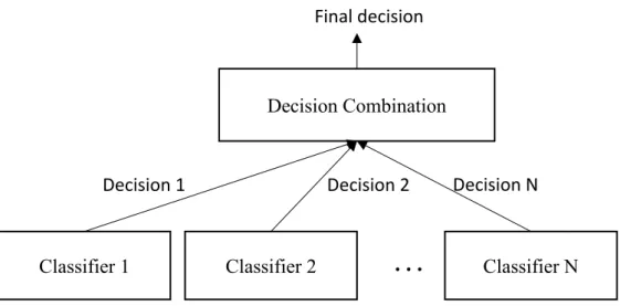
Figure 2.8: Schematic representation of an ensemble classification system. Decisions from individual classifiers are combined to generate the final decision ... 29

Figure 3.1:Structure of FLNN models with different basis functions used in this work ... 39

Figure 3.2: Pseudo code for FLNN ... 40

Figure 3.3: Data representation of circle-square classification problem (left), same problem in {𝑥₁2, 𝑥₂2} space (right)... 44

Figure 3.4 : A chromosome and corresponding network in rFLNN1 ... 44

Figure 3.5:Algorithm description of rFLNN1 ... 45

Figure 3.6: Topology of the rFLNN1 model ... 46

Figure 3.7:Topological structure of rFLNN2... 47

Figure 3.8: A chromosome and corresponding network in rFLNN2 ... 48

Figure 3.9: Cross over in rFLNN2 and the two resulted children ... 49

Figure 3.10:The first scenario of mutation in rFLNN2 system; the mutation point was selected from the binary part ... 49

Figure 3.11: Overview of ensemble classification system with rFLNN2 individual classifiers and BKS combination method ... 50

Figure 3.12: Quantifier functions "all"(𝑄_∗(𝑟)) and "any" (𝑄∗_{(𝑟)) ... 55}

Figure 3.13: Exploiting weights from a quantifier function ... 55

Figure 3.14: Steps to make final decision using the support value of an alternative given by m agents, using the OWA aggregation operator, where OWA weights are calculated using the quantifier function, Q. ... 57

(11)

x

Figure 3.16: Schematic diagram of operation phase in BKS-OWA ensemble model.𝜑_3 indicates the degrees of membership to each class (Section 2-7) ... 60 Figure 4.1: Schema of k-fold cross validation ... 71 Figure 4.2: Test accuracies of FLNNs with 4 different basis functions on 12 benchmark data sets... 75 Figure 4.3: Average of average accuracies with different noise placements in train and test sets respectively ... 79 Figure 4.4: True class labels and class predictions by Poly-,Tr-,Le-,and Ch- FLNN classifiers for 67 test samples of Ecoli problem in a fold ... 80 Figure 4.5: Schematic diagram of HFLNN proposed in [32] vs. rFLNN1 with the same basis functions ... 81 Figure 4.6: Performance comparison (bottom) with respect to maximum training accuracy (top) ... 84 Figure 4.7: Fraction of discarded expanded features ... 85 Figure 4.8: Percentage of weights in rFLNN2 and EFLNN models compared to that in

original FLNN ... 88 Figure 4.9: 5-fold classification accuracy results for clean train –noisy test datasets ... 92 Figure 4.10: 5-fold rejection rate results for data sets with different clean and noisy

configurations. ... 92 Figure 4.11: Schematic diagram of fault detection and diagnosis (adapted from [182]) ... 100

(12)

xi

List of Tables

Table 2.1: Common activation functions used in ANNs ... 10

Table 2.2: Comparison of computation complexity between FLNN and an L-MLP layer in one iteration with BP algorithm (adapted from [67]) ... 15

Table 2.3: Summary of studies reviewed in this section ... 18

Table 2.4 Summary of papers on Evolutionary feature selectionation ... 25

Table 2.5: Summary of papers on Ensemble classification methods... 33

Table 3.1: A general BKS table associated with a three-classifier model for a binary classification problem (Nunits= 23) . 𝑁1𝑈1 is the number of training samples with the received predictions according to the combination of unit 1, that their true class label is c1. . 52

Table 4.1: Summary of the benchmark data sets employed in the experimental study ... 69

Table 4.2: Look up table for the two-tailed sign test at 0.05 and 0.1 levels of significance [180] ... 72

Table 4.3: Test Accuracies of FLNN classifiers with different basis functions, over 5-fold dataset taken from KEEL repository... 73

Table 4.4: Statistical sign test results for significance levels of α=0.05 and α=0.1. ... 74

Table 4.5: Average test accuracies and standard deviations for data with 20% level of noise in training data and clean test ... 76

Table 4.6: Pairwise comparison of FLNN classifiers based on their performance over 12 data sets, using two tailed sign test ... 76

Table 4.7: Average test accuracies for data with clean train and 20% level of noise in test data ... 77

Table 4.8: Pairwise comparison of FLNN classifiers over 20% level of noise in train-clean test problems ... 78

Table 4.9: Average test accuracies for data with 20% level of noise in both training and test data ... 78

Table 4.10: Pairwise comparison of FLNN classifiers for 20% of noise in train and test data, using two tailed sign test with α=0.05, and 0.1 level of statistical significance ... 79

Table 4.11: Performance (2-fold cross validation test accuracy) comparison of proposed rFLNN1 and three other models with eight benchmark data sets ... 83

Table 4.12:Comparative performance study w.r.t. maximum train accuracy / test accuracy . 85 Table 4.13:Comparative results of rFLNN2 ... 87

(13)

xii

Table 4.14: Five folds cross validation accuracy of rFLNN2 ensemble with normal BKS and with BKS-OWA combination systems - results for clean datasets five folds ... 89 Table 4.15: Five folds cross validation accuracy of rFLNN2 ensemble with normal BKS and with BKS-OWA combination systems- results for noisy train –clean test datasets ... 89 Table 4.16: Five folds cross validation accuracy of rFLNN2 ensemble with normal BKS and with BKS-OWA combination systems- results for clean train –noisy test datasets ... 90 Table 4.17: Five folds cross validation accuracy of rFLNN2 ensemble with standard BKS and with BKS-OWA combination systems for noisy train-noisy test datasets ... 90 Table 4.18: Test accuracy of rFLNN2 ensemble with BKS-SB BKS- OWA systems. The higher performance for each problem is bolded. ... 93 Table 4.19: Comparison of classification accuracies obtained for proposed ensemble model with eight other Ensemble classifiers ... 97 Table 4.20: Pairwise comparison of rFLNN2 ensemble with BKS-OWA system. The

rFLNN2 ensemble with BKS-OWA is α- level significantly better than other system

considering the cases it performed better on the 12 cases ... 98 Table 4.21: Summary of key characteristics of the Power quality dataset ... 99 Table 4.22: rFLNN2 ensemble with Standard BKS and with BKS-OWA combination

systems- results for power quality monitoring problem ... 99 Table 4.23: Summary of key characteristics of the induction motor fault diagnosis dataset 100 Table 4.24: rFLNN2 ensemble with normal BKS and BKS_OWA combination systems -results for four motor faults diagnosis problem ... 101

(14)

xiii

List of Abbreviations

AI Artificial Intelligence

ANN Artificial Neural Network

BKS Behavioural Knowledge Space

BP Back Propagation

DCS Dynamic Classifier Selection

DES Dynamic Ensemble Selection

EA Evolutionary Algorithm

FLNN Functional Link Neural Network

FNFN Functional Neural Fuzzy Network

GA Genetic Algorithm

HONN Higher Order Neural Network

HS Harmony Search

MA Memetic Algorithm

MCR Measure of Competence Based on Random classification

MCS Multiple Classifier Systems

MCSA Motor Current Signature Analysis

MFS Multiple Feature Subset

MLP Multi-Layer Perceptron

NMC Nearest Mean Classifier

NNE Neural Network Ensembles

OWA Ordered Weighted Averaging

rFLNN reduced Functional Link Neural Network

(15)

xiv

SLP Single Layer Perceptron

SVM Support Vector Machines

RVM Relevance Vector Machines

(16)

Introduction

This chapter starts with the preliminaries of artificial intelligence (AI) and artificial neural networks (ANNs). It then presents the motivations for using the functional link neural network (FLNN) for data classification, which is the main research focus of this thesis. A discussion on the development of ensemble models for data classification is provided. The research objectives and research methodology are explained. The thesis outline is described at the end of this chapter.

1.1 Artificial Intelligence

The recognition of AI as an important research domain dates back to 1956[1]. The term AI broadly refers to how a machine emulates the "cognitive" functions of the human brain, such as "learning" and "problem solving", and uses them to operate autonomously in complex, changing environments. In general, AI encompasses a number of machine learning methodologies. They cover conventional statistics, neural computing, evolutionary computing, and fuzzy computing models, to name a few [2]. The artificial neural network (ANN) is one of key data-based learning AI methodologies.

In general, learning techniques can be divided into three categories: supervised learning, unsupervised learning, and reinforcements learning [1]. Supervised learning establishes a mapping function from a training set containing input-output data pairs. Regression and pattern classification are supervised learning tasks, which comprise continuous and discrete outputs, respectively. Data (pattern) classification is concerned with building machines to classify data samples based on either a priori knowledge, or statistical information extracted from data samples [3-5]. A classical definition of pattern is an entity that can be represented by a set of attributes (a feature vector) [6]. As an example, a pattern can be an audio signal, where the corresponding feature vector is its frequency spectral components; or a patient, where the feature vector is the results of his/her medical tests. This thesis is focused on data classification problems with supervised ANN models.

(17)

2

1.2 Data classification and Artificial Neural Networks

Data classification is a key task in accomplishing many activities. Accordingly, many studies have been devoted to developing methods from different principles to solve data classification problems. One of the earliest investigations is from the statistics community. Fisher [7] proposed a linear discriminant function to tackle data classification problems. It was later extended to a quadratic form[8]. Bayesian theory is another fundamental statistical method used in devising various data classification methods [9, 10]. While these statistical principles have certain limitations with respect to the underlying statistical assumptions [11, 12], they provided the necessary basis for further research. In addition to statistical principles, a variety of AI-based models have been researched for data classification, e.g. rough sets, fuzzy sets, decision trees, k-nearest neighbors, and support vector machines (SVM).

Among different learning methodologies, ANNs are popular AI-based data learning models. Indeed, research interest in ANNs stems from two aspects: (i) to understand and model mathematically the biological nervous system in humans; (ii) to develop intelligent learning systems that mimic the way how humans perform certain tasks, such as capturing data and interpreting information. This research is concerned with the data learning aspect of ANNs, in view of the potential impact of such learning models in undertaking data classification problems in the real environments.

ANN emerges as useful data processing models [13]. To date, there are a number of different ANN models, which include the Multi-Layer Perceptron (MLP) network [14] , Hopfield network [15, 16], and Radial Basis Function (RBF) network [16]. These models have been used as a promising method to support and improve human decision-making in different areas, e.g. function approximation [17-19], rule extraction [20], forecasting and prediction [21, 22], business [23, 24], engineering [25], and medicine [26]. An ANN requires knowledge through a learning process. It simulates the inter-neuron connection strength as weights to store knowledge [30]. As a result, it has unique characteristics including the ability to learn the relationships between inputs and output data pairs for tackling data classification problems.

(18)

3 1.3 Problem statement and motivations

One of the popular ANN models is the Multilayer Perceptron (MLP). The input layer in an MLP consists of units (neurons) equal in number to the input features and one bias unit. The output layer consists of units equal in number to the output classes (labels). It has one or more hidden layers in between the input and output layers. The role of the hidden units is to provide the MLP with the capability of handling non-linear input-output mapping. It has been shown that an MLP with a suitable architecture is able to approximate (or learn) any nonlinear decision boundary [27]. Training the MLP includes finding the appropriate weights. The most common training method is the back-propagation (BP) learning algorithm.

There are a number of issues in designing and developing an efficient and effective learning algorithm for the MLP network, which include local minima, saturation, weight interference, initial weight dependence, and overfitting. On the architecture side, the issues include how to determine the number of hidden layers and the number of hidden units in an MLP network. All these learning and architecture issues present great impacts on the usability and usefulness of the MLP in tackling real-world problems. As such, a straight forward way to avoid some of the key problems is to remove the hidden layer(s), which would compromise the ability of an MLP to capture nonlinear input-output relationships. However, studies have been shown that if higher order neurons (also known as sigma-pi neurons [28]) are added to the original neurons in the input layer, an MLP network without any hidden layers could retain its nonlinearity ability. This is the main idea behind the research on higher order neural networks (HONNs) [29], [30]. HONNs have appeared as an attractive alternative to eradicating some of the MLP limitations. In this respect, the functional link neural network (FLNN) poses as a class of HONNs that utilizes a function of the original inputs to enhance the inputs [30]. In an FLNN, the hidden layers are removed and the network complexity is reduced, resulting in a straightforward architecture and a straightforward learning process. These advantages make FLNN attractive for researchers in the field [31-36], as the FLNN model alleviates the key issue in determining the network complexity (the number of hidden nodes and hidden layers) and the associated learning process of a standard MLP network, which is the building block of deep learning models. In an FLNN, the number of enhanced inputs is determined by the set of basis functions, and leaning can be framed in the form of a quadratic optimization [37]. Moreover, a standard MLP network is not efficient in dealing with dynamically changing

(19)

4

environment which require an on-line learning capability. In this aspect, FLNN-based models have been successfully used in undertakings on-line learning problems [37].

The design and development of FLNN-based learning models with the capability of handling various data classification problems constitutes the main aim of this research. The resulting models are evaluated using a variety of benchmark and real-world classification data sets. On the other hand, studies have been shown that ensemble models, in which the predictions from multiple classifiers are combined using a suitable decision combination method, can generate more accurate decision for each input, therefore improving the overall classification performance [38]. In this respect, majority voting is a straightforward strategy to combine the decisions from an ensemble of individual classifiers. Other elaborated schemes are also available to aggregate individual decisions, e.g. the behaviour knowledge space (BKS) method. The BKS can efficiently aggregate decisions of individual classifiers to deliver better results [39]. While the BKS can be used as an effective component in an ensemble model, it has some limitations. The major limitation with the BKS is its rejection rate. When the BKS fails to give a prediction for an input sample, due to lack of confidence, the input sample is rejected [40-42]. This issue becomes serious when noisy data samples are available. Therefore, this research investigates the use of an aggregation operator to tackle the rejection problem of the BKS in an ensemble model.

1.4 Research aim and objectives

The main aim of this research is to formulate a framework that utilizes the FLNN-based models as a useful and usable ensemble system for undertaking complex data classification problems. The specific research objectives are as follows:

1. to enhance the FLNN by optimising its network architectures and overcoming issues related to curse of dimensionality using evolutionary methods;

2. to improve the classification performance by devising an ensemble system consisting of different individual FLNN-based models

3. to adapt an aggregation operator to effectively combine the predictions from multiple individual FLNN-based models in the ensemble system

4. to apply the resulting individual and ensemble models to complex and noisy data classification problems.

(20)

5 1.5 Research methodology

A systematic, step-by-step methodology is adopted in this research. The focal point lies on investigating the FLNN capability of handling complex and noisy data classification problems. Firstly, different ANN and FLNN models proposed in literature are surveyed, in order to provide a comprehensive understanding pertaining to the current advances in the ANN and related domains. Besides that, understanding the properties and limitations of the existing ANN and related models is important, so that appropriate methods to tackle them can be formulated.

By analysing different methods, data classification models using FLNN and complementary methods are devised. Systematic and comprehensive empirical studies are carried out to evaluate and ascertain the usefulness of the developed models. Figure 1.1 shows a summary of the research methodology adopted in this research.

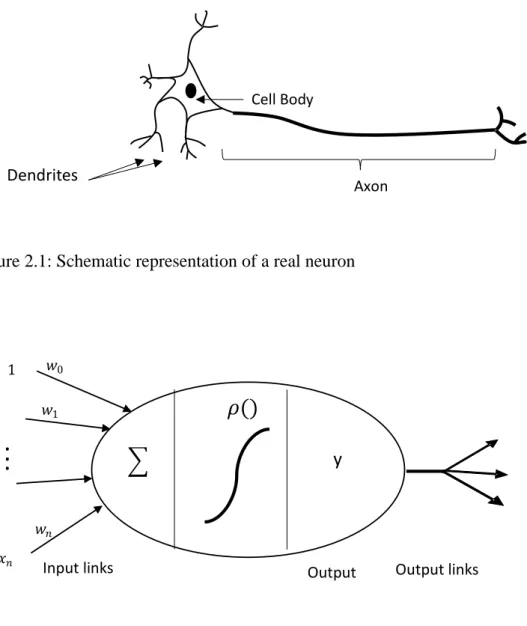
Figure 1.1: Summary of the relationship of research methodology

In this research, the key activities to achieve the research objectives are as follows: Key goal: An FLNN-based framework for undertaking

complex and noisy data classification problems

Key objective: To enhance the FLNN classification capabilities by formulating an ensemble model comprising different individual FLNN models

Key research question: How to devise effective FLNN learning algorithms and decision combination

algorithms for data classification using multiple FLNN-based models?

(21)

6

Activity 1. The FLNN classifier is thoroughly examined, in order to identify the existing limitations, particularly the curse-of-dimensionality problem. This results in a parsimonious FLNN model with reduced architectural complexity, known as rFLNN1.

Activity 2. The performance of rFLNN1 is evaluated comprehensively using benchmark data sets, and the results are compared with those of other models reported in the literature. Activity 3. An enhanced FLNN-based model using an evolutionary method, known as rFLNN2, is proposed. Both network architecture and weight tuning are combined as optimization problem, which is solved using the evolutionary method.

Activity 4. The performance of rFLNN2 is evaluated comprehensively using benchmark data sets, and the results are compared with those of other models reported in the literature. Activity 5. An ensemble system to tackle the problem of combining multiple predictions from individual FLNN-based models with different expansion functions is formulated. An effective aggregation operator is formulated for the ensemble system.

Activity 6. The performance of the ensemble model is comprehensively evaluated using benchmark noisy data sets, and the results are compared with those of other models reported in the literature. In addition, real-world data sets are used to ascertain the applicability of the ensemble system in undertaking real data classification problems.

Figure 1.2 summarises the key activities of this research.

1.6 Outline of the thesis

The outline of the rest of this thesis is as follows. Chapter 2 contains the background and literature review related to ANNs and FLNN-based models as well as complementary methods such as evolutionary algorithms and ensemble methods. The detailed dynamics of the proposed rFLNN models and the ensemble system are presented in Chapter 3. A comprehensive experimental study with benchmark and real-world data sets is presented in Chapter 4. The results are analysed, compared, and discussed thoroughly. Finally, conclusions and suggestions for further research are presented in Chapter 5.

(22)

7 Figure 1.2: Overview of research methodology

Activity 1

• Enhamcing the FLNN model by reducing its architectural complexity, resulting in rFLNN1

Activity 2 • Evluating the performance of rFLNN1 using benchmark problems

Activity 3

• Improving rFLNN1 by combining both network architecture and weight tuning as an optimisation task , resulting in rFLNN2

Activity 4 • Evaluating the performance of rFLNN2 using benchmark problems

Activity 5 • Devising an ensemble system with multiple individual FLNN-based models

Activity 6

• Evaluating the performance and applicability of the ensemble system with benchmark and real-world data classification problems

(23)

8

Background and Literature Review

As described in the first chapter, the focus of this thesis is on investigating the efficiency of ANNs, particularly FLNN-based models, for data classification. The evolutionary computing and ensemble methods are adopted. A linguistic aggregation operator, i.e., ordered weighted average (OWA), is also used to combine multiple decisions in ensemble framework. As such, this chapter provides the related background ANN, FLNN, evolutionary networks, ensemble methods, and OWA operator as the linguistic aggregation operator is defined in this framework. A critical review on the corresponding literature is also presented.

In the first section, the general standard MLP is described. Then the fundamental theory of FLNN is presented. A review on the related publications in the literature is provided. The review covers different FLNN variants and different applications. The next section deals with evolutionary models, in which various evolutionary algorithms (EAs) to optimise ANNs are reviewed. Then, a review on classification ensemble methods, with the focus on the ANN-based ensemble models is presented.

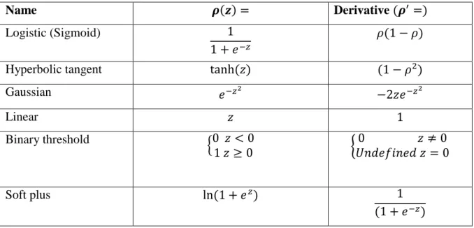
2.1 Overview of Artificial Neural Networks

ANNs offer an important paradigm for approximating nonlinear decision boundaries in classifying data. Being a black-box, they serve as valuable candidates when no appropriate physical/mathematical models exist for complex data classification tasks. An ANN in general consists of several processing units known as artificial neurons. These neurons are connected together according to a topology to form a network that mimic the biological neurons of human brain [43] . Figures 2.1 and 2.2 depict the biological neuron and its artificial counterpart. The first mathematical model of an artificial neuron was proposed by McCulloch and Pitts in 1943 [13]. Then, Rosenblatt in 1957 [44] refined the artificial neuron, and devised the so-called perceptron [45]. Equation (2-1) shows the mathematical model of an artificial neuron

𝑦 = 𝜌(∑𝑛𝑖=0𝑥𝑖𝑤𝑖) (2-1)

where the input features, {1, 𝑥1, 𝑥2, … , 𝑥𝑛}, are multiplied by the respective weight coefficients

(24)

9 Figure 2.1: Schematic representation of a real neuron

Figure 2.2: Representation of an artificial neuron-single perceptron, w0 indicates the threshhold value of the perceptron

The summation result passes through an activation function ρ(.) to generate the output of the perceptron. The function output can be the final output, or can be an input to another perceptron. The activation function determines the properties of the artificial neuron. Table 2.1 shows the common activation functions and their derivatives for ANNs. Among them, the unipolar logistic (sigmoid) function and hyperbolic tangent (𝑡𝑎𝑛ℎ) are used frequently as an activation function [45].

Axon Cell Body

Dendrites

Input links _Output Output links

𝑤_𝑛

𝜌()

𝑤₀ 1 𝑥𝑛 𝑤1

.

. .

y

(25)

10 Table 2.1: Common activation functions used in ANNs

Name 𝝆(𝒛) = Derivative (𝝆′₌₎

Logistic (Sigmoid) 1

1 + 𝑒−𝑧

𝜌(1 − 𝜌)

Hyperbolic tangent tanh (𝑧) (1 − 𝜌2)

Gaussian _𝑒−𝑧2 _−2𝑧𝑒−𝑧2 Linear 𝑧 1 Binary threshold _{0 𝑧 < 0 1 𝑧 ≥ 0 { 0 𝑧 ≠ 0 𝑈𝑛𝑑𝑒𝑓𝑖𝑛𝑒𝑑 𝑧 = 0 Soft plus ln (1 + 𝑒𝑧) 1 (1 + 𝑒−𝑧₎

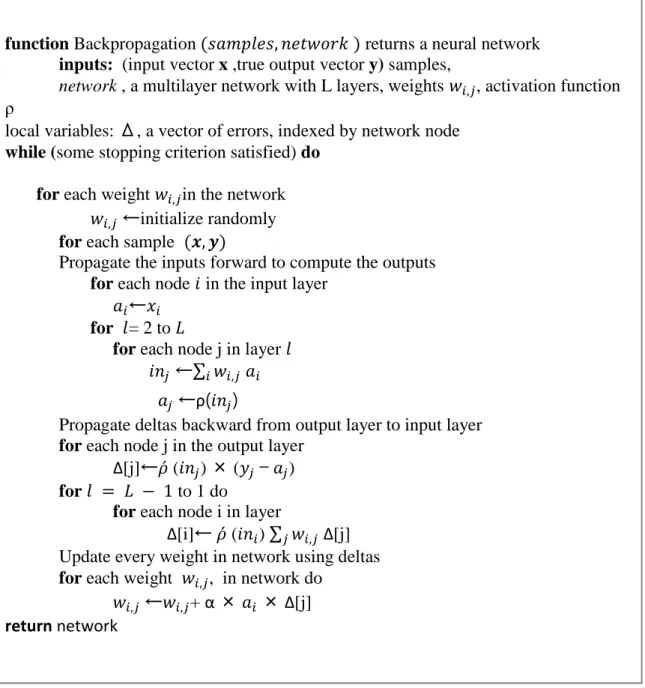
Figure 2.3 shows how a number of perceptron are organised in a network-like structure to form the so-called Multi-Layer Perceptron (MLP). The key learning procedure of an MLP is the back-propagation algorithm, which is summarised in Figure 2.4.

Figure 2.3: A schematic diagram of an MLP with two hidden layers, with h1 neurons in the first hidden layer and h2 neurons in the second hidden layer

Inputs First hidden layer Second hidden layer Outputs

.

𝑥2 𝑥𝑛 𝑦 1 𝑦 2 𝑥1

.

_.

.

𝑣1 𝑢ℎ1 𝑣ℎ2 𝑢1

(26)

11

Figure 2.4: The backpropagation algorithm for training the MLP network

Despite many successful applications of the MLP in function approximation and classification tasks, one of the problems is the plateaus error surface of the MLP [46, 47]. This is because gradient decent, as well as other training methods which are based on standard numerical optimization techniques, is susceptible to local minima of the error surface. The local minima trap poses a severe obstacle when the MLP is used to approximate complex functions. In approximating complex functions, the MLP architecture could grow to thousands of neurons, which makes the training process a difficult one.

function Backpropagation (𝑠𝑎𝑚𝑝𝑙𝑒𝑠, 𝑛𝑒𝑡𝑤𝑜𝑟𝑘 ) returns a neural network inputs: (input vector x ,true output vector y) samples,

network , a multilayer network with L layers, weights 𝑤_𝑖,𝑗, activation function ρ

local variables: Δ, a vector of errors, indexed by network node while (some stopping criterion satisfied) do

for each weight 𝑤_𝑖,𝑗in the network 𝑤_𝑖,𝑗←initialize randomly for each sample (𝒙, 𝒚)

Propagate the inputs forward to compute the outputs for each node 𝑖 in the input layer

𝑎𝑖←𝑥𝑖

for 𝑙= 2 to 𝐿

for each node j in layer 𝑙 𝑖𝑛_𝑗 ←∑ 𝑤_𝑖 _𝑖,𝑗 𝑎_𝑖

𝑎_𝑗←ρ(𝑖𝑛_𝑗)

Propagate deltas backward from output layer to input layer for each node j in the output layer

Δ[j]←𝜌 (𝑖𝑛𝑗) × (𝑦𝑗 − 𝑎𝑗)

for 𝑙 = 𝐿 − 1 to 1 do

for each node i in layer

Δ[i]← 𝜌 (𝑖𝑛_𝑖) ∑ 𝑤_𝑗 _𝑖,𝑗Δ[j] Update every weight in network using deltas for each weight 𝑤_𝑖,𝑗, in network do

𝑤_𝑖,𝑗←𝑤_𝑖,𝑗+ α× 𝑎_𝑖 ×Δ[j]

(27)

12

To alleviate the local minima problem some modification to the standard BP was proposed [48-50]. However a more recent method to deal with local minima is to use stochastic and heuristic optimisation methods [47]. Evolutionary algorithms (EAs) are heuristic optimization methods inspired by different mechanisms in natural evolution of organisms [51]. Mechanisms such as mutation, reproduction, and recombination are introduced to help EAs in searching large and high dimensional.

Another problem is that finding the appropriate MLP structure for a given task is not easy. The MLP performance strongly depends on whether it has an adequate structure to model the underlying data distribution. A small network structure may not be able to learn the underlying problem properly, while an excessively large network may over-fit training data as geometrically demonstrated in [52]. An over-fitted network lacks the generalization ability and fails to perform well on new instances. In fact, there is no theory that governs finding the optimum MLP structure, making it a tedious trial-and-error process [53].

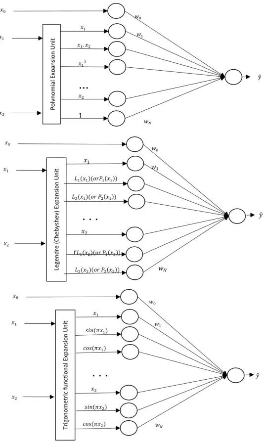
2.2 Functional Link Neural Network (FLNN)

As proposed by Klassen and Pao [12], the FLNN can be used for data classification and prediction tasks with a faster convergence speed and a lighter computational load as compared with the MLP network. This is because that the FLNN has a structure without any hidden layers, in contrast to the stacked structure of the MLP network. Although the FLNN model has only one layer of trainable weights, it is able to undertake non-linear classification and regression problems. This is owning to the functional expansion units embedded in the FLNN. These functional expansion units (or nodes) effectively enhance the input features by expanding them into a higher dimensional space, allowing the boundary (either linear or non-linear) to be approximated by hyperplanes in the expanded feature space [12].

The general topological structure of a single input- single output FLNN is shown in Figure 2.5. The FLNN consists of two parts: a transformation part and a learning part. In the transformation part, which includes the functional expansion block, each input is expanded to several terms using the expansion function. Denote each input pattern as:

𝑥 = [𝑥₁, 𝑥₂, . . . , 𝑥_𝑛] ∈ 𝑅𝑛 _(2-1)

(28)

13

dimensional space by expanding each element of the input vector to (𝐹 + 1) secondary features using a set of basis functions that can be represented as follows:

𝜑(𝑥_𝑖) = [𝜑0(𝑥𝑖), 𝜑1(𝑥1), … , 𝜑𝐹(𝑥𝑖)] (2-2)

where 𝐹 is the number of expansion terms.

Figure 2.5: Schematic diagram of FLNN

The set of expansion functions perform as the basis of the enhanced space. As such, they must be a subset of some orthogonal functions, {𝜑}𝜖ℒ(𝐴) , and hold the following

characteristics [54, 55]:

– 𝜑₀ is a linear function

– 𝜑_𝑖, 2 ≤ i ≤ n are linearly independent functions

– 𝑠𝑢𝑝_𝑛(∑𝑛 (‖𝜑_𝑖||)2 _{< ∞}

𝑖=2

Trigonometric functions, power polynomial functions, Chebyshev polynomial functions, Hermite polynomial functions , Legendre polynomial functions are some common orthogonal functions that can be used in the FLNN[56]. Finally the FLNN generates an output by applying an activation function ρ to the weighted sum of the expanded inputs, as follows:

Inputs Output 𝑥1 𝑦 1 𝑥0

.

Expan

sion Unit

𝑤0 𝑤_𝑁 𝑤1 𝜑1(𝑥1)

. .

.

. . .

𝜑𝑛(𝑥1)

(29)

14

𝑦 _𝑗 = 𝜌(𝑧_𝑗) ( 2-3 )

𝑧_𝑗 = ∑𝑁_𝑖=1𝑤_𝑗𝑖𝜑_𝑖(𝑥) ( 2-4)

where 𝑤_𝑗 = [𝑤_𝑗1, 𝑤_𝑗2, … , 𝑤_𝑗𝑁] is the weight vector associated with the 𝑗th output. Similar to the MLP, different types of activation functions can be applied to the weighted sum to generate the final output of the FLNN. The flat architecture of FLNN results in that only 𝑤_𝑗 are need to be learnt, and learning can be carried out rapidly in the form of quadratic optimization [37].

Computational Complexity

A discussion on computational complexity between an FLNN and an L-layer MLP network, both trained with the BP algorithm is presented. Considering that the L-layer MLP has 𝑛_𝑙 number of nodes in layer l, where l=1,…,L , and 𝑛₀ and 𝑛_𝑙 are the number of inputs and outputs, respectively. The computation that needs to be accomplished to update the weights of the MLP include addition, multiplication, and computation of tanh(. ). In case of the FLNN, computation of 𝜑𝑖 functions is also included. The computation steps in the MLP network are

as follows [57]:

– Forward calculation to find the activation value of all nodes of in the network ; – Back error propagation for calculation of square error derivatives;

– Updating of the weights of all the links in the network.

As such, the total number of weights to be updated in one iteration in the MLP is

∑𝐿−1𝑙=0(𝑛𝑙+ 1)𝑛𝑙+1.

In the FLNN, it becomes [57]:

𝑛₀+ 1,

It can be seen that as there is no hidden layer in the FLNN, the computational complexity is drastically reduced in comparison with that of the MLP. A comparison of computational load in one iteration for an MLP and an FLNN is summarized in Table 2.2.

(30)

15

In addition to a lower computational cost, the simpler structure of the FLNN means that it is less complex to combine the FLNN with an EA, and is less time consuming as compared with that of the MLP networks.

Table 2.2: Comparison of computation complexity between FLNN and an L-MLP layer in one iteration with BP algorithm (adapted from [57])

Operation MLP FLNN Addition 3 ∑𝐿−1𝑖=0𝑛𝑖𝑛𝑖+1+ 3𝑛𝐿− 𝑛0𝑛𝑙 2𝑛𝑙(𝑛0 + 1) + 𝑛1 Multiplication 4∑𝐿−1_𝑖=0𝑛_𝑖𝑛_𝑖+1+ 3 ∑𝐿_𝑖=1𝑛_𝑖 − 𝑛₀𝑛_𝑙+ 2𝑛_𝐿 3𝑛1(𝑛0+ 1) + 𝑛0 𝑡𝑎𝑛ℎ (. ) 𝑛𝑖 𝐿 𝑖=1 𝑛₁ 𝜑(.) --- 𝑛₀ On-Line Learning

Generally there are two main learning paradigms for neural networks, i.e., batch or off-line learning and incremental or onoff-line learning, in off-off-line learning scenarios the optimization process is conducted to update the knowledge base of the neural network with respect to the training data samples. While in online learning it attempts to update the knowledge base of the neural network incrementally as each training sample is presented [37].

Off-line learning, which normally consists of a training phase and test phase, is a widely used method in many neural networks including the standard MLP model. Once the training cycle is completed, the network is put into operation. Generally, no further learning is permitted when the network is in the operating mode, in order to preserve the learned knowledge base. The off-line learning paradigm is able to form an optimized knowledge base in the network structure. It is a viable method when the problem environment is stationary, and the training data samples are sufficiently representative of the problem [58]. However, when the network trained with off-line learning is presented with a previously unseen data sample, there is no built-in mechanism for the network to absorb the new information into its knowledge base on the fly. To absorb new information, the network normally needs to be retrained using the new

(31)

16

data sample together with all previous samples. On the other hand, online learning is able to deal with dynamically changing problems, e.g. stock price prediction [59] , sensory motor control [37] , and text mining [60]. In these applications, the learning period often varies according to the changing nature of the problem; therefore, the concept of ongoing learning is critically important. However, one major concern of online learning is the ability of the trained network to form an optimized knowledge base for tackling dynamically changing problems. This is a subject that has attracted a lot of attentions in neural network research. While the standard MLP model is not suitable for handling dynamic environments , the flat structure of FLNN and its quadratic optimization form of learning makes it one of the suitable candidates for on-line learning [37]. These works as well as other prominent works on FLNNs are reviewed in the next section.

2.3.2 Related Studies on the FLNN

A number of FLNN models have been proposed using various basis functions. They include the Chebyshev FLNN [18], Legendre FLNN (Le-FLNN), Hermite FLNN (He-FLNN), and Laguerre FLNN (La-FLNN). The Chebyshev FLNN (or Ch-FLNN) uses Chebyshev polynomials as the expansion block to enhance the inputs. Chebyshev polynomials, which come from solving the Chebyshev differential equations, make an orthogonal set of polynomials. The Ch-FLNN models have been successfully applied to system identification [61], function approximation [44], and digital communication [45] problems.

In [62], the FLNN was used to capture the dynamics and temperature–time dependent relationship of larva’s food in-take. It was shown that the FLNN yielded better results than several conventional models. Moreover, a sensitivity study revealed that the Legendre, Chebyshov, trigonometric functions performed better than Laguerre and Hermite functions [62].In a recent study [63], the FLNN models based on power polynomials, Laguerre, Legendre, and Chebyshev polynomials were devised. Their performances in financial time series forecasting were compared, with a term based on moving averaging calculation introduced in the expansion unit.

In [15], the gradient-based BP algorithm was replaced with a modified artificial bee colony algorithm to train the FLNN. The proposed FLNN variant was able to overcome the limitations of gradient decent, and achieve better classification rates, as compared with the original FLNN. In [16], Harmony search (HS) was integrated with the BP algorithm to improve

(32)

17

the learning capability of the original FLNN. In [17], the original FLNN was trained with another meta-heuristic algorithm, i.e., the firefly algorithm. The resulting FLNN was used for time series forecasting. The predictive accuracy and processing time were better than those from the original FLNN. In [18], an FLNN with a hybrid Particle Swarm Optimization (PSO)-BP learning algorithm for data classification was proposed. An improved version of this model was developed in succession [14]. The same group of researchers attempted to decrease the complexity and computational load of the FLNN by using a GA to select a subset of the input features from the original feature space [19].

A Functional Neural Fuzzy Network (FNFN) which uses the functional link neural network was proposed for solving classification problems in [64]. The FNFN model was able to construct its structure and adapt its parameters using an online learning algorithm. The online learning algorithm consisted of a structure learning procedure based on the entropy measure, while the parameter learning produce was based on the gradient-descent method [64]. Various simulation studies were conducted, and the results showed that FNFN performed better than other models in classification applications [64]. In [31] a nonlinear system control using a functional link-based neuro-fuzzy network (FLNFN) was presented. The online learning algorithm for the FLNFN model, which tackled both structure and parameter learning, was similar to that in [64]. The convergence analysis and universal approximation property of the FLNFN model were demonstrated in various simulations [31]. In [65] a random vector type of FLNN or RVFLNN was incorporated with convolutional network and CRVFL model was presented. This model was easy to train in contrast to other ANN model used for visual tracking. Moreover it was shown that by using a recursive least square approach the proposed in learning algorithm of the model, it can be updated online Various simulation on the visual tracking benchmark using this model showed its favorable performance against state-of–the-art methods, and an ensemble CRVFL also proved to be able to further improve the performance. In [66], an FLNN-based model was used to predict machinery noise in the mining industry. In [17], a benchmark study was conducted to compare an FLNN-based classifier against different common classifiers, including kNN (k- nearest neighbour), C4.5 decision tree, and the MLP. In [67], a model that combined the Radial Basis Function (RBF) network and Random Vector FLNN (RVFLNN) was presented. The proposed model could improve the recognition of words in an English script. In [66], the prediction capability of the FLNN was compared with several statistical models. For this purpose, the problem of predicting the

(33)

18

machineries noise in opencast mining, and some common standard noise forecasting models were examined. In [68], the FLNN with trigonometric basis function was adopted to handle multi-label classification problems. Enhancing the original input features to a higher order space helped to improve the separability of the class boundaries, and solved the major challenge in multi-label classification problems.

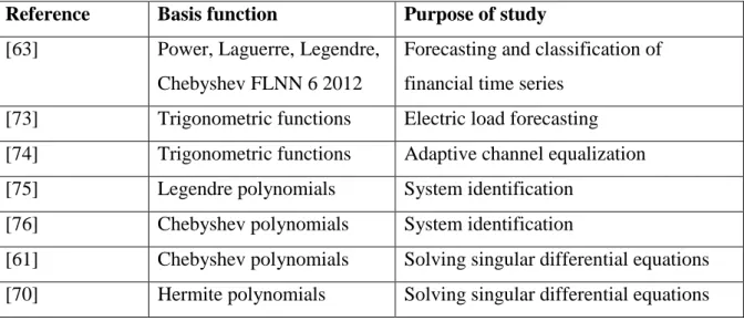
A few studies found the FLNN useful in solving differential equations, which are hard to solve using the existing mathematical methods. In [69], the FLNN with Chebyshev function expansion and the BP algorithm was used to solve a second order Lane-Emden type differential equation. The equation has singularity at the origin, which makes it challenging to find the answer function around this area. It was shown that Ch-FLNN was effective in solving both homogeneous and non-homogeneous Lane-Emden equations. In [70], the Hermite orthogonal polynomials were used as the expansion functions in an FLNN. The developed model was used to solve another differential equation known as Van der Pol-Duffing oscillator equation. Despite many advantage of the FLNN, some issues arise in real-world application of the FLNN. One key issue is related to the drastic increase of the number of expanded features, which leads to the “curse of dimensionality” [71] problem. As such, some studies addressed this problem by selecting an optimal set of original features, and then sending this smaller feature set to the functional expansion units for further processing [72]. Table 2.3 shows the summary of the works reviewed in this section.

Table 2.3: Summary of studies reviewed in this section

Reference Basis function Purpose of study [63] Power, Laguerre, Legendre,

Chebyshev FLNN 6 2012

Forecasting and classification of financial time series

[73] Trigonometric functions Electric load forecasting [74] Trigonometric functions Adaptive channel equalization [75] Legendre polynomials System identification

[76] Chebyshev polynomials System identification

[61] Chebyshev polynomials Solving singular differential equations [70] Hermite polynomials Solving singular differential equations

(34)

19

[77] Trigonometric functions FLNN model based on differential evolution and feature selection for noisy data

[78] Power Polynomials Evolution of functional link neural networks

[32] Trigonometric functions Hybrid GA-FLNN model for classification

[56] Chebyshev polynomials Improving the FLNN learning procedure using the PSO algorithm

[79] Trigonometric functions Improving the FLNN learning procedure using Harmony search algorithm

[80] Power polynomial Improving the FLNN learning procedure using Bee colony algorithm

[64] Trigonometric functions Adopting FLNN in a fuzzy network for handling online learning tasks

[31] Trigonometric functions An FLNN neuro-fuzzy network model for controlling a nonlinear system (on-line learning)

The curse-of-dimensionality problem of the FLNN constitutes the key motivation of this research to devise the rduced-FLNN1 (rFLNN1) and rFLNN2 models in Chapter 3. The rFLNN1 model uses the GA to optimize the number of neurons expanding to the output neurons. The rFLNN2 model takes the advantage of the simple structure of the FLNN, and uses the GA to find the optimal expanded feature set and network weights simultaneously. To achieve this, novel reproduction operators including crossover and mutation are introduced in Chapter 3. As such the next sections are dedicated to a literature review on EAs used in ANN models as well as EA based optimization techniques for feature selection and feature extraction.

(35)

20 2.4 Evolution of Neural Networks

Designing ANNs using EAs has become an appealing method to tackle the shortcomings of gradient based algorithms such as BP and the constructive or pruning algorithms [81-85] . EAs can perform global search for almost all existing ANN types, which do not require gradient information.

The development of EAs is inspired by the natural evolution process. In other words, EAs simulate the natural evolutionary mechanisms such as mutation, reproduction, recombination and selection in their algorithms. EAs are population-based stochastic search algorithms in the sense that they deploy a population stochastically, whereby individuals in the population are solution candidates. By starting from an initial population, the solutions evolve through multiple generations, where a fitness measure is used to evaluate each individual (solution). Individuals and species can be pictured as genotype-phenotype models, where the

genotype refers to the inheritable information stored in the genes and the phenotype is the associated physical expression and properties [86].

EAs provide well approximate solutions to different problems because they do not make any assumption about the underlying search space. As such, in the ANN community, many studies have been dedicated to evolution of ANNs by taking advantage of the capability of EAs. Two major methods exist [87]. The first uses EAs to find the optimal ANN structures. In this case, the fitness evaluation process requires BP or other gradient training method to find the weights. The second evolves the ANN structure and network weight simultaneously.

The structure evolution method is more common since it usually uses the BP algorithm or its improved variants, which are widely studied and well established [34] [85]. A dual representation is required to indicate the weight learning process by BP and structure evolution by EA. As such, GA-based methods are often adopted to develop these models [88].

As stated in [85], the fitness evaluation is very noisy in the first method, as it depends on the random initial set of weights and other parameters of BP. A solution can be calculating the genotype’s fitness by averaging over multiple times with different initializations [89, 90]. However, this strategy is effective almost only when the ANN is small, because the computational burden increases dramatically with the ANN size. Moreover, the ANN still undergoes gradient error optimization, which is prone to the local optima trap problem [53, 85, 91]. In [92], the population of individuals is grouped into multiple clusters, where the gradient

(36)

21

learning method is used to evolve the ANN weights in each sub-network cluster. This strategy alleviates the local optima problem partially, but not completely.

In the second method, both ANN structure and weights are encoded as the genotype. This removes the problems relating to BP. However, devising an appropriate encoding scheme, and finding a proper mapping function that maps such genotype to the phenotype is a challenging task [93].

In [85], a strategy called EPNET was proposed to evolve ANNs. Gradient learning and simulated annealing were combined together to provide a framework for ANN evolution. The evolutionary part of its algorithm was based on evolutionary programming, and five mutation operators were introduced to emphasize the evolving behavior of ANNs. Moreover, the evolution targeted to produce parsimonious ANNs. The model was evaluated with various benchmark problems, and compact ANNs with good results were demonstrated. In [84], a Mutation based Genetic Neural Network (MGNN) was proposed. Specifically, BP was replaced by a mutation strategy to address the problems associated with BP. A scheduled mutation probability over a range was formulated to improve the performance, as compared with just a static probability value. Several experiments using benchmark classification problems showed that MGNN had a good generalization ability. In [81], a parameter known as the growth probability was proposed to allow evolution of the weights as well as the number of hidden neurons. Evolution of the network started from a one- hidden-neuron network. The network could grow by adding one or more hidden neurons. A growth rate based on the Gaussian distribution was used to avoid the local minima trap. Various experiments using benchmark problems showed good classification accuracy with a low network complexity. However, it was difficult to set the mutation probability properly, which affected the learning and fine-tuning process.

In [82], both parametric and structural mutations were used to evolve ANN weights as well as hidden nodes and network connections. Simulated annealing was used to find the step size to perturb the weights of a network in the population. Evolutionary programming was applied to evolve the structure and weights of the ANN. In [83], evolutionary programming was used to evolve feedforward and recurrent ANNs. However, the proposed method did not consider a strategy for mutation parameter adaptation, which was required in the process of finding the global optimum.

(37)

22

Another model proposed in [94] used an improved GA to evolve the structure and weights of ANNs. The model applied floating points to encode the chromosomes and showed that as a result the processing time became shorter, since coding and decoding were excluded from the process. In [95], simulated annealing was used to control the parametric mutation. Five structural mutations were applied to help the evolution of parsimonious ANNs. All of these studies were intended to produce compact and well-generalized ANNs.

Two general categories of methods can be identified in studies on evolutionary ANNs. In the first category, the ANN topology is encoded into a chromosome using a direct encoding scheme. In the second category, the encoding process is indirect. In the direct encoding scheme, the ANN structure is encoded directly into a chromosome by using a binary representation that indicates the existence of network connections and hidden nodes, e.g. one gene for each connection weight in the MLP network [46]. In the indirect encoding method, some important ANN parameters, such as the number of hidden layers and number of their neurons, are encoded. Other structural parameters of the ANN are found deterministically, or are pre-defined [47].

Implementing a model using the direct encoding method is straightforward. Moreover, the search process is more precise and comprehensive. The indirect encoding method reduces the length of chromosome. However, it may not provide an appropriate method for finding a compact ANN with good generalization ability [47]. The problem of designing ANN is normally a multi-objective optimization problem. Since there are multiple objectives such as the network topology and its generalization ability should be optimized. As such, Pareto dominance, which is commonly used in multi-objective EAs, has become a popular method [93]. The computational cost for finding and estimating the fitness of each Pareto front increases when there is an increase in the number of objectives to be optimized [96]. Another popular method is based on scalarized multi-objective learning [83, 84], which aggregates several objectives into a scalar cost function.

As optimization is used in this research to deal with the curse of dimensionality in FLNN, a review on EA-based optimization techniques used in feature selection and feature extraction is presented in the next section.

(38)

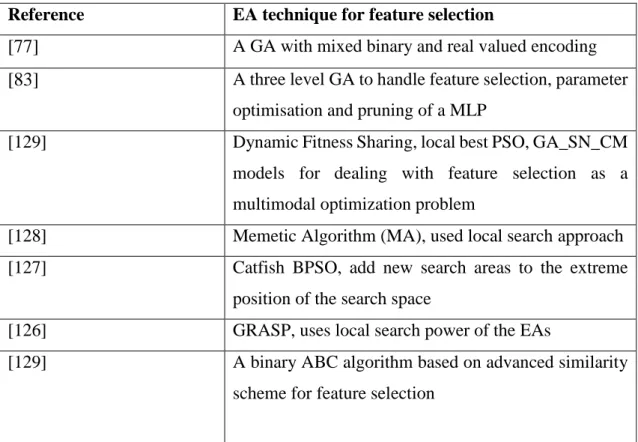
23 2.5 Evolutionary Feature selection

Several studies have investigated the effectiveness of EAs in feature selection. The aim of feature selection in classification problems is to obtain some representations of the dataset that are more adequate for learning the decision boundaries from that data samples [97]. Generally feature selection includes two objectives, namely maximizing classification accuracy and minimizing the number of features. both are often conflicting objectives. Therefore, feature selection can be considered as a multi-objective problem. On the other hand EAs that use population based approaches are effective in handling multi objective optimization problems [98]. Various studies adopted different kinds of EAs such as Genetic Algorithm (GA) [99-101] , PSO Algorithm [102-104] , Differential Evolution (DE) Algorithm [105] , Ant Colony Optimization (ACO) algorithm [106]. According to [107], PSO and GA are the most common EAs used for feature selection in classification problems. The feature selection approaches also would act as filter, wrapper, hybrid or embedded depending on the way they evaluate fitness of their population [98]. In wrapper methods, a classification algorithm is used to evaluate the subset of features [107]. Different classification algorithms were used in wrapper methods, e.g., SVMs [108-110]; KNN [111-113]; ANNs [114-116]; Decision Tree (DT) [117]; Naïve Bayes (NB) [117, 118]. In filter-base methods , different measures from various disciplines are adopted for feature selection, e.g., information theory-based measures [119], consistency measures [120], correlation measures [113] and distance measures[121] .

For GA based feature selection methods several enhancements to GAs are available, which focus mainly on the search mechanisms, representation, and the fitness function. Some early studies on GAs for feature selection are presented in [122] and [123]. Those studies investigated the influence of the population size, mutation, crossover, and reproduction operators, but with limited experiments. In [124] a bio-encoding scheme in a GA was proposed, where each chromosome included a pair of strings. The first string was binary-encoded to indicate the selection of features, and the second was encoded as real-numbers to represent the weights of the selected features. By combining the proposed method with an Adaboost learning algorithm, the bio-encoding scheme obtained better performance than binary encoding. In [125] a new representation was proposed that included both feature selection and parameter optimization of a classification algorithm, e.g., an SVM. The length was the total number of features and parameters. [115] developed a three-level representation of a GA and MLP for feature selection, which indicated the selection of features, pruning of the neurons, and the MLP architecture, respectively. These studies in [124], [125], and [115] indicated that

(39)

24

combining feature selection and optimization of a classification algorithm was an effective way to improve classification performance since both the data and the classifier are optimized. Several studies also proposed improvements of the exploration and local search powers of EAs for feature selection. These capabilities are crucial to better handle feature selection problems. As an example the GRASP model proposed in [126] involved an iterative process where each iteration compromised two phases of construction and local search. In the construction phase a potential solution was created, while its neighborhood was searched in search phase. The final solution was the best one found after all iterations. In [127] a new modification to the PSO algorithm called Catfish BPSO was proposed for feature selection. In Catfish BPSO a competition function was introduced to the individuals by defining the Catfish effect. If the fitness could not be improved over a number of iterations, the catfish particles were introduced. They initialized new search and opened up new opportunities for finding better solutions at extreme positions of the search space and guided the whole swarm to promising regions of the search space. Introducing catfish particles in Catfish BPSO algorithm helped avoid converging toward a local optimum solution by increasing the exploration power and diversity of its population.

In [128] Memetic Algorithm (MA), which consisted of a population based method and a local search mechanism to improve the solutions, was used for feature selection. MA utilised the advantages of local search as well as exploration of the search space to find effective and accurate feature subsets. In [98] a multi-modal optimization method was used for feature selection. It considered that the optimal subset of features might not be unique for the problem. Dynamic Fitness Sharing (DFS), local best PSO variants and GA_SN_CM, were proposed for feature selection with several benchmark data sets. The obtained results were compared with those from some well-known heuristic methods for feature selection using statistical analysis methods. The comparison results indicated the effectiveness of the proposed method.

In [129] a binary ABC algorithm was proposed for feature selection and its performance was statistically compared with common EA- based feature selection techniques with 10 benchmark problems. The proposed algorithm could converge more quickly, with less computational expenses.

(40)

25

In the following the GA is described in detail, as it is used for secondary features selection as well as optimization of the network parameters (weights) in the FLNN-based models in this research. Table 2.4 summarizes the EA based optimization techniques of the reviewed literature.

Table 2.4 Summary of papers on Evolutionary feature selectionation Reference EA technique for feature selection

[77] A GA with mixed binary and real valued encoding

[83] A three level GA to handle feature selection, parameter optimisation and pruning of a MLP

[129] Dynamic Fitness Sharing, local best PSO, GA_SN_CM

models for dealing with feature selection as a multimodal optimization problem

[128] Memetic Algorithm (MA), used local search approach [127] Catfish BPSO, add new search areas to the extreme

position of the search space

[126] GRASP, uses local search power of the EAs

[129] A binary ABC algorithm based on advanced similarity scheme for feature selection

Genetic Algorithm: The GA is a well-established EA invented by John Holland at University of Michigan. The design of GA, like ANNs, was inspired by the processes occurring in nature. The GA has been theoretically and empirically shown to perform consistently in complex search spaces [93]. The rationales behind the GA come from natural genetic processes. It involves terms such as gene, chromosomes, offspring, generation, crossover, and mutation. The GA begins with generating a random population of chromosomes (individuals) as the initial solution. A fitness or evaluation function, which reflects the problem objectives, is defined to determine the fitness of individuals in the population. During the process, the GA selects some chromosomes according to a particular criterion on the fitness value, and dismisses other chromosomes.

(41)

26

The GA progresses by developing offspring using reproduction processes. They are known as crossover and mutation that recombine and develop a new generation. As a result, a number of generations are iterated until the GA converges to the best solution, or stops when a given stopping criterion is reached. The main GA characteristics can be described as follows [93].

 Since the GA performs a stochastic search and does not require gradient information, it is an effective way for finding the global optimum solution of most problems, whether the corresponding function is differentiable or not.

 The GA is a multi-point search method. In other words, it considers multiple points in the search space simultaneously. As a result, the chance of finding the global optimum solution increases, and the probability of being trapped in local optima decreases.

 The GA is a robust method in the sense that it does not require information about the structure or parameters of the problem [117]. Therefore, it can be applied to almost all types of ANNs.

The pseudo-code for the GA is presented in Figure 2-6.

Figure 2-6: Pseudo code for standard GA algorithm 1: begin

2: Initialize population of individuals 3: Evaluate the fitness of each individual 4: while (not termination criterion) do:

5: Select the best individuals and send them to GA operators 6: Evaluate the fitness of new individuals from GA operators 7: Replace the least fit individuals by the best new individuals 8: end while