Time Series Data Mining Methods: A Review
Master’s Thesis submittedto
Prof. Dr. Wolfgang Karl H¨ardle Humboldt-Universit¨at zu Berlin School of Business and Economics Ladislaus von Bortkiewicz Chair of Statistics
by
Caroline Kleist (533039)
In partial fulfillment of the requirements for the degree of
Master of Science in Statistics Berlin, March 25, 2015
Abstract
Today, real world time series data sets can take a size up to a trillion observations and even more. Data miners’ task is it to detect new information that is hidden in this massive amount of data. While well known techniques for data mining in cross sections have been developed, time series data mining methods are not as sophisticated and established yet. Large time series bring along problems like very high dimensionality and up to today, researchers haven’t agreed on best practices in this regard.
This review gives an overview of the challenges of large time series and the proposed problem solving approaches from time series data mining community. We illustrate the most impor-tant techniques with Google trends data. Moreover, we review current research directions and point out open research questions.
Heutzutage sind die M¨oglichkeiten der Datensammlung und -Speicherung unvorstellbar weitreichend und somit k¨onnen Zeitreihendatens¨atze mittlerweile bis zu einer Billion Be-obachtungen enthalten. Die Aufgabe von Data Mining ist es, versteckte Informationen aus dieser Datenschwemme herauszufiltern. W¨ahrend es f¨ur Querschnittsdaten viele verschiedene und sehr gut entwickelte Techniken gibt, hinken die Zeitreihen Data Mining Methoden weit hinterher. Die Forschungspraxis hat sich in diesem Bereich noch nicht auf standardisierte Vorgehensweisen geeinigt.
Dieser Literatur¨uberblick stellt zun¨achst die typischen Probleme, die Zeitreihen mit sich bringen, dar und systematisiert daraufhin die von der Forschungsgemeinde vorgeschlagenen L¨osungsans¨atze hierf¨ur. Die wichtigsten Ans¨atze werden anhand von Google Trends Daten illustriert. Dar¨uber hinaus werfen wir einen Blick auf aktuelle Forschungsstr¨ome und zeigen noch offene Forschungsfragen auf.
Contents
List of Abbreviations iii
List of Figures v
List of Tables v
1 Introduction 1
2 Properties and Challenges of Large Time Series 2
2.1 Streaming Data . . . 3 3 Preprocessing Methods 4 3.1 Representation . . . 4 3.2 Indexing . . . 11 3.3 Segmentation . . . 12 3.4 Visualization . . . 14 3.5 Similarity Measures . . . 15
4 Mining in Time Series 23 4.1 Clustering . . . 23
4.2 Knowledge Discovery: Pattern Mining . . . 25
4.3 Classification . . . 28 4.4 Rule Discovery . . . 30 4.5 Prediction . . . 32 5 Recent Research 33 6 A Thousand Applications 35 7 Conclusion 37 References 38
List of Abbreviations
ACF Autocorrelation Function AIC Akaike Information Criterion
APCA Adaptive Piecewise Constant Approximation AR(I)MA Autoregressive (Integrated) Moving Average
CDM Compression Based Dissimilarity Measure DFT Discrete Fourier Transform
DTW Dynamic Time Warping
DWT Discrete Wavelet Transform
ECG Electro Cardiogram
ED Euclidean Distance
EDR Edit Distance on Real Sequence ERP Edit Distance with Real Penalty
fMRI Functional Magnetic Resonance Imaging ForeCA Forecastable Component Analysis
FTW Fast Dynamic Time Warping
GIR Global Iterative Replacement
HMM Hidden Markov Model
ICA Independent Component Analysis
iSAX Indexable Symbolic Aggregate Approximation
LCSS Longest Common Subsequence
LDA Linear Discriminant Analysis
MCMC Markov Chain Monte Carlo
MDL Minimum Description Length
MVQ Multiresolution Vector Quantized
NN Nearest Neighbor
OGLE Optical Gravitational Lensing Experiment PAA Piecewise Aggregate Approximation PACF Partial Autocorrelation Function
PCA Principal Component Analysis PFA Predictable Feature Analysis
PIP Perceptually Important Points PLR Piecewise Linear Representation
QbH Query by Humming
SARIMA Seasonal Autoregressive Integrated Moving Average SAX Symbolic Aggregation Approximation
SDL Shape Definition Query
SOM Self Organizing Maps
SpADe Spatial Assembling Distance
SPIRIT Streaming Pattern Discovery in Multiple Time Series SVD Singular Value Decomposition
SVDD Singular Value Decomposition with Deltas
SVI Search Volume Index
SVM Support Vector Machines
SVR Support Vector Regression
SWAB Sliding Window And Bottom Up
TB Terabyte
TQuEST Threshold Query Execution
TSDM Time Series Data Mining
List of Figures
1 PAA Dimension Reduction of Google Search Volume Index . . . 7
2 PAA and SAX Representation of Google Search Volume Indices . . . 9
3 Systematizations of Time Series Similarity Measures . . . 16
4 Dynamic Time Warping vs. Euclidean Distance . . . 17
5 DTW Cost Matrix . . . 19
6 Hierarchical Clustering Based on Euclidean Distances . . . 24
7 Similar Google SVIs According to Hierarchical Clustering . . . 26
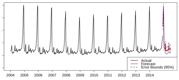
8 Prediction of Google Search Volume Index . . . 32
List of Tables
1 Tabulated SAX Breakpoints for Cutoff Lines . . . 101
Introduction
The buzzwordsdata mining andbig data are of strongly growing importance and found their way into mass media a few years ago. Moreover, big data is according to Forbes magazine (IBM, 2014) even labeled as the new natural resource of the century. Considering the various sources of big data in real life, this trend is not surprising. With the vast amount and variety of data available, the capacity of manual data analysis has been exceeded longly. So, the explosion of information available brings about not only ample opportunities but raises new challenges on data analysis methods. Therefore, data mining as a set of techniques for the analysis of massive datasets is of ever increasing importance as well.
In spite of these developments, it might sound surprising thattime series data mining is far behind cross sectional data mining techniques. While cross section techniques have been well developed, the time series data mining methods are not that sophisticated yet.
Generally speaking, data mining is the analytic process of knowledge discovery in large and complex data sets. It is a discipline at the very intersection of statistics and computer science as the search for hidden information is partly made automatic by employing computers for this task. To be more precise, data mining is the result of the hybridization of statistics, computer science, artificial intelligence and machine learning (Fayyad et al., 1996). Com-pared to times before computers and sensors were able to collect and store such bulky data sets, the paradigm of the methods of statistical operations has changed and partly gone into reverse. Today, a data scientist wants to find the needle in the hay and operates top down. In data mining, no a priori intended model is calibrated using known data. Mainly, data miners search for hidden information in the data like frequently recurring patterns, anoma-lies or natural groupings. Generally speaking, typical data mining tasks include knowledge discovery, clustering, classification, rule discovery, summarization and visualization.
In this paper, we review time series data mining methods. We present an overview of state of the art time series data mining techniques which become gradually established in the data mining community. Moreover, we point out recent and still open research areas in time series data mining. The search for real world applications and data sources yields numerous exam-ples. One well known data giant is Google. They processes on average over 40,000 search queries per second and store over 1.2 trillion search queries per year (Internetlivestats.com, 2014). We illustrate the most popular time series data mining techniques with Google trends data (Google, 2014).
The remainder of this paper is organized as follows. Section 2 shows characteristic prop-erties and thereof resulting challenges and problems of large time series. Section 3 discusses crucial preprocessing methods for time series including representation and indexing tech-niques, segmentation, visualization and similarity measures. Hereafter, Section 4 proceeds with typical data mining tasks tailored to time series: clustering, knowledge discovery, clas-sification, data streams, rule discovery and prediction. Section 5 points out recent research directions and Section 6 highlights the broad range of applications for time series data mining. Section 7 concludes.
2
Properties and Challenges of Large Time Series
Before we come up with time series data mining methods, we itemize which problems need to be tackled. As a general rule, large time series come along with super-high dimensional-ity, noise along characteristic patterns, outliers and dynamism. Moreover, the most crucial challenge in time series data mining is the comparison of two or more time series which are shifted or scaled through time or in amplitude.
The problems that need to be tackled in time series data mining arise from typical proper-ties of large time series. Firstly, as one observation of a time series is viewed as one dimension, the dimensionality of large time series is typically very high (Rakthanmanon et al., 2012). The visualization alone of time series which are larger than a several ten thousand observa-tions can be challenging Lin et al. (2005). Working with super-high dimensional raw data can be very costly with respect to processing and storage costs (Fu, 2011). Therefore, a high level representation of the data or abstraction is required. Besides, the basic philosophy of data mining implies that avoiding a potential information loss by studying the raw data is not convenient and too slow. In the context of time series data mining, noise along characteristic patterns are additive white noise components (Esling and Agon, 2012). Provided that we are interested in global characteristics, the time series data mining techniques need to be robust against noisy components. If such massive amounts of data are collected, the sensitivity to-wards measurement errors and outliers can be high. At the same time, long time series enable us to better differentiate between outliers and rare outcomes. Rare outcomes which would be categorized as outliers in small subsamples help us to better understand heterogeneity (Fan et al., 2014).
Moreover, time series data mining aims at the comparison of two or more time series or subsequences. However, time series are frequently not aligned in the time axis (Berndt and
Clifford, 1994) or the amplitude (Esling and Agon, 2012). Besides temporal and amplitude shifting differences, time series can have scaling or acceleration differences while still having very similar characteristics. Time series data mining methods need to be robust against these transformations and combinations of them.
Furthermore, we up front clarify what “large” means in the context of large time series. The manageable dimensions can reach up to 1 trillion = 1.000,000,000,000 time series ob-jects. For settlement, 1 trillion time series objects need roughly 7.2 terabyte storage space. Rakthanmanon et al. (2012) include a brief discussion ofa trillion time series object. They illustrate that a time series with one trillion observations would correspond to each and every heartbeat of a 123 year old human being.
Another compelling reason for the application of time series data mining methods is the emergence of such a massive amount of data that is too big to store. The incoming time series data is growing faster than our ability to process and store the raw data. Hence, the data has to be reduced immediately in order to achieve reasonable storage size of the data. A typical example for data that is too big to store is streaming data, or data streams. Data streams are continuously and at very fluctuating rates generated observations (Gaber et al., 2005). For instance, computer network traffic data or physical network sensors deliver such non stopping streams of information.
2.1 Streaming Data
Besides the already discussed properties of large time series data sets, continuousstream data
brings along further challenges. Streaming data is characterized by a tremendous volume of temporally ordered observations arriving at a steady high-speed rate, it is fast changing, and potentially infinite (Gaber et al., 2005). In some cases, the entire original data stream is even too big to be stored. Typically, data mining methods require multiple scans through the data at hand. But, constantly flowing data requires single-scan and online multidimensional analysis methods for pattern and knowledge discovery. Resulting from that, the use of data reduction and indexing methods is not only necessary but inevitable. Initial research on streaming data is primarily concerned with data stream management systems and Golab and ¨Ozsu (2003) provide a review in this regard. As technological boundaries are constantly pushed outwards and even more massive and complex data sets are collected day by day, the need for data mining techniques for potentially infinite volumes of streaming data is becoming more urgent. The trade-off between storage size and accuracy is for streaming data
methods even more important than for time series data mining in general. As the discussion of streaming data reaches far beyond the scope of this review, please refer to the survey by Gaber et al. (2005). Streaming data techniques are still in the early stages of development and they have a high relevance in real world applications. Therefore, this research area is labeled as the next hottest topic in time series data mining.
3
Preprocessing Methods
Before jumping into actual data mining, it is essential to preprocess the data at hand. Firstly, large time series data is often very bulky. Thus, directly dealing with such data in its raw format is expensive with respect to processing and storage costs. Secondly, we are dealing with time series which are no more comprehensible with the unaided eye in its raw format. Therefore we beforehand reduce dimensionality or segment the time series and then index them. In the light of lacking natural clarity of the raw data, visualization techniques and tools for large time series emerged and are presented here. Moreover, similarity measures are the backbone of all data mining applications and need to be discussed.
3.1 Representation
As already discussed in Section 2, large time series are super-high dimensional. Each obser-vation of a time series is viewed as one dimension. So, in order to achieve effectiveness and efficiency in managing time series, representation techniques that reduce dimensionality of time series are crucial and still a basic problem in time series data mining. If we reduce the dimension of a time series X of original length n to k n, we can reduce computational complexity fromO(n) toO(k). At the same time, we do not want to lose too much informa-tion and aim to preserve fundamental characteristics of the data. Furthermore, we require an intuitive interpretation and visualization of the reduced data set. So, desired properties of representation approaches are dimensionality reduction, a short computing time, preserva-tion of local and global shape characteristics and insensitivity towards noise (additive white noise components). The time series data mining community developed many different rep-resentation and indexing techniques that aim to satisfy these requirements. The approaches differ with respect to their ability to address these properties. According to the various available representation techniques, a large number of different systematizations of represen-tation approaches exists. One common approach is to seperate represenrepresen-tation techniques corresponding to their domain and indexing form. Many approaches transform the original
data to another domain for dimensionality reduction and then apply an indexing mechanism. But, a more practically orientated systematization of representation techniques is proposed by Ding et al. (2008): For practical purposes, it is important to know whether the represen-tation techniques at hand aredata adaptive,non data adaptive or model based.
3.1.1 Non Data Adaptive Representation Techniques
Non data adaptive representation techniques are stiff and have always the same transfor-mation parameters regardless the features of the data at hand. So, the transfortransfor-mation pa-rameters are fixed a priori. One subgroup of non data adaptive representation techniques are operating in the frequency domain. Their logic follows the basic idea of spectral decom-position: any time series can be represented by a finite number of trigonometric functions. Generally speaking, operating in the frequency domain is valid as the Euclidean distances between two time series is the same in the time domain and in the frequency domain and hereby preserve distances. For example,DiscreteFourierTransform (DFT) as proposed by Agrawal et al. (1993a) for mining sequence databases preserves the essential characteristics of time series in the first few Fourier coefficients which are single complex numbers representing a finite number of sine and cosine waves. Only the first “strongest” coefficients of the DFT are kept for lower bounding of the actual distances.
Among others, Graps (1995), Burrus et al. (1998) and Chan and Fu (1999) point out that
Discrete Wavelet Transform (DWT) is an effective replacement for DFT. Opposed to the DFT representation, in DWT we consider not only the first few global shape coefficients, but we use both, coefficients representing the global shape as well as “zoom in” coefficients representing smaller, local subsections. The DWT consists of wavelets (which are functions) representing the data and is calculated by computing the differences and sum of a benchmark “mother” wavelet. Popivanov and Miller (2002) demonstrate that a large class of wavelets are applicable for time series dimension reduction. A major drawback of using wavelets is the necessity to have data with its length being an integer power of two. One popular wavelet is the so called “Haar” wavelet proposed to use in the time series data mining context by Struzik and Siebes (1999).
Other, more recently proposed non data adaptive representation techniques are especially tailored to time series data mining. The most popular approach from this group was in-troduced by Keogh and Pazzani (2000b) and is called Piecewise Aggregate Approximation
(PAA) since the research by Keogh et al. (2001a). Originally, Keogh and Pazzani (2000b) called the PAA methodPiecewiseConstantApproximation (PCA) and the name was after-wards changed to PAA as the abbreviationPCAis already reserved for Principal Component Analysis. The PAA coefficients are generated by dividing the time series into ω equi-sized windows and calculating averages of the subsequences in the corresponding windows. The averages of each window are stacked into a vector and called “PAA coefficients”. Hence, the dimension reduction of a time seriesX of lengthn into a stringXb = ˆx1, . . . ,xˆω of arbitrary
lengthω with ωnis performed by the following transformation:
ˆ xi =d−1 d i X j=d(i−1)+1 xj, i= 1, . . . , ω, j= 1, . . . , n, d=n w−1 (1)
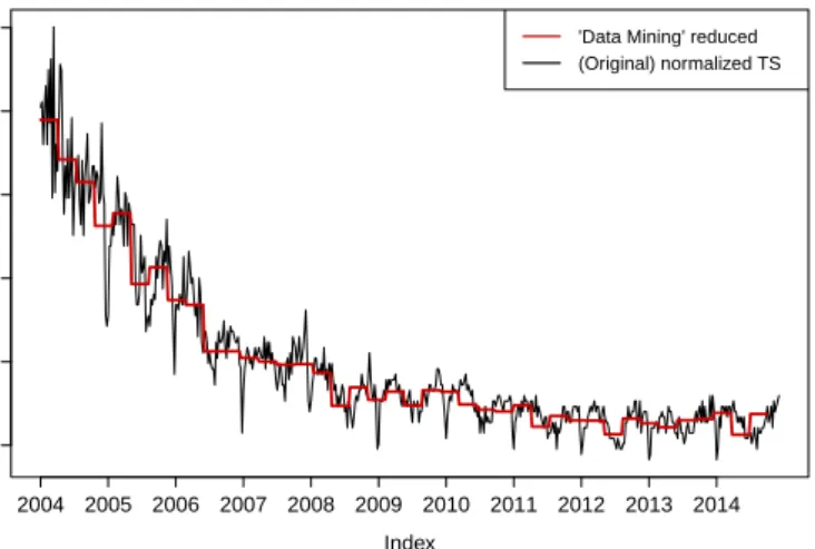
Figure 1 shows the PAA dimension reduction of the Google search volume index for the query term “Data Mining” withω= 40. Although the PAA dimension reduction approach is very simple, it is well comparable to more complex competitors (see for example Ding et al. (2008)). Furthermore, a very strong advantage is the fact that each PAA window is of the same length. This facilitates the indexing technique enormously (see Subsection 3.2). An extension of the PAA approach isAdaptivePiecewiseConstant Approximation (APCA) by Keogh et al. (2001b). APCA aims to approximate a time series by PAA segments of varying length, i.e. it allows the different windows to have an arbitrary size. In this way, we try to minimize the individual reconstruction error of the reduced time series. For the APCA, we do not only store the mean for each window but its length as well.
PrincipalComponentAnalysis (PCA) is a further dimension reduction technique adopted from static data approaches (see for instance Yang and Shahabi (2005b) or Raychaudhuri et al. (2000)). PCA disregards less significant components and therefore gives a reduced represen-tation of the data. PCA compurepresen-tations are based on orthogonal transformations with the goal to obtain linearly uncorrelated variables, the so called principal components. So, in order to reduce dimensionality, PCA requires the covariance matrix of the corresponding time series. However, for the covariance calculations it is ignored whether the considered time series are similar or correlated at different points in time. If two time series are evolving very similar and are only shifted in time, the traditional PCA approach would lead to false conclusions. To avoid this ineffectiveness, Li (2014) present an asynchronism-based principal component analysis. In order to improve PCA, Li (2014) embed Dynamic Time Warping (DTW, see Section 3.5.1) before applying PCA. By doing that, they employ asynchronous and not only synchronous covariances. Furthermore, DTW does not require the time series to be of the
−1 0 1 2 3 4
PAA reduction of SVI for 'Data Mining'
Index
SVI f
or 'Data Mining'
2004 2005 2006 2007 2008 2009 2010 2011 2012 2013 2014 'Data Mining' reduced (Original) normalized TS
Figure 1: PAA dimension reduction of the Google search volume index (SVI) for the query term “Data Mining” withn= 569 and ω = 40. Averages are calculated for all observations
falling into one window. TSDMPaa
same length as PCA does.
Opposed to all representation methods presented so far, Ratanamahatana et al. (2005) and Bagnall et al. (2006) hold the view that we do not have to compress the raw data by aggrega-tion of dimensions. Instead, they store a proxy replacing each real valued time series object. Namely, Ratanamahatana et al. (2005) and Bagnall et al. (2006) propose to store bits instead of all real valued time series objects and therefore obtain a so called clipped representation of the time series which needs less storage space and still has the same length n.
3.1.2 Data Adaptive Representation Techniques
Data adaptive representation techniques are (more) sensitive to the nature of the data at hand. The transformation parameters are chosen depending on the available data and not fixed a priori as for non data adaptive techniques. However, almost all non data adaptive techniques can be turned into data adaptive approaches by adding data-sensitive proceeding schemes.
TheSingularValueDecomposition (SVD) which is also known as Latent Semantic Indexing is said to be an optimal transform with respect to reconstruction error (see for example Ye (2005)). For SVD construction, we linearly combine the basis shapes best representing the original data. This is done by a global transformation of the whole dataset in order to maximize the variance carried by the axes. Finally, if we try to reconstruct the original data
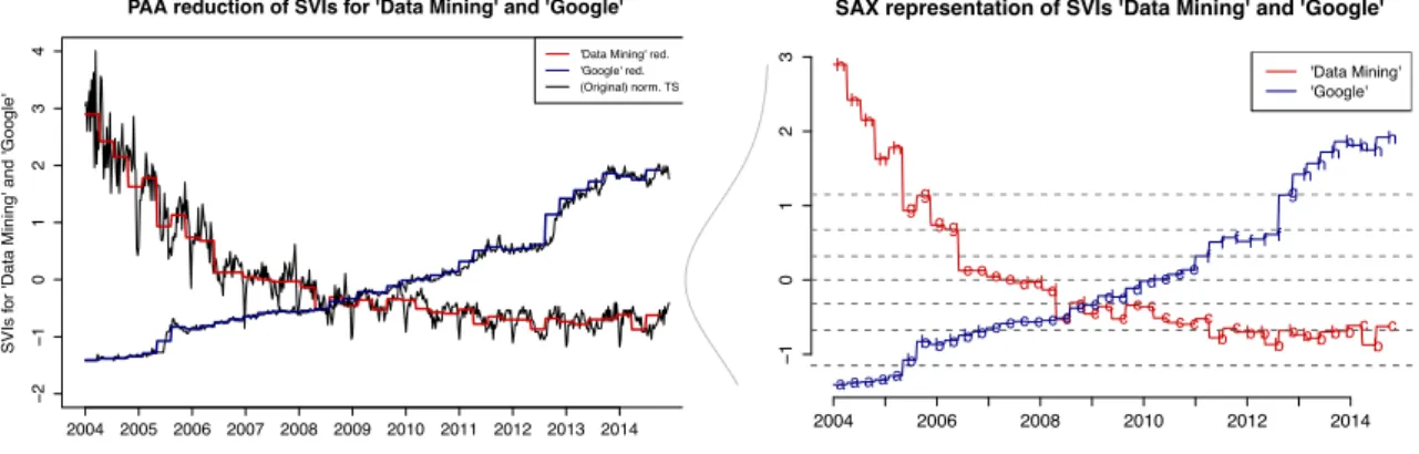
from the SVD representation, the error we make is relatively low. Korn et al. (1997) even aim to further minimize the reconstruction error and further improve the SVD representation. For this purpose they introduceSingularValue Decomposition withDeltas (SVDD). A very frequently used and probably the most popular dimensional reduction and indexing technique is based on a symbolic representation and called SAX. It was introduced by Lin et al. (2003). TheSymbolicAggregate Approximation (SAX) represenation is said to outperform all other dimensionality reduction techniques (see for instance Ratanamahatana et al. (2010) or Kadam and Thakore (2012)). In order to illustrate how the SAX algorithm works, Figure 2 shows the SAX representation including the PAA representation which is the preceding interim dimension reducing stage of the SAX algorithm. The illustrating example is computed for the trajectories of the Google SVI for the query terms “Data Mining” and “Google”. As already indicated, the transformation of a time series X of length n into a string X = x1, . . . , xω of arbitrary length ω with ω n is performed in two steps. In a first step, the
z-normalized time series is converted to a PAA representation, i.e. the Piecewise Aggregate
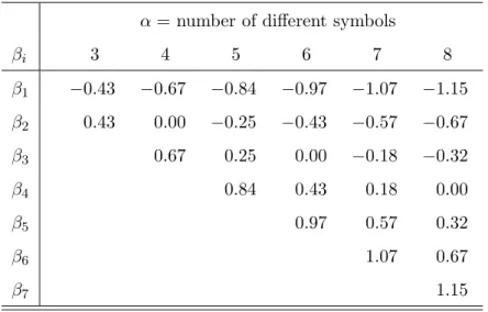
Approximation. As a reminder, the PAA coefficients are derived by slicing the data at hand along the temporal axis intoωequidistant windows and thereupon calculating sample means for all observations falling into one window (see Equation 1). Hereafter, the PAA coefficients are mapped to symbols (mostly letters). For doing so, the cutoff lines dividing the distribution space into α equiprobable segments need to be specified. Assuming that the z-normalized time series are standard normally distributed, these cutoff lines are tabulated forα different symbols as reported in Table 1. Hence,αis a hyperparameter that has to be chosen a priori. Equation 2 depicts how the PAA coefficients from the vector Xb = ˆx1, . . . ,xˆω are mapped
intoα different symbols yielding the SAX stringX =x1, . . . , xω:
xω=αj if xˆi ∈[βj−1, βj) (2)
with β1, . . . , βi being the corresponding tabulated breakpoints as reported in Table 1 for
i, j= 1, . . . , α−1. Finally, as symbols require fewer bits than real valued numbers, symbols are stored instead of the original time series. If we chose the hyperparameter to be α = 3, the three used symbols are “a”, “b” and “c”. Instead of the PAA coefficients or even the real valued time series objects, the symbols are stored in the corresponding order as a “word”. In order to speed the SAX algorithm dramatically up, Shieh and Keogh (2008) propose a modification of the SAX representation calledindexableSymbolicAggregateApproximation (iSAX). This multi-resolution symbolic representation allows extensible hashing and hence
− 2 − 1 0 1 2 3 4
PAA reduction of SVIs for 'Data Mining' and 'Google'
Index
SVIs f
or 'Data Mining' and 'Google'
2004 2005 2006 2007 2008 2009 2010 2011 2012 2013 2014
'Data Mining' red. 'Google' red. (Original) norm. TS − 1 0 1 2 3
SAX representation of SVIs 'Data Mining' and 'Google'
2004 2006 2008 2010 2012 2014 h h h hh gg g g e e e ed d d cdc c cc cc c c c bc b bbb b b b bcbc a a a a a bb b b b b cc c c c c c cd d d d e ee ff f f f f gh hhh h h h 'Data Mining' 'Google'
Figure 2: PAA dimension reduction (left) of Google search volume indices (SVIs) for the query terms “Data Mining” and “Google” with n = 569 and ω = 40 respectively. Corre-sponding SAX representation (right) withω= 40 andα= 8. In case of the SVI for the query term “Google”, the raw data is replaced by the word
“aaaaabbbbbbccccccccddddeeeffffffgh-hhhhhh”. TSDMSax
indexing of terabyte sized time series. Extensible hashing is a database management system technique (see for example Fagin et al. (1979)).
If we want to automatize the decision on the quantity of the hyperparameterα, we can use the
MinimumDescriptionLength (MDL) algorithm by Rissanen (1978). MDL is a computational learning concept and extracts regularities which lead to the best compressed representation of the data. In our context, MDL chooses that SAX representation depending on α which suffices and optimizes the trade-off between goodness-of-fit and model complexity.
Moreover, other symbolic representations than SAX exist. Megalooikonomou et al. (2005) propose the Multiresolution Vector Quantized (MVQ) approximation which is a multireso-lution symbolic representation of time series. M¨orchen and Ultsch (2005) develop a symbolic representation through an unsupervised discretization process incorporating temporal infor-mation. Li et al. (2000) arrive at a symbolic representation using fuzzy neural networks for clustering prediscretized sequences. The prediscretizing step is performed using a piecewise linear segmentation representation first.
Ye and Keogh (2009) propose a new representation approach called Shapelets. Shapelets are capturing the shape of small time series subsequences. Ye and Keogh (2009) propose Shapelets especially for classification tasks. Aside from that, Zhao and Zhang (2006) take recent-biased time series into account. They embed traditional dimension reduction tech-niques into their framework for recent-biased approximations.
α= number of different symbols βi 3 4 5 6 7 8 β1 −0.43 −0.67 −0.84 −0.97 −1.07 −1.15 β2 0.43 0.00 −0.25 −0.43 −0.57 −0.67 β3 0.67 0.25 0.00 −0.18 −0.32 β4 0.84 0.43 0.18 0.00 β5 0.97 0.57 0.32 β6 1.07 0.67 β7 1.15
Table 1: Tabulated SAX breakpoints for the corresponding cutoff lines for 3 to 8 different symbols as reported in Lin et al. (2003). Corresponding to the hyperparameterα, the break-point parameters are chosen data independently. The breakbreak-points are determined based on the assumption that thez-normalized time series are standard normally distributed.
Lastly, Wen et al. (2014) recently proposed an adaptive sparse representation for massive spatial-temporal remote sensing.
3.1.3 Model Based Representation Techniques
The paradigm of model based representation techniques builds on the idea that the data at hand has been produced by an underlying model. Therefore, these techniques try to find the parametric form of the corresponding underlying model. One simple approach is to represent subsequences with best fitting linear regression lines (see for example Shatkay and Zdonik (1996)). Or we can employ more complex and better suited models as the AutoRegressive
Moving Average (ARMA) model and moreover, we can adduce Hidden Markov Models (HMM, see for example Azzouzi and Nabney (1998)).
Unfortunately, there is no general answer to the question which representation technique
isthe best. The answer is: it depends. It depends on the data at hand and the purposes we are
pursuing with our analysis. For example, if we want to get an idea of overall shapes and trends, the more globally focused approaches like DFT suite well. Or, if we want to incorporate wavelets, we need to have data with its length being an integer power of two. Highly periodic data is most likely treated best by spectral methods. Generally, the paper by Keogh and
Kasetty (2003) and Wang et al. (2013) both show that the different representation methods are overall performing very similar in terms of speed and accuracy. They use the tightness of lower bounding as measure for comparison of the manifold representation techniques. Furthermore, we have to regard that the choice of the dimensionality reduction technique determines the choice of an indexing technique (see Section 3.2). PAA, DFT, DWT and SVD naturally lead to an indexable representation.
3.2 Indexing
Representation and indexing techniques for time series work hand in hand with each other. Time series indexing schemes are designed for efficient time series data organization and especially for a quick processing request in large databases. If we want to find the closest match to a given query time series X in a database, a sequential or linear scan of the whole database is very costly. The access to the raw data is inefficient as it can take quite a long time. Therefore, indexing schemes are required to be much faster than sequential or linear scanning of the time series database. Hence, we store two representation levels of the data: on the one hand the raw data and on the other a compressed high level representation version of the data (see Section 3.1 for the different representation techniques). Then, we perform a linear scan for our query on the compressed data and compute a lower bound to the original distances to the query time series X. To put it in simpler words, the indexing is used to retrieve a rough first result from the database at hand. This quick and dirty result is used for a further, more detailed search for certain (sub)sequences. So, we try to avoid scanning the whole database but only examine certain sequences further which come into question. Moreover, we build an index structure for an even more efficient similarity search in a database. We group similar indexed time series into clusters and access only the most promising clusters for further investigations. Index structure approaches can be classified into vector based and metric based index structures. Vector based index structures firstly re-duce the data’s dimensionality and then clusters the vector based compressed sequences into similar groups. The clustering technique can be hierarchical and non-hierarchical. R-Tree by Guttman (1984) is the most popular non-hierarchical vector based index structure. For in-dexing the first few DFT coefficients, Agrawal et al. (1993a) adopt the R*-tree by Beckmann et al. (1990). Faloutsos et al. (1994) focus on subsequence matching and employ R*-trees as well.
cluster the sequences with respect to relative distances to each other. Yang and Shahabi (2005a) propose a multilevel distance-based index structure for multivariate time series. Vla-chos et al. (2003a) index multivariate time series incorporating multiple similarity measures at the same time. The index by Vlachos et al. (2006) can accommodate multiple similarity measures and can be used for indexing multidimensional time series.
As mentioned above, the choice of the indexing structure can depend on the a priori made decision on the corresponding representation technique. In this context, we recite more repre-sentation specific indexing structures. Rafiei and Mendelzon (1997) build an similarity based index structure based on Fourier transformations. Agrawal et al. (1993a) build an index structure based on DFT coefficients and Kahveci and Singh (2004) focus on wavelets based index structures. Chen et al. (2007a) introduce indexing mechanisms for Piecewise Linear
Representation, (PLR, see Section 3.3) and Keogh et al. (2001d) introduce the ensemble-index which combines two or more time series representation techniques for more effective indexing.
Lastly, Aref et al. (2004) present an algorithm for partial periodic patterns in time series databases and address the problem of so called merge mining. In merge mining, discovered patterns of two or more databases that are mined independently are merged, see for example Aref et al. (2004).
3.3 Segmentation
Segmentation is a discretization problem and aims to accurately approximate time series. As representation techniques (see Section 3.1) strive for similar purposes, the boundaries between segmentation and shape representation techniques are blurred. Bajcsy et al. (1990) even make the point that both preprocessing steps should not be handled separately. Yet historically grown, still other discretization and dimension reduction techniques than those discussed in Section 3.1 are subsumed under the concept of segmentation.
Time series are characterized by their continuous nature. Segmentation approaches reduce the dimensionality of the time series while preserving essential features and characteristics of the original time series. The general approach is to firstly segment a time series into subsequences (windows) and to secondly choose primitive shape patterns which represent the original time series best. The most intuitive time series segmentation technique is called PLR, the Piecewise Linear Representation (see for example Zhu et al. (2007)). The idea is
to approximate a time series X of length n by k linear functions which are the segments then. But this segmentation technique highly depends on the choice of k and slices the time series in equidistant windows. This fixed-length segmentation comes along with obvious disadvantages. Therefore, we are interested in more flexible and data-responsive algorithms. Keogh and Pazzani (1998) introduce a PLR technique which uses weights as well accounting for the relative importance of each individual linear segment and Keogh and Pazzani (1999) add relevance feedback from the user.
Following Keogh et al. (2004a), the segmentation algorithms which result in a piecewise linear approximation can be categorized into three major groups of approaches: top down, bottom up and sliding windows approaches. Top down approaches recursively segment the raw data until some stopping criteria are met. Top down algorithms are used in many research areas and known under several names. The machine learning community for example knows it under the name “Iterative End-Points Fit” as named by Duda et al. (1973). Park et al. (1999) modify the top down algorithm by firstly scanning the whole time series for extreme points. These peaks and valleys are used as segmental starting points and then the top down approach refines the segmentation. Opposed to top down approaches, bottom up approaches start with the finest possible approximation and join segments until some stopping criteria are met. The finest possible approximation of an-length time series aren/2 segments. Both, the top down and bottom up approaches are offline and need to scan the whole data set. Therefore, they operate with a global view on the data. Sliding windows anchor the left point of a potential segment and try to approximate the data to the right with increasing longer segments. A segment increases until it exceeds some predefined error bound. The next time series object not included in the newly approximated segment is the new left anchor and the process repeats. Sliding windows algorithms are especially attractive as they are online algorithms. However, sliding window algorithms are according to Keogh et al. (2004a) and Shatkay and Zdonik (1996) producing poor segmentation results if the time series at hand contains abrupt level changes as they cannot look ahead. The bottom up and top down approaches which operate with a global view on the data produce better results than sliding windows (see e.g. Keogh et al. (2004a)). By combining the bottom up approach and sliding windows, Keogh et al. (2001c) try to offset the disadvantages of the respective technique mutually. They propose theSlidingWindow AndBottom Up (SWAB) segmentation algorithm which allows an online approach with “semi-global” view.
we can apply are manifold. All these techniques aim at the identification of in some way prominent points which are used for decisions in the three segmentation approaches. A common method is according to e.g. Jiang et al. (2007) or Fu et al. (2006) the Perceptually
ImportantPoints (PIP) method as introduced for time series by Chung et al. (2001). Besides that, a plethora of different techniques are proposed. Oliver and Forbes (1997) pursue a change point detection approach, Bao and Yang (2008) propose turning points sequences applied to financial trading strategies, Guralnik and Srivastava (1999) present a special event detection, Oliver et al. (1998) and Fitzgibbon et al. (2002) use minimum message length approaches, and Fancourt and Principe (1998) tailor PCA to locally stationary time series. Duncan and Bryant (1996) suggest to use dynamic programming for time series segmentation. Himberg et al. (2001) speed the dynamic programming approaches up by approximating them with Global Iterative Replacement (GIR) algorithm results and they illustrate their segmentation technique with mobile phone applications in context recognition. Wang and Willett (2004) use a piecewise generalized likelihood ratio for a rough, first segmentation and then elaborate the segments further. Fancoua and Principe (1996) perform a piecewise segmentation with an offline approach and furthermore map similar segments as neighbors in a neighborhood map. Recently, Cho and Fryzlewicz (2012) segment a piecewise stationary time series with unknown number of breakpoints using a nonparametric locally stationary wavelet model.
Moreover, the segmentation of multivariate time series is an active research area. Dobos and Abonyi (2012) combine recursive and dynamic Principal Component Analysis (PCA) for multivariate segmentation. Lastly, in a very recent paper by Guo et al. (2015), dynamic programming is applied in order to tackle multivariate time series segmentation automatically.
3.4 Visualization
Due to the massive size of the data, an actually simple task like visualization can very fast become anything but trivial. As a result of the very high dimensionality of large time se-ries, plotting a univariate time series using a usual line plot is unrewarding. Accordingly, the need for manageable and intuitive data visualization gives rise to several visualization tools. The most popular representatives of the recent visualization approaches or interfaces are Calendar-Based visualization, Spiral, TimeSearcher and VizTree.
Calender-Based visualization by Van Wijk and Van Selow (1999) is based on the idea of
The time series are chunked into daily sequences and clusters are computed for similar daily sequential patterns. Furthermore, a calendar with color-coded clusters is shown.
The Spiral by Weber et al. (2001) is mainly used for detecting periodic patterns and
struc-tures in the data. Periodic patterns are mapped onto rings and assigned to colors and the line width is corresponding to their features. But implicitly, the Spiral is only useful for data with periodic structures.
Time Searcher by Hochheiser and Shneiderman (2004) and Keogh et al. (2002a) requires a
priori knowledge about the data at hand as we need to have at least an idea of what we are searching for. We need to insert query orders which are called “TimeBoxes” for zooming in on certain patterns.
The most recent tool and most promising of these four is VizTree by Lin et al. (2005). The VizTree interface provides both, a global visual summary of the whole time series and the possibility to zoom in for interesting subsequences. So, VizTree is suited best for data min-ing tasks as we can discover hidden patterns without previous knowledge about the data. VizTree firstly computes a symbolic representation of the data and then builds a suffix tree. In the suffix tree, characteristic features of patterns and frequencies are mapped onto colors. VizTree is suited for the discovery of frequently appearing patterns as well as the detection of outliers and anomalies.
Moreover, Kumar et al. (2005) propose a user friendly visualization tool which employs simi-larities and differences of subsequences within a collection of bitmaps. Lastly, Li et al. (2012) introduce a motif visualization system based on grammar induction. For this visualization system, no a priori knowledge about motifs is required and the motif discovery can take place for time series with variable lengths.
3.5 Similarity Measures
Similarity measures indicate the level of (dis)similarity between time series. They are at the same time the backbone and the bottleneck of time series data mining. As similarity measures are needed for almost all data mining tasks (i.e. pattern discovery, clustering, clas-sification, rule discovery and novelty detection) they are the backbone of time series data mining. Coincidentally, similarity measures impose the major capacity constraints on time series data mining algorithms (Rakthanmanon et al., 2012). The faster the similarity measure computation algorithm, the faster is the whole time series data mining procedure as the main computing time is needed for the similarity measure calculations.
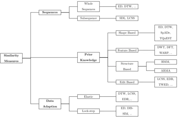
Similarity Measures Data Adaption Lock-step ED, DIS-SIM, .. Elastic DTW, LCSS, EDR,... Prior Knowledge Edit Based LCSS, EDR, TWED, ... Structure Based ARMA HMM, Feature Based DWT, DFT, WARP, .. Shape Based ED, DTW, SpADe, TQuEST Sequences Subsequence SDL, LCSS Whole Sequences ED, DTW, ...
Figure 3: Possible systematizations of time series similarity measures.
Similarity measures are required to be robust against scaling differences between time series, warping in time, noise along characteristic patterns and outliers (Esling and Agon, 2012). Scaling robustness includes robustness against amplitude modifications and warping robust-ness corresponds to robustrobust-ness against temporal modifications. A “noisy” time series is here interpreted as a time series with an additive white noise component.
Similarity measures are not only the capacity bottleneck of the time series data mining pro-cess with respect to time, but they govern the number of dimensions we can deal with, too. So, the processable dimensions of time series datasets depend on the manageable dimensions for the similarity search. Rakthanmanon et al. (2012) were the first to develop a similarity search algorithm based on dynamic time warping (see Section 3.5.1) that allows mining a
trillion time series objects. Up to that paper, time series data mining algorithms were
lim-ited to a few million observations (if one requires an acceptable computing time). But at the same time industry possesses massive amounts of time series waiting to be explored; speeding similarity search up in order to mine trillions of time series objects is a breakthrough in time series data mining.
Time series data mining community proposed a plethora of different similarity measures and distance computation algorithms. Also, many different systematizations of time series simi-larity measures exist (see Figure 3). We take over the systematization by Esling and Agon (2012) who classify similarity measures into four categories: shape based, edit based, feature
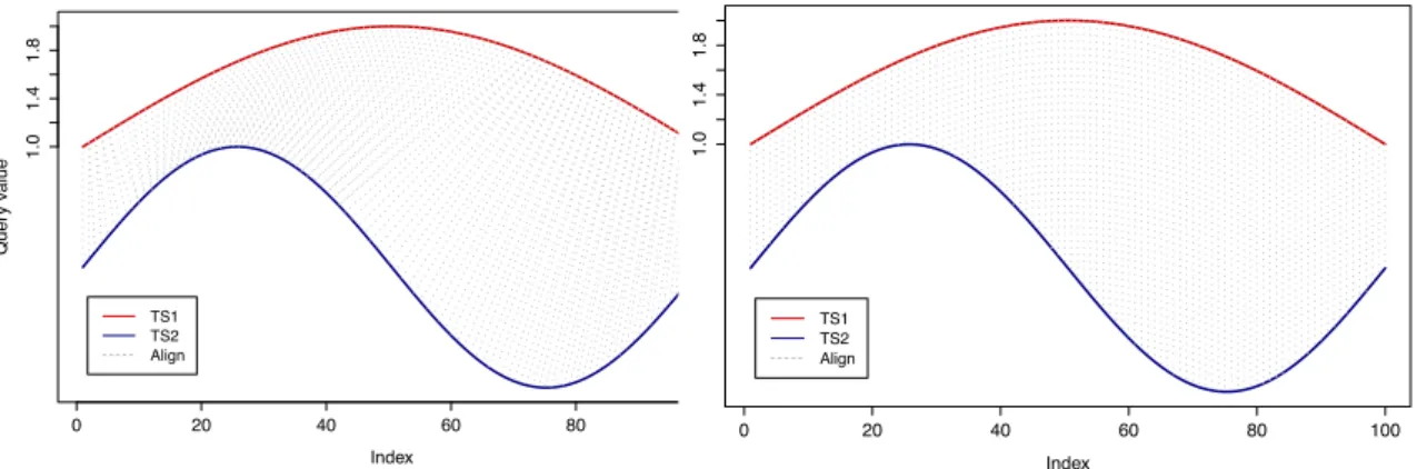
Index Quer y v alue 0 20 40 60 80 100 1.0 1.4 1.8 TS1 TS2 Align Index Quer y v alue 0 20 40 60 80 100 1.0 1.4 1.8 TS1 TS2 Align
Figure 4: Dynamic time warping (left) vs. Euclidean distance (right): DTW searches the optimal alignment path through the distance matrix consisting of all pairwise Euclidean distances between the two time series X and Y. TSDMDtw
based and structure based similarity measures. Furthermore, we distinguish between elastic and lock-step similarity measures. Lock-step measures compare the i-th point of time series X to the i-th point of time series Y. In contrast to that, elastic similarity measures allow a flexible comparison and additionally compare one-to-many or one-to-none points of X to Y. The also useful systematization of similarity measures into sequence and subsequence matching approaches is discussed in Fu (2011).
3.5.1 Shape Based Similarity Measures
Shape based similarity measures compare the global shape of time series. AllLp norms,
espe-cially the popular Euclidean distance, are widely used similarity measures (Yi and Faloutsos, 2000). Nevertheless, in time series similarity computations, Lp norms deliver poor results
(see for example Keogh and Kasetty (2003) or Ding et al. (2008)) as they are not robust against temporal or scale shifting. As they are lock-step measures, the length and position in time of the two time series which we want to compare need to be the same.
Opposed to that, the most popular elastic shape based similarity measure is Dynamic
TimeWarping (DTW) and especially proposed to handle warps in the temporal dimension. Temporal warping corresponds to shifting and further modifications in the temporal axis. DTW is said to be the most accurate similarity search measure (see for example Rakthan-manon et al. (2012), Ding et al. (2008)). After its introduction it was firstly popular in speech recognition (Sakoe and Chiba (1978)) and nowadays it is used in manifold domains,
for example for online signature recognition. Berndt and Clifford (1994) were the first to use DTW in data mining processes. Figure 4 shows a DTW alignment plot and for comparison Euclidean distances between two time series. DTW is proposed to overcome inconveniences of rigid distances and to handle warping and shifting in the temporal dimension, i.e. the two temporal sequences may vary in time or speed. Furthermore, DTW allows to compare time series of different length. Even an acceleration or deceleration during the course of events is manageable. In order to compute a DTW distance measure between two time se-ries X = {x1, x2, . . . , xN} and Y = {y1, y2, . . . , yM} with N, M ∈ N, two general steps are
necessary. Firstly, a cost (or “distance”) matrix D(N×M) as shown in Figure 5 has to be calculated. For this purpose, predefined distances (most often Euclidean distances) between
all components of X and Y have to be computed. Each entry of the cost matrix D(N×M) corresponds to the Euclidean distance between a pair of points (xi, yj). Secondly, we look
for the optimal alignment path betweenX and Y as a mapping between the two time series. The optimal alignment between two time series results in minimum overall costs, i.e. the minimum cumulative distance. The basic search for the optimal alignment path through the cost matrix is subject to three general conditions: (i) boundary, (ii) monotonicity and (iii) step size conditions. The boundary condition ensures that the first and the last observations of both time series are compared to each other. So, the start of the alignment path in the cost matrix is fixed as D(0,0) and the end as D(N, M). The monotonicity and step size conditions ensure that the alignment path moves always up or right or both at once but never backwards. Using dynamic programming, the computing time of DTW has complexity O(n2) (Ratanamahatana and Keogh, 2004).
Additionally, many extensions to the classical DTW exist. Further constraints (especially lower bounding measures) aim to speed up the matching process. Ding et al. (2008) rec-ommend to generally use constrained DTW measures instead of plain DTW. Constraining the warping window size can reduce computation costs and enable effective lower-bounding while resulting in the same or even better accuracy. The most frequently applied global con-straint is the Sakoe-Chiba band. Sakoe and Chiba (1978) place a symmetric band around the cost matrix’ main diagonal. The optimal alignment path is forced to stay inside this band. The Itakura parallelogram is a further very frequently used global path constraint. Itakura (1975) place a parallelogram around the cost matrix’ main diagonal constraining the warping range. A further common constraint is the lower bounding of the DTW distance. Lower bounding conditions require that the approximated DTW distance is at least as large
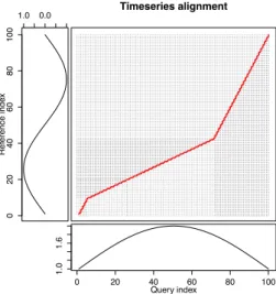
Timeseries alignment d$index1 d$inde x2 Query index xts 0 20 40 60 80 100 1.0 1.6 yts Ref erence inde x 1.0 0.0 0 20 40 60 80 100
Figure 5: Corresponding DTW cost matrix with the query index (reference index) corre-sponding to time series X (Y). The diagonal would represent the case for fixed Euclidean distances in the right panel of Figure 4. The red line is the optimal alignment path for time series X andY in the left panel of Figure 4. By minimizing overall costs, i.e. by minimizing the cumulative distance through the cost matrix, we find the optimal alignment path.
TSDMDtw
as the actual DTW distance. The most common lower bound condition is proposed by Keogh and Ratanamahatana (2005). They introduce the upper and lower envelope representing the maximum allowed warping which reduces computing complexity toO(n).
Moreover, modifications and extensions of DTW exist. Yi et al. (1998) use a FastMap tech-nique for an approximate indexing of DTW. Salvador and Chan (2007) introduce the ap-proximation of DTW, called FastDTW. This algorithm recursively projects a solution from a coarse solution to a higher resolution and then refines it. Fast DTW is on the one hand only approximative but on the other hand, it enables linear computing time. Chu et al. (2002) introduce an iterative deepening DTW approach and Sakurai et al. (2005) present theirFast DynamicTime Warping (FTW) similarity search. Fu et al. (2008) combine the locally flex-ible DTW with globally flexflex-ible uniform scaling which leads to search pruning and speeds up the search as well. Furthermore, Keogh and Pazzani (2000a) show that operating with the DTW algorithm on the higher level PAA representation instead of the raw data does not lead to a loss of accuracy.
Until 2012, the main disadvantage of DTW is said to be the computational complexity. DTW computation was too slow to be used for truly massive databases. But Rakthanmanon et al.
(2012) proposed a new DTW based exact subsequence search suite of four novel ideas they are calling theUCR suite. They normalize the time series subsequences, reorder abandoning, reverse the query/data role in lower bounding and cascade lower bounds. Rakthanmanon et al. (2012) hereby facilitate mining of time series with up to a trillion observations.
Besides DTW and its modifications, many other shape based similarity measures exist. Frent-zos et al. (2007) introduce the index based DISSIM metric and Chen et al. (2007b) introduce the shape based Spatial Assembling Distance (SpADe) algorithm which is able to handle shifting in the temporal and amplitude dimensions. Aßfalg et al. (2006) propose TQuEST, a similarity search based on threshold queries in time series databases which report those se-quences exceeding a query threshold at similar time frames as the query time series. Goldin and Kanellakis (1995) impose constraints on similarity queries formalizing the notion of exact and approximate similarity.
3.5.2 Edit Based Similarity Measures
The main idea of edit based similarity measures is to assemble the minimum number of op-erations needed to transform time series X into time seriesY.
Lin and Shim (1995) introduce a similarity concept that captures the intuitive notion that two sequences are considered as similar if they have enough non-overlapping time-ordered pairs of subsequences that are similar. They allow amplitude scaling of one of the two time series for their similarity search. Hereafter, Chu and Wong (1999) introduce the idea of sim-ilarity based on scaling and shifting transformations. Following their idea, the time seriesX is similar to time seriesY if suitable scaling and shifting transformations can turn X intoY. The Longest Common SubSequence (LCSS) measure is the most popular edit based simi-larity measure (Das et al., 1997) and probably the biggest competitor of DTW. Generally, LCSS is the minimum number of elements that should be transferred from time seriesXtoY in order to transformY intoX. It is said to be very elastic as it allows unmatched elements in the matching process between two time series. Therefore, the handling of outliers is very elegant in LCSS. For the LCSS approach, extensions or modifications exist. For example, Vlachos et al. (2002) extend LCSS for multivariate similarity measures for more than two time series. Morse and Patel (2007) introduce the Fast Time Series Evaluation method which is used to evaluate threshold values of LCSS and its modifications. Moreover, using this method we can evaluate the Edit Distance on Real sequences (EDR) by Chen et al.
(2005). The edit based similarity measure EDR is robust against any data imperfections and corresponds to the number of insert, delete and replace operations needed to change X into Y.
Moreover, combinations and extensions of edit based similarity measures with other similar-ity measures exist. Marteau (2009) extend edit based similarsimilar-ity measures and present Time
Warp Edit Distance (TWED) which is a dynamic programming algorithm for edit opera-tions. Chen and Ng (2004) combine edit based similarity measures and Lp norms and name
the resulting similarity measureEdit distance with Real Penalty (ERP).
3.5.3 Feature Based Similarity Measures
The subcategory of feature based similarity measures is not as broadly developed as for example shape based similarity measures. In order to compare two time series X and Y based on feature similarity measures, we firstly select characteristic features of both time series. The features are extracted coefficients, for example stemming from representation transformations (see Section 3.1).
With respect to feature based similarity, Vlachos et al. (2005) focus on periodic time series and want to detect structural periodic similarity utilizing the autocorrelation and the periodogram for a non-parametric approach. While Chan and Fu (1999) simply apply the Euclidean distance to DWT coefficients, Agrawal et al. (1993a) apply it to DFT coefficients. Janacek et al. (2005) construct a likelihood ratio for testing the null hypothesis that the series are from the same underlying process. For the likelihood ratio construction they use Fourier coefficients. WARP is a Fourier-based feature similarity measure by Bartolini et al. (2005). They apply the DWT similarity measure to the phase of Fourier coefficients. Papadimitriou and Yu (2006) estimate eigenfunctions incrementally for the detection of trends and periodic patterns in streaming data. Lastly, Aßfalg et al. (2008) extract sequences of local features from amplitude-wise scanning of time series for similarity search.
3.5.4 Structure Based Similarity Measures
In contrast to all kinds of distance based similarity measures, structure based measures utilize probabilistic similarity measures. Structure based similarity measures are especially useful for very long and complex time series and the focus is on a global scale comparison of time series. In the majority of structure based similarity measures, prior knowledge about the data
generating process is factored in. The first step is to model one time seriesXas the reference time series parametrically. Then, the likelihood that the time series Y is produced by the underlying model ofXcorresponds to the similarity betweenX andY. For the parametrical modeling any type of all well known time series models as for example the AutoRegressive
Moving Average (ARMA) model can be applied. The Kullback-Leibler divergence for ex-ample measures then the difference between probability distributions (Kullback and Leibler, 1951). Gaffney and Smyth (1999) suggest to use a mixture of regression models (including non-parametric techniques) and use the expectation maximization approach. HiddenMarkov
Model (HMM) approaches are frequently used for structure based similarity measurement. Panuccio et al. (2002) as well as Bicego et al. (2003) use HMM for a probabilistic model-based approach for proximity distance construction. Ge and Smyth (2000) model the distance be-tween segments as semi Markov processes and hereby allow for flexible deformation of time. Finally, Keogh et al. (2004b) motivate their Compression Based Dissimilarity Measure (CDM) approach with the need for parameter free data mining approaches. The CDM dissimilarity measure is based on the Kolmogorov complexity. Based on the Lempel-Ziv complexity, Otu and Sayood (2003) construct a sequence similarity measure for phylogenetic tree construction.
As for representation techniques, the question which similarity measure is most suitable depends highly on the data at hand. For example shape based similarity measures are the best to use if the time series is short and still overseeable by the unaided eye. Within this class, DTW is said to be the best performing similarity measure (see for example Rakthanmanon et al. (2012), Ding et al. (2008)). And if we know a lot about the data a priori, we can use this knowledge by incorporating it in structure based similarity measures. If a central feature of the available data is periodicity, feature-based methods can be most suitable. Besides theo-retical considerations about the appropriability of the different similarity measure classes, we want to quantify the accuracy of the potential similarity measures. Most frequently, a 1-NN classifier is used to evaluate the accuracy of similarity measures as for example in Wang et al. (2013). They find in a comprehensive experimental comparison of similarity measures that the elastic measures DTW, LCSS, EDR and ERP are for small data sets significantly more accurate than lock-step measures. Wang et al. (2013) make the point that the performance of similarity measures depends on the size of the data set. In small data sets, DTW is the most accurate one - but for massively long time series, the performance of the simple ED
converges to the DTW performance. Furthermore they find that the performance of edit distance based similarity measures as LCSS, EDR and ERP are very similar to DTW. DTW however is much simpler and therefore preferable. Lastly, they find novel similarity measures as TQuEST and SpADe to perform inferior.
4
Mining in Time Series
After preprocessing the raw data at hand and turning bulky time series data sets into man-ageable and overseeable data, we can proceed with the typical data mining tasks. We aim to cluster the data and detect frequently appearing patterns and anomalies. Moreover, classifi-cation is a designated time series data mining task. Finally, we shed light on rule discovery and forecasting.
4.1 Clustering
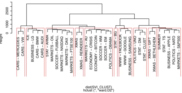
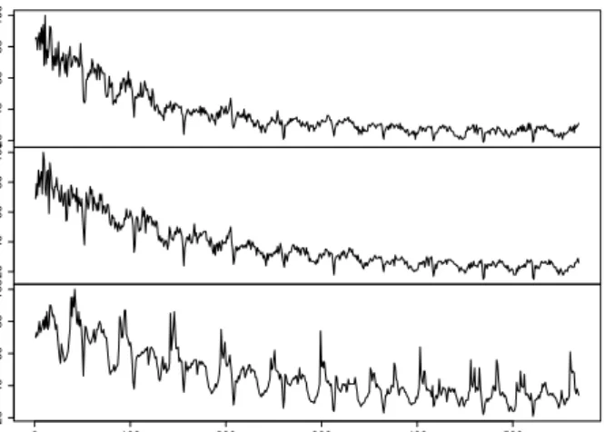
Clustering of unlabeled data is one important step in the pattern discovery process. In the machine learning jargon, clustering is assigned to unsupervised or semisupervised learning algorithms depending on whether we have hyperparameters or not. The aim of clustering is to find natural groupings in the data at hand. Thenatural groups are desired to be homoge-neous groups and found by maximizing the dissimilarity between groups and minimizing the dissimilarity within the groups. Apparently, similarity measures (see Section 3.5) are required for the clustering of time series. Figure 6 shows the Euclidean distance based hierarchical clustering for weekly Google search volume index data. The clusters of similar time series are marked by red rectangles and one exemplary cluster is the rectangle containing the SVIs for the query terms “Data Mining”, “Clustering” and “UNO”. Figure 7 shows these three SVIs which are detected as one cluster and indeed, the pathways look similar. Moreover, the closeness of the query terms “Data Mining” and “Clustering” are intuitively evident.
For static data, plenty of clustering approaches exist. Not all clustering procedures for static data can be overtaken or translated into the task of finding groups of similar time series. Only three major classes of clustering approaches are utilized for time series cluster-ing: hierarchical, partitioning and model-based methods. Hierarchical clustering operates in a bottom-up way as it merges similar clusters beginning with pairwise distances. A strong shortfall of hierarchical clustering is the limited number of time series we can cluster as the computational complexity is O(n2). Partitional clustering aims to minimize the sum of
CARS − MERCEDES CARS − VW ICE B USINESS − LG CARS − BMW CARS − A UDI ST A T − ARMA MARKETS − OIL SOCCER − FUßBALL MARKETS − NASD A Q MARKETS − D AX MARKETS − FTSE100 XMAS XMAS − REINDEER MARKETS − A U ECONOMY − CRISIS ECONOMY − BITCOIN SOCCER − WM SOCCER − EM POLITICS − OBAMA ST A T − BG WWW − F A CEBOOK WWW − GOOGLE B USINESS − SAMSUNG POLITICS − UNO ST A T − DM ST A T − CLUST XMAS − GIFT XMAS − BETHLEHEM SUMMER ST A T − TS B USINESS − APPLE POLITICS − NA T O MARKETS − S&P500 0 1000 2500
hclust (*, "ward.D2")dist(SVI_CLUST)
Height
Figure 6: Hierarchical clustering based on Euclidean Distances for weekly Google SVI data (01/2004 - 11/2014) on 34 different query terms. TSDMClust
squared errors within one cluster usingk-means. But, using ak-means algorithm, we have to prespecify the number of clusters kin this semisupervised learning procedure. Many differ-ent partitional clustering methods were proposed in recdiffer-ent years. For example Vlachos et al. (2003b) focus on k-means clustering and Cormode et al. (2007) implement k-center cluster-ing. M¨oller-Levet et al. (2003) focus on fuzzy clustering of short time series as they modify the fuzzy c-means algorithm for time series. Lin et al. (2004) adopt the multi-resolution property of wavelets for a partitioned clustering algorithm. Dai and Mu (2012) especially tailor the k-means clustering approach to a symbolic time series representation. Moreover, Rakthanmanon et al. (2011) focus on clustering of streaming time series data and for this purpose utilize the computational learningMinimum DescriptionLength (MDL) framework from Rissanen (1978).
Another general clustering idea stems from artificial neural networks and areSelfOrganizing
Maps (SOM) by Kohonen (2001). Euliano and Principe (1996) and Ultsch (1999) adopted SOM for time series and use self-organizing feature maps.
Lastly, model-based methods are frequently used clustering approaches. The most commonly known time series model is theAutoRegressiveIntegratedMovingAverage (ARIMA) model. For example Kalpakis et al. (2001) cluster ARIMA time series. An ARMA mixture model for time series clustering is proposed by Xiong and Yeung (2004). They derive an
expec-tation maximization approach for learning the mixing coefficients and model parameters. Moreover, HMM approaches are popular in time series clustering and pattern recognition applications. Panuccio et al. (2002), Law and Kwok (2000) as well as Bicego et al. (2003) develop HMM-based approaches for sequential clustering. Shalizi et al. (2002) uses HMM for pattern recognition as well, but they make no a priori assumptions about the causal archi-tecture of the data but starting from a minimal structure, they refer the number of hidden states and their transition structure from the data. Ge and Smyth (2000) model the distance between segments deformable Markov model templates and address hereby the problem of au-tomatic pattern matching between time series. Oates et al. (1999) introduce an unsupervised clustering approach of time series with hidden Markov models and DTW (see Section 3.5.1). They aim at an automatic detection ofK, the number of generating HMMs and learning the HMM parameters. For this purpose, they use the DTW similarity as an initial estimate of K. Related to model-based clustering methods, Wang et al. (2006) describe a characteristic-based clustering approach for time series data, i.e. they cluster time series with respect to global features extracted from the data. Additionally, Denton (2005) proposes a Kernel-based clustering approach for time series subsequences. However, Denton et al. (2009) show that its performance degrades fast for increasing window sizes. Lastly, Fr¨ohwirth-Schnatter and Kaufmann (2008) useMarkovChainMonte Carlo (MCMC) methods for estimating the ap-propriate grouping of time series simultaneously. For a more detailed review on time series clustering methods, please refer for example to Liao (2005) or Berkhin (2006).
In the context of time series data mining, the most common shortfall of time series cluster-ing techniques is the inability to handle longer time series. Keogh and Lin (2005) even claim that clustering of time series can be meaningless with randomly extracted clusters. Chen (2005) however argue against that claim using other similarity measures than the Euclidean distance as Keogh and Lin (2005) do. Time series increase mostly linear with time and this slows the pattern discovery process exponentially down (Fu, 2011). These facts plead again for the previously discussed preprocessing methods (Section 3). An effective compression of the data speeds up all subsequent tasks.
4.2 Knowledge Discovery: Pattern Mining
Generally speaking, knowledge discovery is referred to as the detection of frequently ap-pearing patterns, novelties and outliers or deviants in a time series database. Novelties are referred to anomalies or surprising patterns. Pattern discovery (or ’motif discovery’) comes
20 40 60 80 100 DM 20 40 60 80 100 CLUST 20 40 60 80 100 0 100 200 300 400 500 UNO Time
Figure 7: Three exemplary Google SVI time series detected to be similar according to hierarchical clustering on the query terms: “UNO”, “Clustering” and “Data Mining”
TSDMClust
along hand in hand with clustering methods as the occurrence frequency of patterns in time series subsequences can naturally be found by clustering.
As a general rule,motifs are seen as frequently appearing patterns in a time series database (Patel et al., 2002). Frequently appearing patterns are subsequences of time series which are very similar to each other. In recent years, motif mining in time series is of ever growing importance. Therefore, the available literature and approaches are manifold.
The most popular pattern discovery algorithm is from Berndt and Clifford (1994) and uses
Dynamic Time Warping (DTW, see Section 3.5.1). They use a dynamic programming ap-proach for this knowledge discovery task. Yankov et al. (2007) propose a motif discovery algorithm which is invariant to uniform scaling (stretching of the pattern length) and Chiu et al. (2003) approach time series motif discovery in a probabilistic way as they aim to cir-cumvent the inability to discover motifs in the presence of noise and poor scalability. Lonardi and Patel (2002) address the problem of finding frequently appearing patterns which are previously unknown. Most motif discovery approaches require a predefined motif length pa-rameter. Nunthanid et al. (2012) and Yingchareonthawornchai et al. (2013) approach this problem and propose parameter free motif discovery routines. Heading in a similar direction, Li et al. (2012) focus on the visualization of time series motifs with variable lengths and no a priori knowledge about the motifs. Moreover, Hao et al. (2012) rely on visual motif discovery, too. As time series can hide a high variety of different recurring motifs, they aim to support
visual exploration.
The importance of motif discovery techniques which can handle multivariate time series is ever growing. Papadimitriou et al. (2005) developed the popularStreamingPattern dIscoveRy in multIpleTime series (SPIRIT) algorithm which can incrementally find correlations and hid-den variables summarizing the key trends of the entire multiple time series stream. Tanaka et al. (2005) adduce the Minimum Description Length (MDL) principle and further use
Principal Component Analysis (PCA) for the extraction of motifs from multi-dimensional time series.
Naturally, many time series datasets have an inherent periodic structure. Therefore, de-tecting periodicity is another classical pattern discovery task. Besides classical time series analysis methods for handling seasonality and periodicity (see for example Brockwell and Davis (2009)), time series data mining community produced techniques for massive data sets. Han et al. (1998) and Han et al. (1999) address mining for partial periodic patterns as in many data applications full periodic patterns appear not that frequently. Elfeky et al. (2005) aim to mine for the periodicity rate of a time series database and Vlachos et al. (2004) use power spectral density estimation for the periodic pattern detection. Similarly, the de-tection of trends is a classical time series analysis task as well (see for example Brockwell and Davis (2009)). However, the detection of trend behavior is here subsumed under general pattern detection tasks described in this chapter. Only a few time series data mining papers explicitly address the identification of frequently appearing trends like for example Indyk et al. (2000) or Udechukwu et al. (2004).
Besides, a great assemblage of pattern discovery approaches are developed especially for fi-nancial time series data. The overall goal of all these papers is obvious: they want to forecast financial operating numbers. Lee et al. (2006) transfer financial time series data to fuzzy patterns and model them with fuzzy linguistic variables for pattern recognition. Fu et al. (2001) use self-organizing maps for pattern discovery in stock market data.
The massive amount of recently proposed motif discovery approaches for time series data mining reveals the yet unsatisfied demand for suitable techniques. For example the first al-gorithms for exact discovery of time series motifs are delivered by Mueen et al. (2009a) and Mueen et al. (2009b). Floratou et al. (2011) utilize suffix-trees to find frequent occurring patterns. Another more innovative approach is the particle swarm based multimodal opti-mization algorithm by Serr`a and Arcos (2015). Particle swarm is an computational optimizer and for example Kennedy (2010) provides more details on it.