Abstract - In logistics management, the use of vehicles to distribute products from suppliers to customers is a major operational activity. Optimizing the routing of vehicles is crucial for providing cost-effective services to customers. This research addresses the fleet size and mix vehicle routing problem (FSMVRP), where the heterogeneous fleet and its size are to be determined. A group genetic algorithm (GGA) approach, with unique genetic operators, is designed and implemented on a number of existing benchmark problems. GGA demonstrates competitive performance in terms of cost and computation time when compared to other heuristics.
Keywords - Logistics, vehicle routing, genetic algorithms
I. INTRODUCTION
In most supply chains, the management of distribution activities is a major operational task because distribution costs contribute a significant portion of the total operational costs. The need for effective distribution systems continues to come up in the supply chain industry due to escalating fuel costs. Distribution is a major part of logistics and a substantial cost to many companies. An effective distribution system can save millions of dollars each year. It can assist the decision maker in long-range planning, contract negotiations, and operations improvement. Hence, the development of effective and efficient distribution management systems is imperative.
In logistics industry, firms often require their vehicles to serve networks of hundreds of customers at various locations. As such, planning and scheduling can consume much time and effort, yet with little or no realizable cost efficiency. Several questions naturally arise: How many vehicles are needed to accommodate customer demand? What are the required vehicle capacities? What are the best routes? How best can customer demands be satisfied at the least possible cost? Due to multiple potential combinations of vehicle types and routing patterns, solutions to these questions are complex. This problem is a variant of the vehicle routing problem (VRP) [1].
The rest of the paper is as follows: Section II gives a brief outline of the VRP. Section III describes the fleet size and mix VRP (FSMVRP). A group genetic algorithm is proposed in Section IV. Computational tests and results are given in Section V. Section VI concludes the paper.
II. THE VEHICLE ROUTING PROBLEM
The VRP, first studied by Dantzig and Ramser [1], mainly seeks to minimize transportation costs, number of vehicles used, and customer waiting times. Since its inception in the 1950s, other VRP variants followed. The capacitated VRP (CVRP) is concerned with optimizing the dispatch of goods required by customers, using a fleet of capacitated homogenous vehicles [2]. Another variant is VRP with time window constraints (VRPTW), where arrival after the latest time window is penalized [3]. VRP problems with heterogeneous vehicles are frequently encountered in logistics industry. The heterogeneous fixed fleet VRP (HFFVRP) is a CVRP variant with a fixed number of available vehicles. The decision involves how best to utilize the existing vehicle fleet [4]. On the other hand, the FSMVRP is a CVRP variant where the fleet size and its composition are to be determined [5].
III. THE FSMVRP PROBLEM DISCRIPTION
Formally, the FSMVRP can be described as follows. There are n customer locations, {1, 2,..., n}. A fleet of T
vehicle types are available at the depot, represented by 0. The number of vehicles for each type is unlimited, and one of the decisions is to determine the number of vehicles of each type. Each vehicle type t has a capacity
Qt, a fixed cost ft and a variable cost per unit distance vt. Assume that between two vehicle types a and b, we have
fa fb if Qa Qb. Two cost structures exist: (i) different fixed costs with uniform variable costs [4-9], and (ii) different variable costs with no fixed costs [10-12]. For the FSMVRP with fixed costs and uniform variable costs;
t f
vt 1; t 0
(1)
For the FSMVRP with variable costs and no fixed costs;
t f
vt 0; t 0 (2)
Each customer node i 0 has a non-negative demand
di. Let the travelling distance between location i and j be non-negative τi,j. These distances are symmetric and satisfy the inequality, τi,j = τj,i and τi,jτj,k≥τi,k. Thus, the total variable cost of travelling from location i to location
j is vtτi,j. The FSMVRP consists in determining the vehicle fleet composition and the route of each vehicle, so that the total cost of delivering goods to all customers is minimized; each route starts and ends at the depot; each customer is visited exactly once; customer demands are 2Department of Quality and Operations Management, University of Johannesburg, Johannesburg, South Africa
satisfied; and vehicle capacity is not violated. Owing to FSMVRP complexity, the use of exact methods on large-scale instances is not viable. Not surprisingly, most approaches rely on heuristics that obtain good solutions, including tabu search [6] [7], memetic algorithm [11], genetic algorithm [11], particle swarm optimization [14], and evolutionary algorithm [12]. We propose a group genetic algorithm (GGA) to address the FSMVRP.
IV. GROUP GENETIC ALGORITHM APPROACH
We describe GGA and its elements, including chromosome coding, initialization, and genetic operators.
A. GGA Coding Scheme
The GGA performance strongly depends on the type of the coding scheme used. While most authors use depot(s) as trip delimiters [11] [12], a few do not use delimiters [15]. We develop our coding scheme from the later. The evaluation of a chromosome k = [1, 2, 3,…, n] involves partitioning customer orders along k into groups so that the cumulative load for each group does not exceed the vehicle capacity, and the cumulative delivery cost incurred is minimized. This is represented by a graph,
G(X) with vertex V(G) = {i | 0 ≤i ≤n}. Let E(G) be the set of directed arcs on G(X), where (i,j) E(G) iff
,
1 t
j i
m dm Q
and t be the vehicle type chosen. Eacharc (i,j) represents a feasible trip, where the vehicle departs from node 0 (depot) and visits nodes i+1, i+2,…,
j-1, and j, consecutively. The total load for trip (i,j) is given by
mji1dm.The objective is to select a vehicle type t with the least cost and capacity not less than the trip load. Then, for the FSMVRP with fixed cost, trip cost ci,j is equivalent to fixed cost plus variable costs [5];
1 1 , 1 ,0 1 , 0 , j i h hh j i t j i f c (3)
On the other hand, for the FSMVRP with no fixed cost;
t j i h hh j i j i v c
1 1 , 1 ,0 1 , 0 , (4)
Fig. 1. Typical data for chromosome representation
Consider a typical distribution center with T = 2 unlimitedvehicle types to serve n = 6retailers (see Fig. 1). The numbers on arc(i,j) and node j represent τi,j and di, respectively. The capacities of vehicle types t1 and t2 are
Q1 = 500 and Q2 = 550, respectively. Their fixed costs are
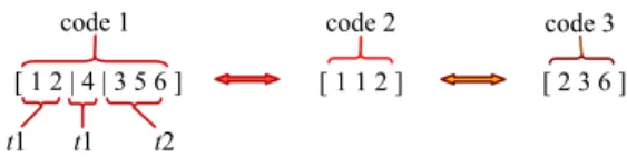
f1 = 300 and f2 = 400, respectively. The proposed GGA uses a group structure for each feasible solution based on three codes (see Fig. 2). Code 1, of size n, is a group structure upon which the genetic operators act. Code 2 shows the vehicle type assigned to each trip, while code 3 represents the position of the last node of each trip.
Fig.2. Chromosome representation
The chromosome [1 2 4 3 5 6 · 1 1 2], comprises codes 1 and 2 (“·” demarcates codes 1 and 2). According to code 1, vehicle type 1, with f1 = 300 and vt = 1, is assigned trip (0-1-2-0). From (3) the total cost for this trip is 300 + 240 + 42 + 280 = 862. Other trips, (0-4-0) and (0-3-5-6-0), are evaluated in a similar manner, as shown in Table I.
TABLE I.
GGA CODING SOLUTION EXAMPLE
Trip Vehicle type Cost
0-1-2-0 1 862
0-4-0 1 700
0-3-5-6-0 2 930
Total Cost 2492
B. Initialization
An initial population of the desired size, popsize, is produced by (i) savings [16] and sweep heuristics [17], and (ii) random generation. The savings algorithm is applied using one vehicle type at a time. The sweep algorithm is also used to generate initial solutions. These initial solutions are then concatenated into chromosomes. More chromosomes are generated as follows;
Repeat
1. Assign a location to each vehicle t, (t = 1,2,…, m) 2. Randomly assign the remaining locations, 3. Encode the string and add to initial population,
Until (population size = popsize).
The GGA approach minimizes some cost function f
which is mapped to a score function, as suggested in [23];
)] ( , 0 max[ ) ( max k k f g f (5)
where, gk(τ) is the objective function of chromosome k at time τand fmax is the largest objective function.
C. Selection Operator
Several selection strategies have been suggested by Goldberg [18], including deterministic sampling, remainder stochastic sampling with/without replacement, and stochastic tournament. The remainder stochastic
[ 1 2 | 4 | 3 5 6 ] [ 1 1 2 ] t1 t1 t2 [ 2 3 6 ] code 3 code 1 code 2 0 300 42 280 20 120 250 320 200 70 20 100 270 240 4 2 3 1 5 6 50 500 100 Vehicle t1: Q1 = 500, f1 = 300; Vehicle t2: Q2 = 550, f2 = 400 500
sampling without replacement is applied in this work; each chromosome k is selected and stored in the mating pool according to its expected count ek calculated thus;
popsie k k k k f popsize f e 1 1 (6)Here, fk is the score function of the kth chromosome. Each chromosome receives copies equal to the integer part of ek, that is, [ek], while the fractional part frac(ek) is treated as a success probability of obtaining additional copies of chromosome k into the mating pool.
D. Crossover Operator
Crossover is an evolutionary mechanism by which selected chromosomes mate to produce new offspring, called selection pool. This enhances exploration of unvisited regions in the solution space. The proposed group crossover operator exchanges groups of genes of selected chromosomes (see Fig.3), with probability
prcoss, until the desired pool size, poolsize,is obtained:
Repeat
1. Generate the crossover point in (1, g-1), g = trips. 2. Swap the groups to the right of the crossover point. 3. Repair the offspring, if necessary.
Until (selection poolsize is achieved).
Fig. 3: Crossover operator
After crossover, some customers may appear in more than one trip, while others may be missing. Such offspring should be repaired by eliminating duplicated customers to the left of the crossover point (see Fig.4) and inserting missing ones into the trip with the least loading. Thus, group coding takes advantage of the group structure. The basic single-point crossover is applied on code 2.
Fig. 4: Chromosome repair mechanism E. Mutation Operator
Mutation is applied to every new chromosome using two mutation operators; swap mutation and shift mutation. The swap mutation operates by exchanging genes between two groups in a chromosome according to the following procedure:
1.Randomly select two numbers from set {1, 2,…,g}; 2.Randomly choose a gene from each group;
3.Swap the selected genes.
Fig. 5 illustrates the swap mutation mechanism.
Fig. 5. Swap mutation
The shift mutation works by shifting the frontier between two adjacent groups by one step, either to the right or to the left (see Fig. 6) as follows;
1. Randomly generate the frontier in (1, g-1). 2. Randomly choose the shift direction: right or left. 3. Shift the frontier in the selected direction.
Figure 6: Shift mutation operator
As for the genes that correspond to code 2, a basic mutation operator is applied by replacing a randomly selected gene with a randomly generated integer in {0, 1,…,T}. Mutation essentially provides GGA with a local search capability, called intensification. However, shift mutation is a more localized search than swap mutation.
F. Inversion Operator
To curb premature convergence, inversion is applied at a low probability on selected chromosomes. Inversion rearranges chromosome groups in a reverse order (Fig. 7).
Before inversion : [ 1 2 | 4 | 3 5 6 ] After inversion : [ 3 5 6 | 4 | 1 2 ]
Fig. 7: Inversion operator G. Diversification
As iterations proceed, the population converges to a particular solution. Premature convergence may occur before an optimal solution is obtained. To check diversity, define an entropic measure Hi for each location i;
m j ij ij i m opsize p n popsize n H 1 log( ) ) ( log ) ( (7)where nij is the number of chromosomes in which location
i is assigned position j in the current population; m is the number of locations. Then, diversity H is defined as,
m i i m H H 1 (8) Offspring chromosome : [ 1 2 | 4 | 3 5 6 ] Select group or trip : 2 and 3 Select genes or nodes : 4and 6 Mutated offspring : [ 1 2 | 6 | 3 5 4offspring chromosome : [ 1 2 | 4 | 3 5 6 ] select frontier, rand (1,2) : 1
select direction : left mutated offspring : [ 1 | 2 4 | 3 5 shift frontier Before repair: [ 1 2 | 4| 4 6 ] [ 1 2 | - | 4 6 ] After repair: [ 1 2 | 3 5 | 4 eliminate 4 introduce 3,5 [ 1 2 | 4 | 3 5 6 ] [ 1 2 | 4 | 4 6 ] swap [ 1 3 | 2 5 | 4 6 ] [ 1 3 | 2 5 | 3 5 6 ] Parents: Offsprings:
Therefore, inversion is applied to improve diversity to a desired value. The best candidates from diversified and
undiversified populations are always preserved. G. The GGA Implementation
The overall GGA (Fig. 8) incorporates the operators described in previous sections, using carefully chosen genetic probabilities: crossover (0.4), mutation (0.01), and inversion (0.05) as in [21].
GGA Algorithm: BEGIN
1: Input: initial data input: select GGA parameters; 2: Initial population, oldpop: create chromosomes;
(i) savings and sweep algorithms; then, (ii) random generation; Repeat
3: Selection/recombination:
(i) evaluate strings by fitness function;
(ii) create temporal population, temppop: use int [ek], then frac(ek) 4: Groupcrossover/recombination:
(i) select 2 strings by selection strategy from temppop. (ii) apply crossover operator to the 2 strings. (iii) if successful, apply inversion, else go to 5. (iv) apply repair mechanism if necessary.
5: Mutation: mutate and move offspring to new population, newpop; 6: Replacement strategy:
(i) compare selection pool spool and oldpop strings, successively; (ii) take the one that fares better in each comparison;
(iii) select the rest of the strings with probability 0.55; 7: Diversification:
(i) calculate population diversity H; (ii) if (H Hmin) then diversify till H ≥Hmin;
(iii) re-evaluate strings by fitness function; 8: New population:
(i) oldpop = newpop
(ii) advance population, gen = gen + 1 Until (gen ≥maxgen)
END
Fig. 8: Proposed GGA Implementation
V. COMPUTATIONAL TESTS AND DISCUSSIONS
A. Problem Sets
The proposed GGA was implemented in Java and executed on a Pentium 4 at 3GHz based on 12 benchmark problems in [20]. Table II specifies the costs, vehicle capacity Qt, (t = 1, 2,…, 6); fixed cost ft; and variable cost
vt. Using the notation in [5], problem sets 3 to 6 have 20 customers, 13 to 16 have 50, 17 to 18 have 75, and 19 to 20 have 100. Computational results were compared with those from best-performing heuristics in the literature, including tabu search [21] [7] [9], column generation-based heuristics [8], and evolutionary algorithm [12].
B. Computations, Results and Discussions
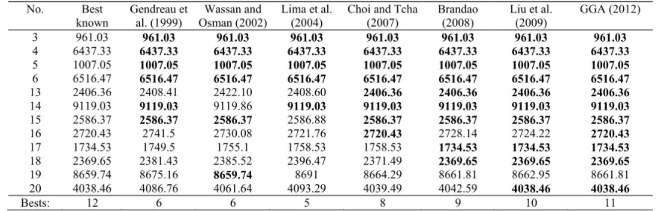
Table III presents the computational results of the FSMVRP with fixed costs. A count of the best-known solutions obtained by the heuristics is provided. Out of the 12 benchmark problems, our GGA approach produced 11 best known solutions, compared to only 6 found in [21], 6 in [7], 5 in [15], 8 in [8], 9 in [9], and 10 in [5].
Table IV presents the percentage deviation of each solution from the best-known and the computation times for each problem. All algorithms showed remarkable accuracy, with average percent deviation less than 1%. Our GGA performed competitively in terms of percentage deviation and computation times. The results demonstrate the utility of the GGA developed in this research.
VI. CONCLUSIONS AND FURTHER RESEARCH TABLE II
SPECIFICATIONS FOR THE BENCHMARK PROBLEMS
No. Q1 f1 v1 Q2 f2 v2 Q3 f3 v3 Q4 f4 v4 Q5 f5 v5 Q6 f6 v6 3 20 20 1.0 30 35 1.0 40 50 1.0 70 120 1.0 120 225 1.0 4 60 1000 1.0 80 1500 1.0 150 3000 1.0 5 20 20 1.0 30 35 1.0 40 50 1.0 70 120 1.0 120 225 1.0 6 60 1000 1.0 80 1500 1.0 150 3000 1.0 13 20 20 1.0 30 35 1.1 40 50 1.2 70 120 1.7 120 225 2.5 200 400 3.2 14 120 100 1.0 160 1500 1.1 300 3500 1.4 15 50 100 1.0 100 250 1.6 160 450 2.0 16 40 100 1.0 80 200 1.6 140 400 2.1 17 50 25 1.0 120 80 1.2 200 150 1.5 350 320 1.8 18 20 10 1.0 50 35 1.3 100 100 1.9 150 180 2.4 250 400 2.9 400 800 3.2 19 100 500 1.0 200 1200 1.4 300 2100 1.7 20 60 100 1.0 140 300 1.7 200 500 2.0 TABLEIII
COMPUTATIONAL RESULTS FOR THE BENCHMARK PROBLEMS No. Best known Gendreau et al. (1999) Wassan and Osman (2002) Lima et al. (2004)
Choi and Tcha (2007) Brandao (2008) Liu et al. (2009) GGA (2012) 3 961.03 961.03 961.03 961.03 961.03 961.03 961.03 961.03 4 6437.33 6437.33 6437.33 6437.33 6437.33 6437.33 6437.33 6437.33 5 1007.05 1007.05 1007.05 1007.05 1007.05 1007.05 1007.05 1007.05 6 6516.47 6516.47 6516.47 6516.47 6516.47 6516.47 6516.47 6516.47 13 2406.36 2408.41 2422.10 2408.60 2406.36 2406.36 2406.36 2406.36 14 9119.03 9119.03 9119.86 9119.03 9119.03 9119.03 9119.03 9119.03 15 2586.37 2586.37 2586.37 2586.88 2586.37 2586.37 2586.37 2586.37 16 2720.43 2741.5 2730.08 2721.76 2720.43 2728.14 2724.22 2720.43 17 1734.53 1749.5 1755.1 1758.53 1758.53 1734.53 1734.53 1734.53
FSMVRP involves the determination the fleet size and the mix of heterogeneous vehicles, assuming that the number of vehicles of each type is unlimited. This paper presents a GGA for solving the FSMVRP with fixed and variable costs. The approach obtained best-known solutions based on the comparative analysis tests on benchmark problems. Moreover, the GGA approach performed competitively within a reasonable computation time. In terms of the average solution cost, GGA demonstrated competitive performance.
This research contributes logistics and transportation. The current GGA uses unique group genetic operators, demonstrating its competitive performance when compared to related approaches in the literature. Possible further research directions include the design of more efficient algorithms for solving the FSMVRP problem in which the customer demand is uncertain or fuzzy.
REFERENCES
[1] G. B. Dantzig and J. H. Ramser. “The Truck Dispatching Problem,” Management Science, vol. 6, pp. 80-91, 1959. [2] P. Toth and D. Vigo, “The Vehicle Routing Problem,”
SIAM Monograph on Discrete Mathematics and Applications, Philadelphia, PA: SIAM, 2002.
[3] O. Braysey, and M. Gendreau, “Vehicle routing problems with time windows, part I: Route Construction and Local Search Algorithms,” Transportation Science, vol. 39, no. 1, pp. 104–118, 2005.
[4] E.D Taillard. “A heuristic column generation method for the heterogeneous fleet VRP,”. RAIRO 33, pp. 1–34, 1999. [5] S. Liu, W. Huang and H. Ma. “An effective genetic
algorithm for the fleet size and mix vehicle routing problems,” Transportation Research Part E, vol. 45, pp. 434-445, 2009.
[6] M. Gendreau, G. Laporte, C. Musaraganyi, and E.D. Taillard, “A tabu search heuristic for the heterogeneous fleet vehicle routing problem,” Computers and Operations Research, vol. 26, pp. 1153–1173, 1999.
[7] N.A. Wassan and I.H. Osman, “Tabu search variants for the mix fleet vehicle routing problem,” Journal of the Operational Research Society, Vol. 53, pp. 768–782, 2002 [8] E. Choi and D.W. Tcha. “A column generation approach to
the heterogeneous fleet vehicle routing problem,” Computers and Operations Research, vol. 34, pp. 2080– 2095, 2007.
[9] J. Brandao. “A deterministic tabu search algorithm for the fleet size and mix vehicle routing problem,” European Journal of Operational Research, vol. 195 No. 3, pp. 716-728, 2008.
[10] I. Osman, S. Salhi, “Local search strategies for the vehicle fleet mix problem,” In: Rayward-Smith, V.J., Osman, I.H., Reeves, C.R., Smith, G.D. (Eds.), Modern Heuristic Search Methods. Wiley, New York, pp. 131–153, 1996.
[11] C.M.R.R. Lima, M.C. Goldbarg, E.F.G. Goldbarg. “A memetic algorithm for the heterogeneous fleet vehicle routing problem,” Electronic Notes in Discrete Mathematics, vol. 18, pp. 171–176, 2004.
[12] L.S. Ochi, D.S. Vianna, L.M. Drummond, A.O. Victor. “A parallel evolutionary algorithm for the vehicle routing problem with heterogeneous fleet,” Future Generation Computer System, vol. 14, pp. 285–292, 1998.
[13] C.D. Tarantilis, C.T. Kiranoudis, V.S. Vassiliadis, “A threshold accepting metaheuristic for the heterogeneous fixed fleet vehicle routing problem,” European Journal of Operational Research, vol. 152, pp. 148–158, 2004. [14] B. F Moghadam and S. M. Seyedhosseini, “A particle
swarm approach to solve vehicle routing problem with uncertain demand: A drug distribution case study,” International Journal of Industrial Engineering Computations, vol. 1, pp. 55-66, 2010
[15] C. Prins. “A simple and effective evolutionary algorithm for the vehicle routing problem,” Computers and Operations Research, vol. 31, pp. 1985–2002, 2004
[16] G. Clarke, J.W. Wright. “Scheduling of vehicles from a central depot to a number of delivery points,” Operations Research, vol. 12, pp. 568–581, 1964.
[17] B. Gillett, L. Miller. “A heuristic for the vehicle dispatching problem,” Operations Research, vol. 22, pp. 340–349, 1974.
[18] D. E. Goldberg, Genetic Algorithm in Search, Optimization, and Machine Learning, Addison-Wesley, Reading, MA, 1989.
[19] E.V. G. Filho and A.J. Tiberti. “A group genetic algorithm for the machine cell formation problem,” International Journal of Production Economics, Vol 102, pp. 1-21, 2006. [20] B. Golden, A. Assad, L. Levy and F. Gheysens. “The fleet
size and mix vehicle routing problem,”. Computers and Operations Research, vol. 11, pp. 49–66, 1984.
M. Gendreau, G. Laporte, C. Musaraganyi and E.D. Taillard. “A tabu search heuristic for the heterogeneous fleet vehicle routing problem,“. Computers and Operations Research, vol. 26, pp. 1153–1173, 1999.
No. Best known
Gendreau et al. (1999) Lima et al. (2004) Choi and Tcha (2007) Liu et al. (2009) GGA (2012) Deviation Time (s) Deviation Time (s) Deviation Time (s) Deviation Time (s) Deviation Time (s)
3 961.03 0.000 164 0.000 89 0.000 0 0.000 0 0.000 0 4 6437.33 0.000 253 0.000 85 0.000 1 0.000 0 0.000 1 5 1007.05 0.000 164 0.000 85 0.000 1 0.000 2 0.000 2 6 6516.47 0.000 309 0.000 85 0.000 0 0.000 0 0.000 0 13 2406.36 0.085 724 0.093 559 0.000 10 0.000 91 0.000 89 14 9119.03 0.000 1033 0.000 669 0.000 51 0.000 42 0.000 65 15 2586.37 0.000 901 0.020 554 0.000 10 0.000 48 0.000 55 16 2720.43 0.775 815 0.049 507 0.000 11 0.139 107 0.000 10 17 1734.53 0.863 1022 1.384 1517 1.384 207 0.000 109 0.000 113 18 2369.65 0.497 691 1.132 1613 0.078 70 0.000 197 0.000 211 19 8659.74 0.178 1687 0.361 2900 0.053 1179 0.037 778 0.024 804 20 4038.46 1.196 1421 1.358 2383 0.026 264 0.000 1004 0.000 1047 Averages: 0.3012% 776.9 0.3171% 887.4 0.1462% 172.4 0.0176% 209.0 0.0024% 209.7