Accepted Manuscript
Adaptive low-level control of autonomous underwater vehicles using deep reinforcement learning
Ignacio Carlucho, Mariano De Paula, Sen Wang, Yvan Petillot, Gerardo G. Acosta
PII: S0921-8890(18)30151-9
DOI: https://doi.org/10.1016/j.robot.2018.05.016
Reference: ROBOT 3039
To appear in: Robotics and Autonomous Systems
Received date : 22 February 2018 Revised date : 2 May 2018 Accepted date : 30 May 2018
Please cite this article as: I. Carlucho, M. De Paula, S. Wang, Y. Petillot, G.G. Acosta, Adaptive low-level control of autonomous underwater vehicles using deep reinforcement learning,Robotics and Autonomous Systems(2018), https://doi.org/10.1016/j.robot.2018.05.016
This is a PDF file of an unedited manuscript that has been accepted for publication. As a service to our customers we are providing this early version of the manuscript. The manuscript will undergo copyediting, typesetting, and review of the resulting proof before it is published in its final form. Please note that during the production process errors may be discovered which could affect the content, and all legal disclaimers that apply to the journal pertain.
Adaptive low-level control of autonomous underwater vehicles
using deep reinforcement learning
Ignacio Carluchoa,b, Mariano De Paulaa1, Sen Wangb, Yvan Petillotb, Gerardo G. Acostaa
aINTELYMEC group, Centro de Investigaciones en Física e Ingeniería del Centro CIFICEN – UNICEN – CICpBA –
CONICET, Argentina
bSchool of Engineering & Physical Sciences Heriot-Watt University, EH14 4AS, Edinburgh, UK
[email protected],[email protected], [email protected], [email protected], [email protected]
Abstract
Low-level control of autonomous underwater vehicles (AUVs) has been extensively addressed by classical control techniques. However, the variable operating conditions and hostile environments faced by AUVs have driven researchers towards the formulation of adaptive control approaches. The reinforcement learning (RL) paradigm is a powerful framework which has been applied in different formulations of adaptive control strategies for AUVs. However, the limitations of RL approaches have lead towards the emergence of deep reinforcement learning which has become an attractive and promising framework for developing real adaptive control strategies to solve complex control problems for autonomous systems. However, most of the existing applications of deep RL use video images to train the decision making artificial agent but obtaining camera images only for an AUV control purpose could be costly in terms of energy consumption. Moreover, the rewards are not easily obtained directly from the video frames. In this work we develop a deep RL framework for adaptive control applications of AUVs based on an actor-critic goal-oriented deep RL architecture, which takes the available raw sensory information as input and as output the continuous control actions which are the low-level commands for the AUV’s thrusters. Experiments on a real AUV demonstrate the applicability of the stated deep RL approach for an autonomous robot control problem.
Keywords: Autonomous robot; Deep Reinforcement Learning; AUV; Adaptive low-level control.
1. Introduction
Autonomous underwater vehicles are revolutionizing the oceanic research with applications on a vast number of scientific fields such as marine geoscience, biology and archeology but also in the private sector such as the oil and gas industry [1,2]. Over the years, there have been intensive efforts toward the development of autonomous control strategies for AUVs [3]. Autonomy implies that an entity can act independently according to its own criterion and it is an essential feature for engineering systems in large and uncertain environments [4]. In this sense, adaptive low-level control techniques have arisen as a way to provide autonomy to AUVs allowing them to operate in hostile environments [5].
Classical control theory has evolved in a variety of methods for low-level AUV control. Several versions of the well-known PID controller have been developed and used for AUV control. To name a few, in the early work of Jalving [6] a simple proportional derivative controller was proposed for AUV steering control. Fjellstad and Fossen [7] designed a PID controller for position and attitude tracking of an AUV and the global convergence of their proposal was proven by Barbalat’s lemma. More sophisticated proposals can be found in the work of Valenciaga, et al. [8] where a proportional integrative controller for multiple inputs and multiple outputs (PI-MIMO) was formulated to command the rudder and the propeller of an AUV. In the work of Sutarto and Budiyono [9] a linear parameter varying (LPV) control strategy based on linear fractional transformation to formulate a robust gain schedule strategy for robust longitudinal control of an AUV was developed. To deal with the AUV modeling uncertainties and the saturations of the control actions imposed by the AUV actuators, Sarhadi et al. [10], proposed an adaptive PID formulations with anti-windup compensators and then the stability was analyzed by Lyapunov theory and the proposed control technique was implemented in an onboard computer to be checked in a real-time dynamic simulation environment.
When model estimation accuracy could be imprecise and the system nonlinearities are considered, Lyapunov-based algorithms have many advantages for control formulations. An example can be found in Ferreira et al. [11] where several independent controllers have been developed, based only on Lyapunov theory, to perform decoupled motions of an AUV. In the work of Lapierre and Jouvencel [12] a nonlinear robust control formulation resorting to Lyapunov-based techniques was presented. In this case a virtual target principle was used to design an asymptotically convergent kinematic control, relying on a switching control strategy for the dynamic parameters. However, the disturbance rejection was not explicitly addressed in the formulation and the authors have explicitly recognized that further research is needed. In another way, developments coming from nonlinear control designs have been made where linear transformations were used to solve Linear Quadratic and Gaussian regulators (LQR and LQG, respectively) as in the work of Wadoo et al. [13] where a system linearization is carried out for the control of a the kinematic model of an AUV and then a LQG was formulated as a H-2 optimization problem. Geranmher et al. [14] considered a general fully coupled AUV and applied nonlinear suboptimal control, where the state-dependent Riccati equation was used to generate a suboptimal path solution. In the work of Fischer et al. [15] a continuous robust integral of the sign of the error control was used to compensate for uncertain, nonautonomous
disturbances for a coupled and fully-actuated underwater vehicle. Moreover, semiglobal asymptotic stability was proven by a Lyapunov-based stability analysis.
Underwater vehicle hydrodynamics are highly non-linear with uncertainties that are difficult to parameterize and, in addition, unknown disturbances are usually present as are typical of aquatic environments. For these reasons, researchers have resorted to adaptive controllers and have often included the dynamical model or have estimated the system parameters in the formulation of the controllers. Early, Fossen and Fjellstad [7] discussed the performance of the adaptive control laws for controlling underwater vehicles. Afterward, several adaptive PID formulations have been proposed as in works of Antonelli et al. [16] where different adaptive versions based on PID control laws were formulated with an adaptive compensation of the dynamics. However, in such proposals the control gains must be adjusted manually, first in simulation and then with the real system during its operation [17]. An adaptive on-line tuning method for a coupled two-loop proportional controller of four degrees-of-freedom for an autonomous underwater vehicle is presented in the work of Barbalata et al. [18] where the gains of each controller are determined on-line according to the error signals. Rout and Subudhi [19] developed an adaptive tuning method for a PID controller using an inverse optimal control technique based on a NARMAX model for the representations of the non-linear dynamics. Other adaptive feedback controller was proposed by Narasimhan and Singh [20] using LQR theory for the computation of the optimum feedback gain vector of the control system, in this case used for depth control of a low-speed underwater vehicle. These facts evidence a growing need for self-adapting controllers to environmental conditions.
To enhance the different control formulations researchers have turned their attention to artificial intelligence techniques to be incorporated in adaptive control formulations to develop real autonomous systems. Particularly, using artificial neural networks (ANNs) in AUV control formulations has the advantage that the dynamics of the AUVs do not need be fully known and ANNs can learn a full, or partial, model of the nonlinear dynamics which can in turn be used for the controller design [21]. In Shi et al. [22] a hybrid control approach for AUV depth control has been proposed using the Lyapunov theory approach for the synthesis of an adaptive controller and an ANN was employed to model the depth dynamics. A dual closed loop control system was proposed in [23] where a bio-inspired model for velocity control was used in an inner control loop and a sliding-mode controller was used in an outer tracking control loop which managed the position and orientation of an AUV. Also, a traditional Lyapunov stability analysis was carried out based on the AUV dynamic model. However, strong nonlinearities, as in underwater vehicles applications, make this analysis difficult. In this sense, after the development of the fuzzy logic many fuzzy control strategies were proposed for AUV control [24–27]. Briefly, fuzzy logic control makes a smooth approximation of a nonlinear system using a fuzzy inference system [28] consisting of a set of linguistic rules about the system behavior and membership functions which must be conveniently defined. In the work of Raeisy et al. [29] a simple fuzzy control formulation can be found with two fuzzy control loops, one that controlled the roll and yaw and the other the depth of the AUV, while incorporating an optimization procedure for the fuzzy parameters using the root mean square error between the input and the output as cost
function. Recently, Khodayari et al. [30] have proposed a self-adaptive fuzzy PID controller for the attitude control of an AUV based on its previously obtained dynamic model from mechanical principles. Also, fuzzy control formulations for underwater vehicle-manipulator system (UVMS) were formulated in Esfahani et al. [31]. However, one disadvantage for using fuzzy control systems for AUVs is that subjective knowledge is required for the definition of the fuzzy rules and membership functions.
Other important branch with growing importance in the field of artificial intelligence for autonomous control systems is the RL paradigm [32]. Instead of supervised learning as ANNs, RL is a mixed approach between supervised and unsupervised learning using actor-critic approach with potential advantages for adaptive control formulations in robotics [33,34]. In a nutshell, RL algorithms are able to learn a control policy through the interactions between the system and its environment. RL algorithms can be formulated as model-free and/or model-based [35,36]. The former uses the experience from interaction to determine directly the optimal control policy [32,37] while the latter uses it to learn/update the current model of the system or to improve the value function and/or the policy directly [38].
Particularly, for AUVs relevant works have been developed using RL formulations. In the early work of Gaskett et al. [39] a model-free RL algorithm was developed to control the thrusters responses of an AUV. More recently, Carreras et al. [40] proposed a hybrid behavior-based scheme using RL for high-level control of an AUV. In this work a semi-online neural-Q-learning algorithm was formulated using a multilayer neural network to learn the internal continuous state-action mapping of each behavior. In the work of El-Fakdi et al. [41] an on-line direct policy search algorithm based on a stochastic gradient descent method with respect to the policy parameter space was proposed. In this formulation, the policy was represented by a neural network, where its weights were the policy parameters. The states of the systems were the inputs to the neural network and the outputs were the action selection probabilities [42]. Then, El-Fakdi and Carreras [43] developed a simulation-based actor-critic algorithm using policy gradient method to solve a cable tracking task. In this formulation an initial policy is learned off-line using a hydrodynamic model of the AUV. Similarly, a two layered control architecture was proposed in [44], where an on-line RL algorithm selects the desired direction of the velocity of a marine vehicle and which, in turn, are the downstream references for a low-level proportional-derivative controller. In this work, only simulation results were reported using a computational dynamic model. In the work of Frost and Lane [45] an evaluative simulation analysis of the performance of the Q-learning algorithm for an AUV in search and inspect missions was performed using a discretized version of a continuous simulation environment to turn the problem into a grid-world type scenario. This study concluded in the need of improvements for the function approximation of the state space. In Frost et al. [46] a behavior-based architecture for AUV path planning using an actor-critic RL approach was developed. The proposed architecture regulates a set of weights of a behavior based module which, in turn, sets the control signals of the thrusters. Also, the adaptation capability of the propose approach was analyzed by a thruster failure-tolerant study for different fault scenarios. Cui et al. [47] proposed an adaptive trajectory tracking control for AUVs using a discrete dynamical model of the underwater vehicle integrated with two artificial neural network of radial basis functions, one of them used to
evaluate the long-time performance of the designed AUV control and the other is used to compensate the unknown dynamics. The weights of the ANN are adjusted by a standard formulation of a RL algorithm.
One of the major obstacles for RL formulations resides in dealing with applications in continuous state/action spaces when the use of function approximators is required to approximate the control policy and the state/action value functions [48,49]. Often, linear approximators are not suitable for complex systems and then nonlinear function approximators, like artificial neural networks, are required. However, the nonlinearity in ANNs may cause instabilities in the RL algorithms or may even diverge. From the developments of training algorithms for deep neural networks [50,51], Mnih et al. [52] introduced the deep Q-Network (DQN) which uses deep neural networks, i.e. Convolutional Neural Networks (CNN), to approximate the action-value function and have shown that the training of the Q function has been stabilized using experience replay and a target network. From this seminal contribution, deep RL has emerged as a modern research field and it has become an attractive and promising framework for developing real-time adaptive control strategies to formulate adaptive control proposals for autonomous systems However, the DQN algorithm can only be applied to discrete problems, that is, with finite discretized spaces of states and actions. Llicrap et al. [53] extended deep RL formulations for continuous state/action domains for what they developed the deep deterministic policy gradient (DDPG) algorithm based on the deterministic policy gradient (DPG) algorithm [54] incorporating the ideas of batch normalization [55] and experience replay as in [52].
Mostly, the proposed deep RL algorithms have been tested on simulated systems mainly using simulation environments as video games simulators. Yu et al. [56] implemented the DQN algorithm to learn to avoid obstacles by learning the turning actions for a simulated car using the raw video frame images as inputs, which are directly obtained from a video game simulator. Ganesh et al. [57] used TensorFlow [58] and Keras [59] software frameworks to train a fully-connected deep neural networks, as deep RL agent, to autonomously drive across a diverse range of track geometries using a 3D car racing simulator called TORCS (The Open Racing Car Simulator) which is a modern open source simulation platform used for research in control systems and autonomous driving [60]. Similarly, El Sallab et al. [61] proposed a deep learning algorithm for autonomous driving, incorporating recurrent neural networks and attention models to integrate the information and to focus on relevant information, respectively. This proposal was tested in TORCS with successful results and a good computational performance, which is an important feature for potential deployments on real robots. Specifically, for control applications of AUVs,Yu et al. [62] have solved, in a simulation environment, the trajectory tracking control problem of an AUV using a deep RL algorithm with two embedded neural networks, the actor deep neural network and the critic deep neural network. In the formulation, the DPG algorithm was used to update the critic function and the first-order gradient-based stochastic optimization method was used to update the weights of the actor function [63].
Particularly, during the literature review a non-significant amount of previous works in deep RL has been identified for continuous control applications and, even less so, to develop autonomous control strategies for underwater vehicles. In this work we propose a deep RL formulation with a deterministic actor-critic
architecture, mainly based on the DDPG algorithm [53], adapted for low-level control of an AUV using only its on-board sensors as perception system which, in turn, becomes the inputs for the control algorithm. The successful results obtained from real experiments using an underwater vehicle demonstrated the applicability of deep RL for robotics. In this way, the obtained results demonstrated the feasibility for deep RL to be applied on a real robot and also the encouraging results open a new promising avenue for the application of the deep RL paradigm in the engineering community and, specifically, to develop autonomous systems into the robotics field, such as AUVs.
The paper is structured as follows: In Section 2, we briefly introduce the necessary background on RL and the standard Q-learning algorithm as well as an overview to deep neural networks. In Section 3 we develop our proposed deep RL framework for AUV control. In Section 4, we provide experimental evidence of our proposal. Section 5 concludes the paper with the relevant contributions.
2. Background
In this section we give a non-exhaustive overview of the fundamentals of RL as well as the well-known Q-learning algorithm that form the basis for the subsequent deep RL developments. Following, the deterministic policy gradient method for RL formulations is summarized. Also, a brief and general overview of deep neural networks is presented which will be used as function approximators in deep RL formulations. These concepts are the basis for our proposed adaptive scheme for the low-level control of an underwater vehicle which will be developed in the next sections.
2.1. Reinforcement learning statement
The RL problem [32] consists in learning iteratively how to achieve a goal, or to accomplish a control task, from ongoing interactions with a real or simulated system. Commonly, in RL formulations the control problem is defined by four elements, namely, the state space , the action space , the state transition probability and the reward function ∙ .
In a control problem, at time , an action is a vector, , of selected values for the manipulated variables which could be the inputs to the system actuators. During the learning process, an artificial agent interacts with the system by taking an action, in our case, a new set of control actions ∈ ⊆ and, after that, the system evolves from the state ∈ ⊆ to and the agent receives a numerical signal called reward (or punishment) which provides a measure of how good (or bad) the action taken at was in terms of the observed state transition. Rewards are given as hints regarding goal achievement or optimal behavior. Thus, the objective of the RL methods is to obtain the optimal policy ∗ satisfying the Eq.(1), where is the expected total reward under the control policy . The main objective of an RL agent is to learn an optimal policy, ∗, which defines the optimal control actions ( ) for different system’s states ( ), bearing in mind both short and long term rewards.
∗ max max E | (1)
Let’s assume that under a given policy , the expected cumulative reward , or value function over a certain time interval, is a function of , where are the corresponding state values and
defines the policy-specific sequence of the agent’s actions. The sequence of state transitions gives rise to rewards . Robot control is a continuous task without a single final state
therefore the discounted sum of future rewards ⋯ ∑ is used to
define the (discounted) expected state-value function for a policy from the state , as:
| ∑ (2)
where ∈ 0,1 is the discount factor which weights future rewards. Similarly, the state-action value function is defined as:
Q , | , ∑ , (3)
When the agent starts in state and executes the optimal policy ∗, ∗ is used to denote the maximum discounted obtained reward. Thus, the associated optimal state-value function that satisfies the Bellman's equation for all state is:
∗ arg max . ∗ | , (4)
where ∗ . Similarly, the optimal state–action value function Q∗ is defined by:
Q∗ , . ∗ | , (5)
such that ∗ max Q∗ , for all . Once Q∗is known through interactions, then the optimal policy can be obtained directly through:
∗ arg max Q∗ , (6)
2.2. RL in continuous domain: AUV low-level control
The previously exposed Q learning method results in an adaptive control algorithm that converges on-line to the optimal control solution for completely unknown systems [32]. That is, the recursive Bellman equation Error! Reference source not found. is solved, using data coming from system interactions without any
previous knowledge of the system dynamics, to learn an optimal control policy. Commonly, in a Q-learning application a state-action discretization is made in advance. However, if a coarse discretization is made the results could be poor or if the discretization is too thin the Q-learning algorithm could become intractable. In addition, directly applying this method to a continuous control formulation, such as underwater vehicle manipulation, may be almost impracticable.
In our RL formulation we define the markovian underwater vehicle state using a set of observable variables. In this manner, the markovian system state, , contains information given by the onboard devices, which provide the linear and angular velocities and accelerations of the underwater vehicle, with respect to the axes , and , respectively. Also, information about the instantaneous error, computed between the controlled magnitudes and their fixed set points, is used to form the system state. The control variables, , are the commands for the AUV thrusters.
For continuous RL, policy gradient methods are among the most widely used. These model-free methods can be applied to solve robotics problems without the need of prior knowledge of the problem or the robot dynamics. The core idea of the policy gradient methods is to improve the performance of a control policy, or simply policy, by updating the parameters of the policy function in the direction of a performance gradient. Commonly, these methods approximate a stochastic policy using an independent function approximator with its own parameters that maximizes the future expected reward. However, in our formulation we use a deterministic policy gradient algorithm which has shown to be more computationally efficient than the stochastic one [54]. Thus, let ∙ be the policy function that uniquely maps states to actions, such that and it has ℓ parameters grouped in a vector , such that , … , ℓ . Note, that at each moment that we interact with the system, we have an action vector , but to simplify the notation we omit the subscript .
Greedy policy improvements may be problematic due to the large computational load required to solve the optimization problem (Eq.(6)) in a continuous domain. Therefore instead of computing Eq. (6) it is easier to “move” the policy parameters proportionally to a feasible direction of the gradient of the action value function, Q, i.e.:
∝ Q , (7)
However, each state proposes a different feasible direction for the policy improvement, consequently these directions must be averaged by means of an expectation taken with respect to the state distribution ,
∝ E
~ Q , (8)
E
~ Q , (9)
where ∈ is a positive step-size parameter. Clearly, as can be seen in Eq. (9) the chain rule may be applied, then:
E
~ Q , (10)
Using the deterministic gradient theorem, which ensures the existence of the deterministic gradient policy, such that the off-policy deterministic policy gradient is given as (for further details refer to [54]):
Q , |
E ~ Q , | (11)
then, with Error! Reference source not found. and Error! Reference source not found. we have the policy updating rule,
(12)
2.3. Deep neural networks
Not long ago particularly for engineering applications, most of the reported applications of artificial neural networks correspond to shallow architectures with no more than 1, 2 or 3 depth levels with deeper networks showing poorer results. However, deep neural networks have recently arisen as a way to deal with large data sets for applications in classification and regression. These new neural networks structures can be used in different areas, for example to solve engineering control problem.
Deep neural networks refer to networks organized in depth architectures as in the mammal brains [64]. Particularly, Convolutional Neural Networks (CNNs) [51] are a class of deep neural network with a general depth topology as in Fig. 1, which have been successfully used as function approximators of the value function Q in deep RL formulations [52]. As can be seen in Fig. 1 the architecture of a CCN network is made up of one or more convolutional layers and then followed by one or more fully connected layers as in the well-known multilayer neural networks [65]. As in classical artificial neural network applications, the number of convolutional and fully connected layers, as well as their size, must be fixed before training. These magnitudes cannot be learned and are usually referred to as hyper-parameters of the network which are given in advance. Specifically, in our application, the network inputs are given by the sensory system of the autonomous underwater vehicle which will be used to learn the low-level control task of the AUV.
Commonly, the main types of layers used to build CNN architectures are: convolutional layers, activation layers, pooling layers, and fully-connected layers. Normally, there is an input layer which contains the raw
data comin dimensiona layers are o trainable fil entries that elementwise that The poolin dimensiona layers lie at layer, in ot networks. In a high dim learned in backpropag references t
3. Deep R
The mos that the low to achieve t control syst uncertain an Most of complex co these cases ng from the l or three-di nly connecte lters which they are co e activation max ; 0 ng layers pe l feature rep t the end of ther words, n summary, mensional inp a supervis gation algori there in.RL adapt
st common u w-level contro the stated dy tem must be nd variable e f the deep le ontrol tasks. I an entire ch sensory sys imensional a ed to a small convolve th onnected. Fol function ∙ leaving the erform a dow presentation w f the structur this layers w deep neural put data into sed way us thms. Furth Figurtive low-le
underwater v ol system mu ynamic refer e able to dea environment. earning contr In addition, haracterizatio stem; usually arrays as for region of th he input by c llowing the ∙ , commonl size unmod wn sampling which will b re containing work in the network arch o a reduced sing training er details ab e 1. Generalevel contr
vehicle confi ust simultane rences, i.e. th al with a non rol proposals most of them on of the en y this data r example, 2 he preceding computing t constitutiona ly, a rectified dified, i.e. the g operation be the input g neurons th same way hitectures are output featu g algorithm bout deep n deep neuralrol for AU
igurations ha eously manip he set points n-linear cont s have used m have been nvironment i can be of la 2D or 3D im layer. The n the dot prod al layers the d linear activ e input andalong the for the follo hat are conne
as the layer e structures o ure and the
s as the g neural netwo
network arc
UV
ave four, five pulate the co s for the line
inuous probl image pixel n tested using s always ava arge size an mages. In C etwork param ducts betwee
ere are activa vation functi output size o input dimen owing layer. ected to all rs of the ord of sequential parameters o gradient des orks can be chitecture. e and even s ntinuous out ear and angu lem in six d ls to learn a g only simula ailable. How nd can even CNNs, the co meters consi en their weig ation layers ion is used ( of the layers nsions obtain Finally, full neurons in t dinary multi l layers able of the netwo scend metho found in [ six engines. tput of up to ular velocitie degrees of fre a control pol ation platfor wever, our st n be in two-onvolutional ist of a set of ghts and the applying an (ReLU) such s are equals. ning a low-ly-connected the previous ilayer neural to transform orks ( ) are od, used in 65] and the This implies six thrusters es. Thus, the eedom in an licy to solve rms. Also, in tudy aims to -l f e n h . -d s l m e n e s s e n e n o
propose an adaptive controller based on the previous exposed ideas for low-level control of underwater mobile robots using only the navigation measurements.
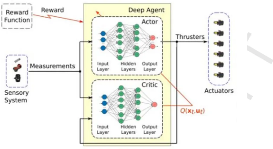
3.1. Deep RL actor-critic for continuous control
To solve the continuous control problem we employ an actor-critic model-free RL method based on the deterministic gradient theorem (Eq. (11)). In this architecture, the actor is an action selection policy that maps continuous states to continuous actions in a deterministic way and the critic is a state-value function mapping states to expected cumulative reward. However, in continuous control problems the actor and critic cannot be learned directly with the standard table-based Q-learning algorithm (Section 2) therefore function approximators are required.
In our formulation, we use a deterministic policy (as in Section 2.2) to approximate the actor behavior, ~ , with parameters that are updated periodically using a recursive rule as in Eq. (12). Therefore, the adaptability is achieved by means of the continuous update of the policy parameters based on the collected experience coming from the interactions between the robot and its environment. On the other hand, the critic is approximated as Q , ~Q , with a deep network Q ∙,∙ . Thus, this is a parametric function approximator, of the true state-action value function Q ∙,∙ , with all its parameters contained in a vector .
Due to the nature of the problem, the sensory system does not need to provide images to the control system and only low-level measurements of dynamic magnitudes are available at each time step . Therefore, we use an actor-critic architecture as in Fig. 2, where deep neural networks are used for the state-action value function and policy representation, respectively. As it can be seen we used deep fully connected neural networks of ReLU layers [50] without convolutional and pooling layers for these functions approximation. Due that the size of the input vector, given by the sensor measurements, it is dimensionally smaller than an average image frame, it is convenient to avoid the use of CNN. In this way, we drastically simplify the network architecture, the computational burden [66,67] and also we have a compatible function approximation for the critic representation [54,68].
In order to learn an optimal policy, we first must obtain an optimal critic function as in Eq. (5). To do this, in a continuous domain, we consider a deep neural network as a function approximator parameterized by and the optimal state-value function (critic function) can be found by minimizing the ordinary mean square error function, ∙ , defined as:
∑ Q , | (13)
where N represents a time horizon of N sampling times, dt. Then, the gradient of the mean square error function ∙ , is:
where are the target state-action values generated by other target deep network, Q, parameterized by , such that:
, Q , | (15)
where the target action is given by an actor target deep network, ̂, such that:
̂ | (16)
Then, the actor policy function represented by the deep network , is updated determining the critic parameters using the deterministic gradient theorem for optimizing the expected return (as in Eq. (11)). Thus, after the critic function is found it is used to update the actor function, being | and Q , | | , the deterministic policy gradient is given as in Eq. (17) and we use a stochastic optimization method [63] to obtain the optimal policy representation.
Q , | | ∙ |
(17)
The target networks parameters updates are made using the rules in Eq. (18) and (19) for the parameters of the actor and critic networks, respectively:
← 1 (18)
← 1 (19)
with ≪ 1. Note that two separated deep networks are used for generating the Q-learning targets and two for the actor approximations as in [52]. With the rules of Eq. (18) and (19) a weighted update of the weights of the targets networks is made instead of directly copying the weights, as is done in direct applications, which have been proven to be unstable in the learning phase. In this way, the networks parameters change slower than in direct applications improving the stability of the learning process [53].
Figure 2 3.2. Goa We seek operative co formulating As it can be The main fu level contro different op robot and it The syst robot sensor given for th generated b will be give information between th instantaneou and the fixe agent abou information As can b , , involves rea for a succe 2. Actor-criti al-oriented a k the adaptive onditions. T g a goal-orien e seen, a goa function of th olled variabl perative cond t allows a bro tem dynamic ry system, w he controlled by the goal-o en to the agen n provided b e current an us error vect ed set points ut the perfor n about the co be seen in Fi . An adily known essful low-l ic architectur actor-critic c e low-level c Thus, based o nted control al-oriented m his dynamic les of the A ditions of the oader explora c information which are com
d low-level v oriented mod nt by a modu by and nd the expe tor, , comp for such ma rmance of t ontrol system ig. 3, the dee advantage o n variables, y level control re using deep a control arch control system on the actor architecture module was in reference ge UV in a wi e underwater ation of the s n is the set o mbined in a v variables, co dule. Howev ule in a high , it is p cted dynami puted betwee agnitudes the autonom m behavior, s ep agent rece of perceiving yet they are i l. In additio p fully conne approximator hitecture m for the un r-critic archit as shown in ncorporated enerator is to de operative r vehicle. Th state space fo of measurem vector . Th ombined in v er, during a er hierarchy, possible to o ic behavior en the measu . Thus, mous control summarized eives inform g the system informative on, the state
ected neural rs. nderwater veh tecture of F n Fig. 3 in or with an emb o periodicall e range. In t his fact impl or the deep a ments of the c he current ta vector . real mission , such as a pa obtain a cha of the robo urements of t provides in l system its in the last ex mation summa m state ( ) enough to de e configurat network of R hicle to be ab ig. 2 we enh rder to achie bedded dyna ly change the this way, the ies totally di agent. controlled va arget specific . During trai n the request ath planning aracterization ot. This info the controlled nstantaneous elf. Also, th xecuted actio arized in the in this way escribe the a tion, , on ReLU layers ble to deal w hanced this eve a rich co amic referenc he set points e deep agen different beha ariables, obt cations are th ining the ve ted vel g module. Th n about the ormation is d variables s information he deep ag on, . e markovian y is the fact autonomous nly contains as function with different proposal by ontrol policy. ce generator. for the low-nt could face aviors of the ained by the he references ctor is locity vector hus, with the discrepancy given in an , at time , n to the deep ent receives system state that it only system state measurable t y . . -e e e s s r e y n , p s e y e e
information avoiding ex the deep lea
3.3. Dee Based o approach f developed a of our deep In line 1 each episod number o , … updating ra correlated O respectively Algorith data of a pr this reason, and ̂ are in In the R Thus, from Algorithm 1 episode the n coming fro xpensive com arning applic Figure ep RL algori on the prese for adaptive aiming to pre learning age of Algorithm de , the max of state trans , … suc ate for the Ornstein-Uhl y. This proce hm 1 was for re-trained po in line 2 and nitialized wit RL paradigm, m an algorith 1, each learn e random Or om common mputational t cations but ar e 3. Goal-orie ithm for AU ented goal-o low-level esent a comp ent for under
m 1, the inpu ximum size o sitions ch that ⊆ e deep targe lenbeck proc ess is incorpo rmulated to licy represen d in line 4, th th the same p , the low-lev hmic point o ning episode rnstein-Uhlen sensors, wh treatments as re not, howev ented control UV low-level oriented acto control for putationally rwater vehicl uts are the m of the replay
, , , which w et networks
ess noise wi orated for exp
learn a cont nted in the de here are both
parameteriza vel control pr of view, each
is carried ou nbeck stocha
hich are wide s in video im ver, mainly a l architecture l control or-critic arch AUVs. The feasible vers le low-level c maximum num y buffer , to be ta will be used parameters, ith scale fact ploration pur trol task from
eep network h options: to ation of Qan roblem of an h training ep ut in the loop astic process ely used in t mages which applied in the e based on ac hitecture, fo erefore, an sion. Thus, A control. mber of train , the minimu aken from th for minibatc the reward or and me rposes (line m scratch bu ks Q ∙,∙ | , initialize or nd , i.e. n AUV can b pisode is p from line 5 s is initialize the field of u are widely u e underwater ctor-critic arc ollowing we algorithmic Algorithm 1 ning episode um size of th e replay buf ch training, d function
ean and varia 11). ut it also can ∙ | and i load. In line and be seen as a defined alon to line 33. A ed (line 6), i underwater a used as inpu r domain. chitecture. develop ou representat outlines the es , the tim he replay buf ffer to def the discount ∙ and the ance paramet n continue le in a replay b 3 the target . continuous ng a time ho At the begin in order to c applications, ut in most of ur deep RL tion will be pseudocode me horizon of ffer , the fine a subset t rate , the e temporally ters and , earning from buffer . For networks, Q control task. orizon . In nning of each carry out the , f L e e f e t e y , m r Q . n h e
environment exploration and the dynamic variables of the system are obtained from the sensory system (line 7) to set the initial system state (line 8).
Into the inner loop from line 9 to 31 the core of the deep RL low-level AUV control algorithm is performed. Keeping in mind that our proposal is developed to be applied on a real robot we must keep a fixed sample time, . Then, the loop execution time must strictly be as long as a sampling time, , to satisfy the hardware constrains imposed by the technological the system. Thus, to achieve this requirement we use a timer to manage the execution time and guarantying a sample time . So, in line 10, we initialize a timer which waits a time lapse to continue with the execution of the Algorithm 1 in line 27. Note that must be long enough to allow the execution of the commands from line 11 to 26. Using the current actor control policy a control action is determined (line 11) and it is immediately sent to the actuators of the underwater vehicle (line 12).
Aiming to improve the stability of the learning process and to make an efficient use of the computational resources, we implement batch learning [69] using an experience replay buffer which can reach a maximum size . Thus, in the experience is stored in the form of transitions , such that
, … , . In this way, after each interaction step, the actor and critic are updated based on the experience stored in a replay buffer . To do this, if the buffer has stored at least transitions (i.e. condition of line 13 is true), a random minibatch of experimented transitions is sampled from (line 14). Then, with this subset of previous experience, in the inner loop from line 15 to 18 the state-action value targets ( ) are computed, which are necessary to obtain the critic parameterization , by miniminzing the loss function (Eq.13), and to obtain the actor parameterization . In this way, the actor and critic deep networks are parameterized as ∙ | and Q ∙ | (line 19-20). In line 21-22 the parameters of the target networks, ̂ ∙ | and ∙ | , are updated.
As was said, we use a replay buffer to store the experience thus when the buffer reaches its allowable maximum size we simply remove the oldest stored experience (line 24-26). Thus, with the dynamic measurements obtained from the sensory system the transition state representation is made (line 28). Then, with the transition state the instantaneous reward signal is computed using the reward function, i.e. (line 29). Next, with this information, the experimented transition , , , is incorporated into the buffer (line 30).
Finally, the outputs of the algorithm (line 34) are the low-level control policy, synthetized in the deep network ∙ | , the critic function summarized in the deep network Q ∙,∙ | and the buffer replay .
Algorithm 1. Deep RL algorithm for AUV low-level control 1. Inputs: , , , , , , , ∙, , ,
2. Randomly initialize/load critic network Q ∙,∙ | and actor network ∙ | with weights and , respectively
3. Initialize target networks and ̂ with weights and 4. Initialize /load replay buffer
5. For 1 to do
6. Initialize a random process , , for action exploration
7. Get AUV dynamic measurements from sensory system
8. Set initial state
9. For 1 to do
10. Initialize the
11. Select action | according to the current policy and exploration noise
12. Execute action over the system
13. If | | > then
14. Sample a random minibatch of transitions from , such that , … , … ⊆
15. For 1 to
16. With the target actor function ̂ ∙ | obtain ̂ | (Eq.(16))
17. Set the state-action value target Q , | (Eq.(15))
18. End
19. Obtain the critic parameterization minimizing the loss function (Eq.(13))
20. Obtain the actor policy parameterization using the deterministic policy gradient (Eq.(17))
21. Update the actor target network parameterization ← 1
22. Update the critic target network parameterization ← 1
23. End
24. If | | then
25. Remove the oldest ∗∈ from the replay buffer , i.e. ∗
26. End
27. Wait until is over
28. Get AUV dynamic measurements from sensory system and set the transition state
29. Observe the reward , i.e. )
30. Store the transition , , , in
31. End
32. Reset time, i.e. 1
33. End
4. AUV control experiments and results discussion
4.1. Experimental setupIn order to test our proposal the underwater vehicle Nessie VII (Fig. 4) developed by the Heriot-Watt University was used [70]. Briefly, this robot has six thrusters, indicated as T1 to T6 in Fig. 4, allowing for a five degree of freedom control (surge, heave, sway, pitch and yaw) and it is equipped with a DVL and an IMU to measure the linear and angular velocities. This underwater vehicle serves as an excellent platform for testing and development of underwater applications and it has already been used in various research articles as an experimental platform [18,45,46,71].
During the experiments the robot interacted with an external computer using ROS (Robot Operating System), exchanging messages in a network, with a sampling time 0.1 seconds. In this way, the on-board computer managed the sensory and navigation systems, while the external computer held the deep RL controller. The underwater vehicle is controlled by setting a vector , , , , , ), where
, … are the thrusters commands, at time , for the thruster 1, 2, … 6, respectively. These commands are determined by a control policy, synthetized in the actor deep neural network ∙ | (Algorithm 1).
In our deep RL problem formulation we define the markovian system state at time , using the observable state variables given by the instantaneous measurements from the robot sensors, as
, , , , , . The magnitudes , , and , , are the linear and angular velocities with respect to the axes , and , given by the DVL and IMU, respectively. Analogously, , , and , , are the linear and angular accelerations with respect to the axes , and , respectively. While is the vector of the commands executed in the previous time step 1 and is the instantaneous velocity error computed between the velocities at time and the fixed set points.
We seek to minimize the deviations of the controlled dynamic variables from their references whilst also trying to minimize the thruster use, to reduce overall energy consumption and sudden variations of the controlled signals. Note that in order to accomplish this we propose an appropriate reward function as in Eq.(20). In this way, the immediate reward, , is given by an evaluation of the effects the executed action ( ) had in the state of the system. This evaluation consists of three different terms:
λ exp Λ ∑ | | || : || (20)
where the first term evaluates the square error between the controlled dynamic variables ( ) and their references ( ) with Λ diag ℓ , ℓ , … , ℓ and ℓ , 1, … , , being the characteristic length-scales, the second term weights the thruster usage and the last term penalizes sudden changes in thrusters commands by computing the norm between the current action ( ) and the moving average of past taken actions ( : ). The mean : is backward computed using a slide windows of length . The parameters λ,
and are controlled v constrain th can be clea controlled d control poli maximized Figu scale factor variables fro he reward ma arly seen tha
dynamic var icy ( ) shoul instead of m ure 4. The au a rs ∈ 0, 1 . N m their refer agnitude to a at as the valu iables and c ld generate a maximizing ea utonomous u a) Experimen
Note that the rence but sa avoid numer ue of a decr onsequently a sequence of ach immedia underwater v ntal platform e first term aturates for s rical instabil reases, the r the control f actions , ate reward in (a) (b) vehicle, Ness University. m and facilitie of Eq.(20), p significant de ity in the lea reward funct task is more ,…, , … n Eq.(20). ie VII, desig es; b) AUV r penalizes for eviations. In arning proce tion spans a e challenging … such that t
ned and buil reference sys r great devia n this manner ess. Observin smaller inte ng. Note that the cumulati lt at the Heri stem. ations of the r, we aim to ng Eq.(20) it erval for the t the optimal ive reward is ot-Watt e o t e l s
4.2. Simulation results
The implementation of the Algorithm 1 was done in Python using Tensorflow2, a machine learning library with specially developed tools for deep learning applications. Hereinafter, as was mentioned in Section 3.1, for the policy network we used a deep fully connected neural network with an input layer of size 21, three hidden layers using ReLU activation functions, of size 600, 400 and 300, and one output layer of size 6, with sigmoid activation function, giving a total of 375056 free parameters. The state-action value function uses a similar deep neural network structure, with the difference that the state vector is fed to the input layer, and the action vector is fed to the first hidden layer. Moreover, before we begin describing the trials, we must mention that for both the simulated experiments and the wet experiments (presented in Section 4.3) in all trials we fix 500 episodes of length 700 time steps with sampling time of 0.1 seconds. The minimum and maximum size for the replay buffer were set in 100 and 200000 elements. The number of state transitions for the minibatch sampling was fixed as 60. We use a discount rate 0.99 and the updating rate for the deep target networks parameters is 0.001.
First, to illustrate the significance of each term for the reward function (Eq.(20)) we design a series of experiments which are shown in Fig. 5. Note that the simulated results3 showed in Fig. 5 were performed under the same training conditions for the different configurations of the reward function. The immediate reward is computed according to Eq. (20) with 1 and Λ diag 1,0.75,0.75,0.25,1, with a given set point for the controlled variables, , , , , and the action vectors , ,…, with 100.
Fig. 5a shows the results for a simple reward function where only the deviations of the controlled dynamic variables from their references are taken into account, i.e. 0, 0, 0. As it can be seen, Algorithm 1 finds a policy capable of achieving the target references for the dynamic variables,
, , , , 0.3 m/s, 0, 0, 0, 0 , however the thruster output patterns are too variable and aggressive to be applied in a real underwater vehicle. Fig. 5b depicts the results for a reward function that incorporates the second term, that is penalizing the usage of the thrusters, i.e. 0, 0 and 0 in Eq.(20). As it can be seen, Algorithm 1 finds a control policy capable of successfully control the AUV but the performance of the thruster outputs is still not suitable to be applied on real actuators. Following, we incorporate the third term to the reward function, i.e. we use the Eq. (20) with 0, 0 and 0, and again performed the same training experiment with Algorithm 1, obtaining the results showed in Fig. 5c. As it can be seen, the improvements in the results are clearly noticeable which validates the use of a reward function like the one presented in Eq.(20). Therefore, in the following experiments (simulated and real) we will adopt a reward function parameterized as the experiment of Fig. 5c, i.e. with 1, 0.75, 0.1,
0.4 and Λ diag 1,0.75,0.75,0.25,1 .
2 For further details refer to the web site https://www.tensorflow.org/. 3 For simulation we use the Nessie simulator [70].
a) R function In order level contro point was f this case, th despite the s Figure 5 Results for a r of Eq. (20) w to test the a olled variable fixed as he Algorithm
set point bee
5. Comparati reward funct with 0.7 algorithm ca es was chang 0.3,0.2, m 1 successfu en suddenly c ive examples tion of Eq. (2 5, 0.1 an 0.75 apability, we ged during a ,0.2,0,0 and ully controls changed to a (a) (b) (c) s for differen 20) with and 0; c) , 0.1 and carried out a trial. Fig. 6 d after 100 s the system, a considerably nt structures 0.75 and ) Results for d 0.4. an experime 6 shows the seconds was driving it rap y different o
for the rewar 0; b) a reward fun ent where th results for a changed to pidly toward perating regi rd function. Results for a nction of Eq. he reference a trial were th 0.5 ds the specifi ion. a reward (20) with
for the low-he initial set 5,0,0,0,0 . In ied reference -t n e
Figure 6. S in refere In order well-known 0.3,0.2,0.2 overshoot (o Figure Followin reference w operation. I due to the h exhibits a p task. The un major barrie control strat without pro imulations re nces from to make a p n PID contro 2,0,0 . Then, optimizing IT 7. Simulatio ng, Fig. 8 sh was changed In this case, i high nonline poor perform nknown dyn ers that cann tegy. Howev blems as cou esults of a tr 0.3 m performance oller used in , we find a TAE index) ns results for hows the re d from it is worth no arities, prope mance under namical mode not be effecti
ver, our prop uld be seen in
ial with a sud m/s, 0.2 m/s execut comparison n several pre set of gains and the obta
r a PID contr
sults for an 0.3,0.2 oting that the er of the dyn this requirem el and the co ively solved posed algorit n the results dden change s, 0.2 m/s, 0 tion of Algor of the Algo evious works s for a suitab ained simulat roller during analogous e ,0.2,0,0 to e dynamic b namics of an ment which oupling betw by one of th thm was abl shown in Fi e of the contr , 0 to rithm 1. orithm 1, we s. For this c ble performa tion results a g a trial with experiment t o behavior is no n underwater is a commo ween surge a he most pop e to successf g. 6. rolled variabl 0.5 m/s, compared o comparison e ance of the re shown in 0.3 to the show 0.5,0,0,0,0 ot the same f r vehicle. Cle n requiremen nd yaw moti ular control ful solve the
les, due to a , 0, 0, 0, 0 d our algorithm example we PID control Fig. 7. 3 m/s, 0.2, 0 wed in Fig. 6 after 100 for both ope early, the PI nt during an ions of the A technique, a e same contr step change during the m against the set llers without .2, 0, 0 . 6, where the seconds of rative points ID controller n underwater AUV are the as is the PID rol challenge e t e f s r r e D e
Figure variables is 4.3. Wet In order underwater underwater gyroscope, As was but it can a networks Q training exp on-line, in t gives flexib demonstrate inevitable b Initially, dynamic sp possible val policy able neighborhoo The expe University. controlled t transversal 0.5 m/s velocities a forward/bac (heave). Al 8. Simulation given a step t experimen to test our p vehicle Nes robot is eq acceleromete explained in also continu Q ∙,∙ | , ∙ periments on the real veh bility, reduc es the capab behavioral ga , during the t ecifications lues by the d to manipula od of an ope eriments wit Due to the the linear vel axes (yaw a
0.5 m are constrai ckward speed lso note that
ns results for p from ntal results proposed dee ssie VII as quipped with ers, DVL, IM n Section 3.2 ue the learni | and in a n the simulato icle, improv ing costs an bility of the ap between th training phas ( ) for th dynamic refe ate the unde erating point. th the real ro physical co locities (surg and pitch, r m/s, 0.2 m ined as d (surge), t the angular r a PID contr 0.2 m/s, ep RL appro an experime h all the ne MU, depth m 2, Algorithm ng process replay buffe or and then, ving and ada nd operation proposed te he simulator se with the A he controlled erence gener erwater vehic obot were car nstrains imp ge, sway and
espectively). m/s 0 is the latera r movement roller during , 0, 0, 0, 0 to
oach for adap ental platfor ecessary ins meter, and oth 1 was form from data o er . So, by
in a followin apting the low nal risks by
echnique to and the real AUV simula variables ( rator module cle within an rried out in t posed by the d heave) and . Therefore, 0.2 m/s a (no pitch al speed to th around the g a trial where o ptive low-lev rm to carry struments fo hers). mulated so as of a pre-train taking advan ng training st w-level cont learning ini self-adapt, s robot in its e tor, in each t ) are rando (Fig. 3). In n operation the Ocean Sy e AUV and the rotationa the control and 0 m/s or yaw ve he left/right ( longitudina e the referen 0.2 m/s, 0, 0 vel control o out a numb or underwate to learn a c ned policy s ntage of this tep, the learn trol policy. T itially on th since it is c environment training epis mly chosen w this way, w range instea ystem Labor the experim al movement led linear v 0.2 m locities). N (sway) and l axis (roll,
nce for the co 0, 0, 0 after of an AUV, ber of experi er navigation control task f summarized fact, we firs ning procedu This operatio he simulator. capable to ov t.
sode the set p within a cert we seek to lea ad of doing ratory of the mental faciliti ts around its velocities are m/s and t Note that, is the vert ) of the ontrolled 30 seconds. we used the iments. This n (compass, from scratch in the deep st carried our ure continues onal scheme . Besides, it vercome the points of the tain range of arn a control so only in a Heriot-Watt ies, we only vertical and e limited to: the angular refers to tical velocity AUV is not e s , h p r s e t e e f l a t y d : r o y t
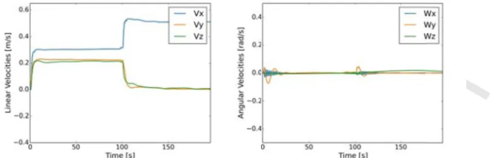
controlled. T The immed Λ diag 1 Using N 10 hours o training pha section we AUV so to the adaptive algorithm r simultaneou the vehicle different fro Figure 9 with a refe drives the v around its r also be seen real applica each thruste Figure 9. R Figure s, 0, 0, 0, 0 , useful, sinc different op linear backw Thus, at a ce diate reward 1,0.75,0.75,0 , , , Nessie’s simu f real intera ase using th show and d achieve the e features of runs, the le usly improvi changes sub om the backw 9 shows the erence vehicle to th reference val n that the an ations with un er. Results of a t 10 shows , in which th ce it allows t peration cond ward movem ertain time , is compute 0.25,1 , , and t ulator, we ran action) obtain e real robot, iscuss the ob fixed dynam f the propos arning proc ing the contr bstantially for
ward or later results of a
, , he reference
lues are dire ngular velocit nderwater ve training episo the results he low-level c to analyze th dition. Unlike ment. This op , the vector o ed according with a the action ve n Algorithm ning an init , fixing diffe btained resul mic specificat sed algorithm ess is activ rol policy. In r different op al behavior. training epi , , in just 10 s ectly associa ties measure ehicles [72]. ode for of a train control polic he capability e the previou eration settin of controlled g to Eq. (20 given set ectors , m 1 during 50 tial low-leve erent set poi lts of applyi tions. We se m to adapt th vely seeking n this sense, perating con sode carried 0.4 m/s, 0, seconds. No ated with the ements are no The right pa 0.4 m/s ning episode cy takes arou y of Algorith us case, the l ng is differen d variables is 0) with t point ,…, w 00 training e el control po ints for each ing Algorithm et different o he control p g to achieve it is also wo nditions, for e d out on the , 0, 0, 0 . As ote that the v
e noise of th oisier. Howe anel of Fig. 9
s, 0, 0, 0, 0 d e with und ten secon
hm 1 to ada learned contr nt to the prev defined as 1, 0.75 for the with 100 episodes (this olicy. Afterw h training ep m 1 for the perational co policy. It is w e the dynam orth mentioni example its f real experim it can be s variation of e measuring ever, this phe 9 shows the
during the exe
, , nds to reach t apt the low-l rol policy mu vious results , , 5, 0.1, controlled 0. s is equivale wards, we co pisode. In the low-level co onditions to worth noting mic specifica ing that the forward beha mental platfo seen, the co the controll g instruments enomenon is usage (in pe ecution of A , , the set point. level control ust drive the (Fig. 9) in th , , , . 0.4 and variables, ent to almost ontinued the e rest of the ontrol of the demonstrate g that as the ations while dynamics of avior is very orm (Fig. 4), ontrol policy led variables s and, it can s common in ercentage) of Algorithm 1. 0.4 m/ . This case is l policy to a e vehicle in a he sense that . d , t e e e e e e f y , y s n n f / s a a t
the forward for example may vary demonstrate Figure 10. In Fig. 1 heave veloc policy succ 4), therefore Figure 11. R A more movement ( directly gen composition a training ep the vehicle t
d and the bac e, the thruste according t es the ability
Results of a
11 the results city was set t essfully achi e their relativ Results of a t complex con (sway) is req nerate a pure n of the engi pisode with towards the ckward dynam ers are not sy
to the direc y of the propo
training epis
s of an episo to 0.18 m/s, ieves the spe ve higher usa training episo ntrol task wa quested. It s e lateral displ nes to achiev sway velocit specified set mics exhibite ymmetrically ction of rot osed Algorith sode for ode with a p i.e. ecification. T age can be ea ode for as imposed b should be no lacement, th ve this pure l ty 0.1 t point in alm ed a differen y located in t tation, amon hm 1 to adap 0.4 m 1. ositive heav 0,0, 0.18m/ The thrusters asily underst 0,0, 0.18 by setting oted that the hat is, the con lateral displa 1. As it can b most 16 secon nt behavior. T the AUV bo ng others. I pt itself while m/s, 0, 0, 0, 0 e velocity as /s, 0, 0 . As s 5 and 6 are tood as it is s 8 m/s, 0, 0 0, 0 thrusters of ntrol system acement. Fig be seen, the nds. This differen dy, the force In summary e facing a dif during the s set point ar it can be see e placed vert showed in the during the ex 0.1 m/s, 0, 0, f the AUV a must determ ure 12 show control polic
nce has mult e made by th y, this exam
fferent situat
execution of
re shown. Th en, the low-l rtically in the e right panel
xecution of A
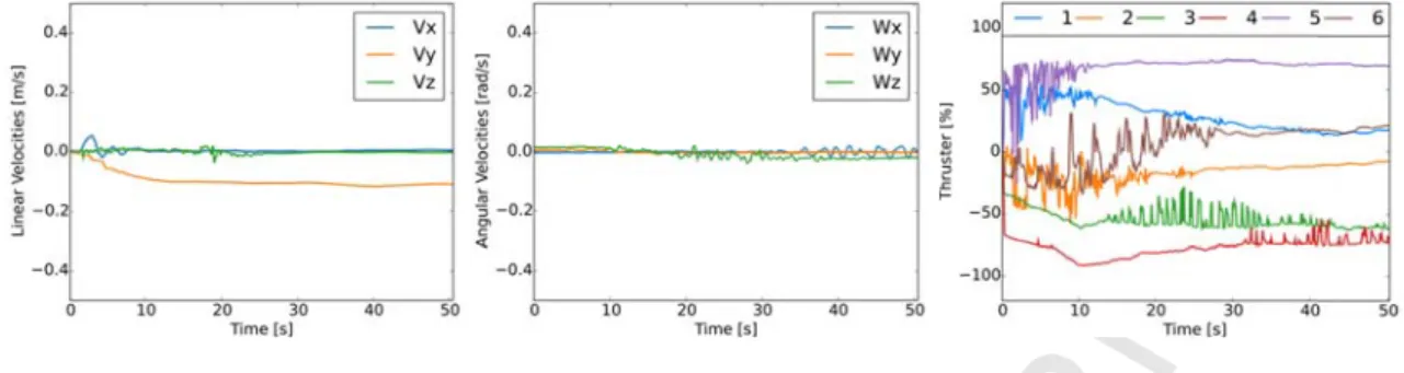
, 0 , where a are not arran mine the nece ws the obtaine cy can succe iple reasons, he propellers mple further tion. f Algorithm he requested level control e AUV (Fig. l of Fig. 11. Algorithm 1. a pure lateral ged so as to essary thrust ed results for ssfully drive , s r d l . l o t r e
Figure 12. In order 0.2m/s, combined m and 0.1 m/s level contro seconds. Figure 13 As we c present. For reference ve used. Howe but, on the c a positive li a dynamic s developmen Results of a to make the 0.1 m/s, 0 movement of s, respectivel ol policy was 3. Results of could see al r example, if elocity, a pr ever, not only
contrary, a m inear velocity system with nt of this kin training epis e control task , 0, 0 . With f the AUV w ly. Figure 13 s successfully a training ep
ong the pres f we look at riori, we wo y the two fo more complex y (forward v a complex d of adaptive sode for k even harde h this reques with a simult 3 shows the o y adapted by pisode for sented result the case sho uld intuitive rward facing x thrusters ou elocity) and couple dyna e control tech 0, 0.1 1. er, during a sted referenc taneous back obtained resu y Algorithm 0.2m Algorithm 1 ts, the unde wed in Fig. ely expect th g thrusters m utput schem the others nu amics hard to hniques. 1 m/s, 0, 0, 0 training epis ce the contr kward and lat ults for this e 1 achieving
m/s, 0.1 m .
rlying nonli 9, where the hat only the t must be used e was needed ull. This fact o be modele
during the
sode the set rol policy m teral motion episode. In t the requeste m/s, 0, 0, 0 d nearities of e AUV must two forward to achieve a d to satisfy a t shows that d and contro execution of point was se must achieve n with a spee this case, aga ed velocities during the ex the AUV d follow a sim d facing thru a positive sur a dynamic re an underwat olled, which f Algorithm et as e a complex ed of 0.2 m/s ain, the low-in almost 18 xecution of dynamics are mple forward sters will be rge velocity, ference with ter vehicle is justifies the x s -8 e d e , h s e
5. Final Remarks
In this work an adaptive controller based on the deep RL framework was proposed for low-level control of an AUV. The proposed algorithm uses only the low-level data provided by the on-board sensors of the vehicle to make the decisions needed for successfully solving the continuous control task. Moreover, unlike classic control theory, which requires a model of the system, or fuzzy control strategies, that requires prior expert knowledge, the proposed algorithm carries out a specialization process with minimum prior knowledge. Effectively, using only the input parameters the deep agent is able to learn a successful control strategy. Note that the reward function design is an important part for the implementation of deep RL methods in autonomous systems. In this sense, in this work a detailed reward function analysis and development was carried out to successfully satisfy the physical and operative constrains required by the AUV such as restraining the actuators sudden changes, optimization of the energy consumptions and others. In addition, an actor-critic goal-oriented architecture was developed to aid the deep agent to achieve a more generalized policy and therefore solve a bigger range of dynamic problems.
It is important to note that many previous approaches, based on deep RL framework, have used images as inputs for the state representation in order to learn a policy able to solve the control tasks. However, this type of representations are not straightforward for underwater applications where underwater images are not clear and require artificial lightning sources, which in turn increases the energy consumption of the vehicle diminishing the available mission time. In addition, the computational requirement for such an application raises the need for higher computational capability on board of the AUV, therefore increasing the energy consumption even further. Moreover, an additional image processing is needed to obtain the immediate reward from a sequence of images, which is not a trivial problem in real-time applications. In contrast, our proposed adaptive low-level control algorithm based on deep RL framework only uses a low-level representation of the system state, based on the measures of dynamic magnitudes (linear and angular velocities), therefore higher computational costs are avoided.
The articles found in the literature with similar features to the present work, were only tested in simulation where the characterization of the systems and its environments were always available. Instead of this, our work contributes with valuable experimental results which demonstrate the capability and the successful performance of the proposed approach for AUV low-level control. During the experiments we worked with Nessie, an AUV developed at Heriot-Watt University, obtaining satisfactory results which demonstrate the feasibility of the proposed control approach to be implemented as an adaptive low-level control strategy of AUVs.
Previous works on AUVs, controlled only a limited amount of degrees of freedom, or utilized different discretization schemes to be able to control the AUV. However, this article showed that it was possible to control the six degrees-of-freedom of a real underwater vehicle by directly sending the low-level commands to the thrusters. In this sense, we think that this work is a relevant contribution for the field of autonomous underwater robotics opening a new area of research by means of including deep RL for autonomous control
formulations of AUVs. However, further research is necessary to improve the general autonomy of the robots. For example, it would be interesting to consider the possibility of enhancing our proposal by adding prior expert knowledge or combining our proposal with other low-level control techniques. Moreover, it would be also possible to include safety constraints for the training phase, or utilizing a more complex supervisor layer. It would also be interesting to test the proposed approach in other types of mobile robots due that our proposal is of a general nature and it is not only restricted to AUVs.
Our proposed approach uses recently developed ideas coming from the emergent branch of deep learning in the artificial intelligence community. Nowadays, deep RL is at an early stage and in this paper we have contributed with real evidence for its application in robot adaptive low-level control, particularly, for AUV applications. However, there are open issues that deserve attention in the immediate future. For example, about how the efficiency of the learning process is affected by the different configurations of the adopted deep networks architectures, for functions approximation, is a not trivial issue that deserves a thorough discussion and quantitative analysis that could be the subject for future research papers. Finally, for this and other issues, there are several open issues for future research regarding deep reinforcement learning as a powerful tool for real autonomous developments in underwater robotics.
Acknowledgements
We gratefully acknowledge the support of NVIDIA Corporation with the donation of the Titan X Pascal GPU used for this research. The authors would like to especially thank Len McLean, the technician of the Heriott-Watt University, for all the help during trials, and the people of the Ocean System Laboratory for hosting this research. Particularly, we thank UNCPBA and CONICET for the financial support of Ignacio Carlucho at the Ocean System Laboratory.
References
[1] M. Chyba, Autonomous underwater vehicles, Ocean Eng. 36 (2009) 1. doi:10.1016/j.oceaneng.2008.12.005.
[2] A. Rozenfeld, G. Acosta, A. Sousa, H. Curti, O. Calvo, A guidance and control system proposal for autonomous pipeline inspections, Trans. Syst. Signals Devices. 5 (2010) 5–27.
[3] K. Alam, T. Ray, S.G. Anavatti, Design and construction of an autonomous underwater vehicle, Neurocomputing. 142 (2014) 16–29. doi:10.1016/j.neucom.2013.12.055.
[4] M. Knudson, K. Tumer, Adaptive navigation for autonomous robots, Rob. Auton. Syst. 59 (2011) 410–420. doi:10.1016/j.robot.2011.02.004.
[5] S.A. Gafurov, E. V. Klochkov, Autonomous Unmanned Underwater Vehicles Development Tendencies, Procedia Eng. 106 (2015) 141–148. doi:10.1016/j.proeng.2015.06.017.
[6] B. Jalving, The NDRE-AUV flight control system, IEEE J. Ocean. Eng. 19 (1994) 497–501. doi:10.1109/48.338385. [7] T.I. Fossen, O.-E. Fjellstad, Robust Adaptive Control of Underwater Vehicles: A Comparative Study, IFAC Proc. Vol. 28
(1995) 66–74. doi:10.1016/S1474-6670(17)51653-5.
[8] F. Valenciaga, P.F. Puleston, O. Calvo, G.G. Acosta, Trajectory Tracking of the Cormoran AUV Based on a PI-MIMO Approach, in: Ocean. 2007 - Eur., IEEE, 2007: pp. 1–6. doi:10.1109/OCEANSE.2007.4302301.