ODEs by means of high-order Taylor methods
`
Angel Jorba
(1)and Maorong Zou
(2)27th January 2004
(1) Departament de Matem`atica Aplicada i An`alisi, Universitat de Barcelona, Gran Via 585, 08007 Barcelona, Spain. E-mail: [email protected]
(2) Department of Mathematics, The University of Texas at Austin, Austin, TX 78712-1082, USA. E-mail: [email protected]
To the memory of William F. Schelter
Abstract
This paper revisits the Taylor method for the numerical integration of initial value problems of Ordinary Differential Equations (ODEs). The main goal is to show that the Taylor method can be competitive, both in speed and accuracy, with the standard methods. To this end, we present a computer program that outputs an specific numerical integrator for a given set of ODEs. The generated code includes adaptive selection of order and step size at run time. The package provides support for several extended precision arithmetics, including user-defined types.
The paper discusses the performance of the resulting integrator in some ex-amples, showing that it is a very competitive method in many situations. This is specially true for integrations that require extended precision arithmetic. The main drawback is that the Taylor method is an explicit method, so it has all the limitations of these kind of schemes. For instance, it is not suitable for stiff systems.
Contents
1 Introduction 3
2 A short summary on automatic differentiation 5
2.1 Rules of automatic differentiation . . . 6
2.2 An example: The Van der Pol equation . . . 7
3 Degree and step size control 8 3.1 The effect of roundoff errors . . . 9
3.1.1 On the Taylor polynomial . . . 9
3.1.2 On the normalized derivatives . . . 9
3.2 On the optimal selections . . . 10
3.3 Estimations of order and step size . . . 12
3.4 High accuracy computations . . . 13
4 Software implementation 14 4.1 The input file . . . 14
4.2 The jet of normalized derivatives . . . 14
4.3 Order and step size control . . . 15
4.3.1 First step size control . . . 15
4.3.2 Second step size control . . . 15
4.3.3 User defined step size control . . . 16
4.4 Extended arithmetic . . . 16
4.5 Using the package . . . 17
5 Some tests and comparisons 19 5.1 The Restricted Three-Body Problem . . . 19
5.1.1 Local error . . . 20
5.1.2 Global error . . . 20
5.1.3 On the influence of the underlying arithmetic . . . 23
5.1.4 Extended precision calculations . . . 23
5.2 Speed . . . 25
5.2.1 A simple comparison with ADOL-C . . . 27
6 Conclusions 29
1
Introduction
Let us consider the following problem: find a smooth function x: [a, b]→Rm such that
x0(t) = f(t, x(t)),
x(a) = x0, (1)
where f : [a, b]×Ω ⊂ R×Rm → Rm is a smooth function, Ω = Ω and◦ m ≥ 1. There
is a classical result of the theory of ODE that ensures the existence and uniqueness of a functionx(t), defined on [a, b0]⊂[a, b], satisfying (1). However, the effective computation
of such a function is a much more difficult question.
The search of good numerical methods for (1) is one of the classical problems in numerical analysis. The usual procedures are based on approximating the values x(t) on a suitable mesh of values of t. For the moment, and to simplify the presentation, we will use an equispaced mesh and we will assume that x(t) is defined on the whole interval [a, b]. Therefore, if M ∈N, we define
h= b−a
M , tm =a+mh, 0≤m≤M.
The problem now is to find approximations xm to the exact values x(tm). The
compu-tation of these approximations xm is usually performed recurrently from the (previously
computed) values x0, . . . , xm−1. Each step of this recurrence is known as a time step, and
its computer implementation is also called a time-stepper.
In this paper we will revisit one of the oldest numerical procedures for the numerical integration of ODEs: the Taylor method. For simplicity, we will assume that the function
f is analytic for (t, x)∈[a, b]×Ω. The idea of the method is very simple: given the initial condition x(tm) = xm, the value x(tm+1) is approximated from the Taylor series of x(t)
att =tm. The algorithm is then,
x0 = x(a), xm+1 = xm+x0(tm)h+ x00(t m) 2! h 2+· · ·+x(p)(tm) p! h p , m = 0, . . . , M −1. (2)
We refer to [HNW00] for a discussion of the basic properties of the method. One of the key points for a practical implementation is the effective computation of the values of the derivatives x(j)(t
m). A first procedure to obtain them is to differentiate the first equation
in (1) w.r.t. t, at the point t=tm. Hence,
x0(tm) =f(tm, x(tm)), x00(tm) = ft(tm, x(tm)) +fx(tm, x(tm))x0(tm),
and so on. Therefore, the first step to apply this method is, for a givenf, to compute these derivatives up to a suitable order. Then, for each step of the integration (see (2)), we have to evaluate these expressions to obtain the coefficients of the power series ofx(t) att =tm.
Usually, these expressions will be very cumbersome, so it will take a significant amount of time to evaluate them numerically. This, jointly with the initial effort to compute the derivatives of f, is the main drawback of this approach for the Taylor method.
This difficulty can be overcomed by using the so-called automatic differentiation ([BKSF59], [Wen64], [Moo66], [Ral81], [GC91], [BCCG92], [BBCG96], [Gri00]). This is a procedure that allows for a fast computation of the derivatives of a given function, up to arbitrarily high orders. As far as we know, these ideas were first used in Celestial Mechanics problems ([Ste56], [Ste57]; see also [Bro71]).
An inconvenience of this method is that the function f has to belong to a special class; fortunately, this class is large enough to contain the functions that appear in many applications. We also note that the program that computes these derivatives by automatic differentiation has to be specifically coded for each functionf. This coding can be either done by a human (see, for instance, [Bro71] for an example with theN-body problem) or by another program (see [BKSF59, Gib60, CC94] for general-purpose computer programs). An alternative procedure to apply the Taylor method can be found in [SV87] and [IS90]. One of the goals of this work is to present a software that, given a functionf (belonging to a suitable class), generates a complete time-stepper based on Taylor method. The generated code is ANSI C, but we also provide a Fortran 77 wrapper for the main call to the time-stepper.
A software package that performs a similar task is ATOMFT (written by Y.F. Chang) that can be freely downloaded from the Internet (to get a copy you can visit, for in-stance, http://www.eng.mu.edu/corlissg/FtpStuff/Atom3_11/ and retrieve the file atom3_11.tar.Z). ATOMFT is written in Fortran 77 and it reads Fortran-like state-ments of the system of ODEs and writes a Fortran 77 program that is run to numerically solve the system using Taylor series.
One of the nicest characteristics of Taylor method is the possibility of using interval arithmetic to derive bounds for the total error of the numerical integration. These ideas have been used in ATOMFT to compute a step size that guarantees a prescribed accuracy, but using the standard floating point of the computer instead of interval arithmetic. We also want to note that the step size selections in “usual” numerical integrators (Runge-Kutta, Adams-Bashford, etc.) are based on the asymptotic behaviour of the error, and they do not provide true bounds for the truncation error of the method. On the other hand, the derivation of the time step in ATOMFT is a substantial part of the computing time, while an estimation based on the asymptotic behaviour of the error is usually much faster.
Here, we have implemented a step size control based on an asympotic estimate of the error. The main reason for this selection is that we want to compete against the “usual” numerical integrators – which use similar step size control techniques. Moreover, as we will see later, our software allows the user to plug in its own step size control, so it is not difficult to implement different strategies.
For an efficient numerical integration, we need some knowledge of the order p∈N up to which the derivatives have to be computed, and an estimate of the step size h, in order to have a truncation error of the order of a given threshold value ε. We note that, as we have to select the value of two parameters (p and h), we can ask for a second condition besides the size of the truncation error. Here we have chosen to minimize the number of operations needed to advance the independent variable t in one unit ([Sim01]). We have also coded the algorithms to do these tasks so that the output of the program is, in fact, a
complete numerical integrator –with automatic order and step size control– for the initial value problem (1).
We have tested this Taylor integrator against some well-known integration methods. The results show that Taylor method is a very competitive method to integrate with the standard double precision arithmetic of the computer. However, the main motivation for writing this software is to address the need of highly accurate computations in some problems of Dynamical Systems and Mechanics (see, for instance, [MS99], [SV01] and [Sim]). Methods whose order is not very high (less than, say, 12) can be extremely slow for computations requiring extended precision arithmetic. This is one of the strong points of the software presented here: note that Taylor method does not need to reduce the step size to increase accuracy; it can simply increase the order (see Section 3.4). As we will see, this allows to greatly reduce the total number of arithmetic operations during the numerical integration.
As any explicit scheme, the Taylor method is not suitable for stiff equations because, in this case, the errors can grow too fast. However, there are modifications of the Taylor method to deal with these situations ([Bar80], [JZ85], [KC92] and [CGH+97]). These
modifications have not been considered in our software.
In the paper we present the main details of our implementation. We have tried to produce an efficient package, in the sense that the produced Taylor integrator be as fast as possible. Moreover, we have also included support for multiple precision arithmetic. We have done several test to compare the efficiency and accuracy of the generated Taylor routine against other numerical integrators.
There are several papers that focus on computer implementations of the Taylor method in different contexts; see, for instance, [BWZ70], [CC82], [CC94] and [Hoe01]. A good survey is [NJC99] (see also [Cor95]).
The package has been released under the GNU Public License, so anybody with In-ternet access is free to get it and to redistribute it. To obtain a copy, yo can visit the URLs
http://www.ma.utexas.edu/~mzou/taylor/ (US) http://www.maia.ub.es/~angel/taylor/ (Europe)
We note that the actual version of the package is written to run under the GNU/Linux operating system. We do not expect major problems to run it under any version of Unix, but we do not plan to write ports for other operating systems.
The paper has been split as follows: Section 2 contains a survey about automatic differentiation, Section 3 is devoted to the selection of step size and truncation degree, Section 4 gives some details about the software and Section 5 provides some tests and comparisons.
2
A short summary on automatic differentiation
Before starting with the discussion of the package, we will summarise the main rules of automatic differentiation.
Automatic differentiation is a recursive procedure to compute the value of the deriva-tives of certain functions at a given point (see [Moo66, Ral81]). The considered functions
are those that can be obtained by sum, product, quotient, and composition of elemen-tary functions (elemenelemen-tary functions include polynomials, trigonometric functions, real powers, exponentials and logarithms).
2.1
Rules of automatic differentiation
To simplify the discussion let us introduce the following notation: if a :t ∈I ⊂ R 7→ R denotes a smooth function, we call its normalized n-th derivative to the value
a[n](t) = 1
n!a
(n)(t). (3)
where a(n)(t) denotes the n-th derivative of a w.r.t. t. In what follows, we will focus on
the computation of the values a[n](t).
Assume now that a(t) = F(b(t), c(t)) and that we know the values b[j](t) and c[j](t),
j = 0, . . . , n, for a given t. The next proposition gives the n-th derivative of a at t for some functionsF.
Proposition 2.1 If the functions b and care of class Cn, and α ∈R\ {0}, we have
1. If a(t) =b(t)±c(t), then a[n](t) =b[n](t)±c[n](t). 2. If a(t) =b(t)c(t), then a[n](t) = n X j=0 b[n−j](t)c[j](t). 3. If a(t) = b(t) c(t), then a [n](t) = 1 c[0](t) " b[n](t)− n X j=1 c[j](t)a[n−j](t) # . 4. If a(t) =b(t)α, then a[n](t) = 1 nb[0](t) n−1 X j=0 (nα−j(α+ 1))b[n−j](t)a[j](t). 5. If a(t) =eb(t), then a[n](t) = 1 n n−1 X j=0 (n−j)a[j](t)b[n−j](t). 6. If a(t) = lnb(t), thena[n](t) = 1 b[0](t) " b[n](t)− 1 n n−1 X j=1 (n−j)b[j](t)a[n−j](t) # . 7. If a(t) = cosc(t) and b(t) = sinc(t), then
a[n](t) =−1 n n X j=1 jb[n−j](t)c[j](t), b[n](t) = 1 n n X j=1 ja[n−j](t)c[j](t).
Proof: These proofs can be found in the literature, so we only give some hints about them.
2. It follows from Leibniz’s formula: a[n](t) = 1 n!a (n)(t) = 1 n! n X j=0 n j b(n−j)(t)c(j)(t) = n X j=0 b[n−j](t)c[j](t). 3. Apply item 2 to a(t)c(t) =b(t).
4. Take logarithms and derivatives to obtaina0(t)b(t) =αa(t)b0(t). Use item 2 and (3).
5. Take logarithms and derivatives to obtain a0(t) =a(t)b0(t). Use item 2 and (3).
6. Take derivatives to obtain a0(t)b(t) =b0(t). Use item 2 and (3).
7. Take derivatives to obtaina0(t) =−b(t)c0(t) andb0(t) =a(t)c0(t). Use item 2 and (3).
Remark 2.1 It is possible to derive similar formulas for other functions, like inverse trigonometric functions.
Corollary 2.1 The number of arithmetic operations to evaluate the normalized deriva-tives of a function up to order n is O(n2).
Proof: The number of operations to obtain thej-th derivative once we know the previous ones isO(j). Hence, the total number of operations isPn
j=1O(j) = O(n2).
Although these methods only allow for the derivation of a reduced subset of the set of analytic functions, we note that they cover the situations found in many applications.
2.2
An example: The Van der Pol equation
These rules can be applied recursively so that we can obtain recursive formulas for the derivatives of a function described by combination of these basic functions. As an example, we can apply them to the Van der Pol equation,
x0 = y
y0 = (1−x2)y−x
.
To this end we decompose the right-hand side of these equations in a sequence of simple operations: u1 = x u2 = y u3 = u1u1 u4 = 1−u3 u5 = u4u2 u6 = u5−u1 x0 = u 2 y0 = u 6 (4)
Then, we can apply the formulas given in Proposition 2.1 (items 1 and 2) to each of the equations in (4) to derive recursive formulas foru[jn], j = 1, . . . ,6,
u[1n](t) = x[n](t), u[2n](t) = y[n](t), u[3n](t) = n X i=0 u[1n−i](t)u [i] 1 (t), u[4n](t) = −u[3n](t), u[5n](t) = n X i=0 u[4n−i](t)u[2i](t), u[6n](t) = u[5n](t)−u[1n](t), x[n+1](t) = 1 n+ 1u [n] 2 (t), y[n+1](t) = 1 n+ 1u [n] 6 (t). The factor 1
n+1 in the last two formulas comes from the definition given in equation (3).
Then, we can apply recursively these formulas forn = 0,1, . . ., up to a suitable degree p, to obtain the jet of normalized derivatives for the solution at a given point of the ODE. Note that is not necessary to select the value ofp in advance.
One of the tasks of the software we present is to read the system of ODEs, to decompose it into a sequence of basic operations, and to apply the formulas in Proposition 2.1 to this decomposition. This results in an ANSI C routine that, given an initial condition x0 and
a degree p, returns the jet of normalized derivatives of the solution at the pont x0 up to
degreep.
3
Degree and step size control
In this section we will discuss the sources of error of the Taylor method, and how to select the order p and step size h (see eq. (2) for the notation) to control both accuracy and efficiency.
First, note that the power expansion of the solution x(t) at t = tm can have very
different radius of convergence for differenttm, and that an efficient integration algorithm
must take this into account. This means that, at each step (i.e., for each m), we have to compute suitable values p=pm and h=hm.
Moreover, as we have two parameters (order and step size) to achieve a given level of accuracy, we can try to impose a second requirement: to minimise the total number of arithmetic operations to go fromt =a tot=b, so that the resulting method is as fast as possible.
3.1
The effect of roundoff errors
An extra source of error comes from the use of floating point arithmetic, and it mainly affects to the computation of the sequence of normalized derivatives and the evaluation of the Taylor polynomial.
3.1.1 On the Taylor polynomial
Before discussing the selection of order and step size, we want to note that different selec-tions ofp and h (with the same truncation error) can lead to very different propagation of roundoff errors in the evaluation of the Taylor polynomial.
As an example, consider the initial value problem
x00=−x, x(0) = 0, x0(0) = 1,
and assume we are interested in computing x(8π), by numerical integration of the ODE, with an error below 10−15. We know that the solution is x(t) = sin(t), so x(8π) = 0. The
Taylor series of the solutionx(t) at t= 0 is:
x(h) = ∞ X j=0 (−1)j h2 j+1 (2j+ 1)!. (5)
Due to the entire character of this function, we can think of using the step h = 8π (so only one step will be needed) combined with a sufficiently high order. It is not difficult to check that it is enough to sum the previous power series up toj = 95 to have a truncation error less than 10−15. Then, a straightforward application of Horner’s method with double
precision arithmetic gives x(8π)≈2.6965×10⁻⁷, which is unacceptable.
The source of the problem is that, in our case, the series (5) contains large terms that cancel out and lead to the loss of many significant digits when the sum is carried out with floating point arithmetic.
A solution for this problem is to use smaller values ofh, to avoid these cancellations. In fact, these cancellations cannot happen if we use a step size such that the terms in the series are decreasing in modulus. For instance, in this case we should useh= 1 (and then several integration steps to reach t = 8π). This phenomenon will be discussed again in Section 4.3.2.
3.1.2 On the normalized derivatives
Due to the use of floating point arithmetic, the computation of the derivatives is also affected by the roundoff. Moreover, the recurrent character of this computation implies that these errors can propagate such that higher derivatives will have, in principle, larger errors. Although a detailed study strongly depends on the vector field considered, here we will discuss this issue in an informal manner.
For instance, let us assume that we are making a single step of the Taylor method with order pan step size h, to achieve an accuracy ε. Let us write this step as
xm+1 = p−1 X j=0 x[j] mh j+x[p] mh p,
and let us focus on the last term x[mp]hp. Note that, if ε is small, the contribution of this
term to the total sum should be small. Therefore, this term (and, hence, x[mp]) does not
need a high relative accuracy because, roughly speaking, we do not need digits whose contribution goes below ε. Of course, we can apply this reasoning to all the normalized derivatives so that we can allow for an increasing error in x[mj] when j increases, without
affecting the global error.
This property results in a very good behaviour for the error propagation of the Taylor method.
3.2
On the optimal selections
Assume that, for a given time tm, the solution is at the point xm, and that we want to
compute the position of the trajectory for a new timetm+1 =tm+hm within a given error
ε. We will not assume that tm+1 is fixed in advance, so we have to determine not only
the degree of the Taylor expansion to be used but also the value hm.
So, let us denote by {x[mj](tm)}j the jet of normalized derivatives at tm of the solution
of (1) that satisfies xm(tm) =xm. Then, if h=t−tn is small enough, we have
xm(t) =
∞
X
j=0
x[mj](tm)hj.
Therefore, we want to select a sufficiently small value hm and a sufficiently large value p
such that the values
tm+1 ≡tm+hm, xm+1 ≡ p X j=0 x[mj](tm)hjm, satisfy kxm(tm+1)−xm+1k ≤ε,
and, moreover, we want the total number of operations of the numerical integration to be as small as possible. To determine such values, we need some assumptions on the analyticity properties of the solution x(t). The following result can be found in [Sim01].
Proposition 3.1 Assume that the function h7→x(tm+h)is analytic on a disk of radius
ρm, and that there exists a positive constant Mm such that
|x[j]
m| ≈
Mm
ρjm
Then, if the required accuracy ε tends to 0, the optimal value of h that minimizes the number of operations tends to
hm =
ρm
e2 ,
and the optimal order pm behaves like
pm =− 1 2ln ε Mm −1.
Remark 3.1 Note that the optimal step size does not depend on the level of accuracy. The optimal order is, in fact, the order that guarantees the required precision once the step size has been selected.
Proof: Although the proof can be found in [Sim01], we will include it here for the convenience of the reader.
The error introduced when cutting a Taylor series to a given degree p is of the order of the first neglected term,
E ≈Mm h ρ p+1 .
Hence, to obtain an error of order ε we have to select
h≈ρ ε Mm p+11 , (6)
On the other hand, the computational effort to obtain the jet of normalized derivatives up to order pis O(p2)≈c(p+ 1)2 (see Corollary 2.1). So, the (instantaneous) number of
floating point operations per unit of time is given, in order of magnitude, by
φ(p) = c(p+ 1) 2 ρm ε Mm p+11 ,
and, solving φ0(p) = 0, we obtain
p=−1 2ln ε Mm −1.
Finally, inserting this value of pin (6) we have h= ρ
e2.
There are strategies to use step sizes that are larger than the radius of convergence of the series (see [CC82]), but they only work for some singularities and require some computational effort (although this effort can pay off when the solution is close enough to one of the considered singularities). As it has been mentioned before, we have implemented a more straightforward algorithm based on Proposition 3.1.
3.3
Estimations of order and step size
The main drawback of Proposition 3.1 is that it requires information that we cannot obtain easily, like the radius of convergence of the Taylor series or the value of Mm. In
this section we will first describe, schematically, the numerical implementation and, then, we will give some comments on it.
Let us denote by εa and εr the absolute and relative tolerances for the error. The
method we propose uses only one of these two requirements: ifεrkxmk∞≤εawe will try to
control the absolute error usingεa; otherwise we will try to control the relative error using
εr. Note that, in any case, we are controlling the absolute error by max{εa, εrkxmk∞}.
First, we compute the order pm for the Taylor method as follows: we define εm as
εm = εa if εrkxmk∞≤εa, εr otherwise, (7) and then, pm = −1 2lnεm+ 1 . (8)
whered.estands for the ceiling function. If we compare with Proposition 3.1, we see that here the value Mm has been taken as 1 and that pm is two units larger. The reason for
these differences will be discussed later on.
To derive the step size, we will also distinguish the same two cases as before: if
εrkxmk∞≤εa, we define ρ(mj) = 1 kx[mj]k∞ !1j , 1≤j ≤p, (9) and, if εrkxmk∞> εa, we take ρ(j) m = kxmk kx[mj]k∞ !1j , 1≤j ≤p. (10)
In any case, we estimate the radius of convergence as the minimum of the last two terms,
ρm = min ρ(p−1) m , ρ( p) m , (11)
Hence, the estimated time step is
hm =
ρm
e2 . (12)
Now, it is natural to ask for the truncation error corresponding to order pm and step
hm, specially in the case Mm 6= 1.
Proposition 3.2 Assume that the hypotheses in Proposition 3.1 hold, and that Mm is
1. If εrkxmk∞ ≤εa, and pm and hm are defined as before, we have kx[pm−1] m h pm−1 m k∞≤εa, kx[mpm]h pm m k∞ ≤ εa e2. 2. If εrkxmk∞> εa, and pm and hm are defined as above, we have
kx[pm−1] m hpmm−1k∞ kxmk∞ ≤εr, kx[pm] m hpmmk∞ kxmk∞ ≤ εr e2. Proof: From (8), it follows thate2(pm−1) ≥ε−1
m .
1. This corresponds to use (9) in (11). Therefore,
kx[pm−1] m h pm−1 m k∞≤ kx[pm−1] m ρpmm−1k∞ e2(pm−1) ≤εa,
and a similar reasoning shows the second inequality.
2. In this case we have used (10) in (11). So,
kx[pm−1] m hpmm−1k∞ kxmk∞ ≤ kx [pm−1] m ρpmm−1k∞ kxmk∞e2(pm−1) ≤εr,
and the the second inequality follows easily.
Remark 3.2 Note that the term of order pm−1 in the Taylor series has a contribution
of order εm while the term of order pm (the last term to be considered) has a
contribu-tion of order εm/e2. Hence, this shows that the proposed strategy is similar to the more
straightforward method of looking for an hm such that the last terms in the series are of
the order of the error wanted.
Remark 3.3 Although to derive the order and step size we have assumed Mm = 1, its
real value is taken into account in formulas (9) and (10). This is the reason why Propo-sition 3.2 also holds whenMm 6= 1.
3.4
High accuracy computations
An important property of high order Taylor integrators is their suitability for computa-tions requiring high accuracy. For instance, assume that we are solving an IVP like (1) and that, at a given step, we are using a step size h1 and an order pto obtain a local error ε 1. The number of operations needed to compute all the derivatives is O(p2)
(see Corollary 2.1). As the number of operations to sum the power series is only O(p), the total operation count for a single step of the Taylor method is still O(p2). Hence, if
the Taylor method to `p so the number of operations is increased by a factor `2. Note
that, if we want to achieve the same level of accuracy not by increasing the order but by reducing the step size h, we have to use an step size ofh`. This means that we will have
to use 1/h`−1 steps (of size h` each) to compute the orbit afterhunits of time so the total
number of operations is now increased by a factor of 1/h`−1, usually much larger than `2.
Hence, it requires much less work to increase the order rather than to reduce the step size (this observation was already implicit in Proposition 3.1, where it was shown that the optimal step size is independent from the level of accuracy required). Therefore, fixed order methods are strongly penalized for high accuracies, compared with varying order methods. For this reason, if the required accuracy is high enough, Taylor method –with varying order– is one of the best options.
4
Software implementation
In this section we will discuss our implementation of the Taylor method. More details can be found in the documentation that comes with the software.
The installation process of the package produces a binary file, called taylor, whose basic operations are: a) to parse the differential equations to reduce them to a sequence of binary operations and calls to the usual mathematical functions, and b) to apply the rules of automatic differentiation (see Section 2) to produce a C function that evaluates the jet of normalized derivatives up to an arbitrary order. Under user request, taylor can code automatic degree and step size controls, in such a way that the final output is a complete time-stepper for the given set of ODEs. Moreover, the user can also ask for code with extended precision accuracy. Finally, taylor can also produce a simple main program to call the time-stepper to integrate a single orbit. Under request, it can also generate a Fortran 77 wrapper for the main call to the time-stepper.
In what follows, we will discuss these features with more detail, and we refer to the user’s manual (included in the package) for complete explanations. A concrete example can be found in Section 4.5.
4.1
The input file
This is an ASCII file with the description of the set of ODEs. For instance, Figure 1 shows an example of such file. At present (version 1.4.0), the language supports any number of phase space variables (some users have used taylor with a set of 200 eqs. without trouble), external parameters, and loops involving parameters. It is not difficult to use a high level language to output more sophisticated vector fields in thetaylor grammar.
4.2
The jet of normalized derivatives
The first task of taylor is to decompose the formulas in the input file as a sequence of binary and unary operations. Next, it applies first some optimizations to the resulting tree –basically, to identify common expressions so that they are only computed once–, and
then the rules of automatic differentiation (see Section 2.1). The result of this process is a C function that computes the jet of the normalized derivatives: given a point in phase space and a positive integer p, this routine computes the jet of derivatives up to order p. If then we decide that we need a higher order, we can call this function again (now with a higher value of p) and it will extend the calculation re-using the previously computed derivatives.
4.3
Order and step size control
Under request, taylor also generates code for order and step size control, based on the formulas of Section 3. The user has to provide, at run time, absolute and relative thresholds that are first used to estimate the optimal degree by means of eqs. (7) and (8). Then, the jet of derivatives is computed up to this order. We provide two methods for deriving the step size, that are explained in the next sections.
4.3.1 First step size control
This corresponds to use formulas (7) and (8) for the order and (9), (10) and (11) for the radius of convergence. Since these calculations are based on asymptotic estimates, we will add a safety factor to formula (12) to derive the step size:
hm = ρm e2 exp − 0.7 pm−1 .
For instance, for pm = 8 the safety factor is 0.90 and for pm = 16 is 0.95. Those are
typical safety factors used in many step size controls.
4.3.2 Second step size control
This is a correction of the previous method to avoid too large step sizes that could lead to cancellations (see Section 3.1.1). A natural solution is to look for an step size such that the resulting series has all the terms decreasing in modulus. However, if the solution x(t) has some intermediate Taylor coefficients that are very small, this technique could lead to a very drastic (and unnecessary) step reductions. Therefore, we have used a weaker criterion: let ¯hm be the step size control obtained in Section 4.3.1 and let us define z as
z =
1 if εrkxmk∞≤εa,
kxmk∞ otherwise.
Lethm ≤¯hm be the largest value such that
kx[mj]k∞hjm ≤z, j = 1, . . . , p.
In many cases it is enough to take hm = ¯hm to meet this condition. On the other hand,
in situations like the example in Section 3.1.1, this strategy avoids selecting a too large step size.
4.3.3 User defined step size control
The time-stepper generated by taylor can work with fixed order and step size, or it can use the procedures explained in Sections 4.3.1 and 4.3.2. We also offer the option of calling external functions so that the user can easily plug in his own code for automatic control of order and step size. This can be very useful in some specific cases where some special properties of the solution are known. For more details, see the documentation.
4.4
Extended arithmetic
When taylorgenerates the code for the jet of derivatives and/or the step size control, it declares all the real variables with a special type calledMY FLOAT, and each mathematical operation is substituted by a suitable macro call (the name of these macros is independent from the arithmetic).
The definition of the type MY FLOAT and the body of the macros is contained in a header file. This file is produced invoking taylor with the flag -header plus a flag specifying the arithmetic wanted. For instance, to multiply two real numbers (z = xy), taylor outputs the code
MultiplyMyFloatA(z,x,y);
If we call taylor with the -header flag and without specifying the desired arithmetic, it will assume we want the standard double precision and it will generate a header file with the lines,
typedef double MY_FLOAT;
to define MY FLOAT asdouble. We will also find the line /* multiplication r=a*b */
#define MultiplyMyFloatA(r,a,b) (r=(a)*(b))
but, if we use the flag -gmpto ask for the GNU multiple precision arithmetic (see below), we will get
#define MY_FLOAT mpf_t and
/* multiplication r=a*b */
#define MultiplyMyFloatA(r,a,b) mpf_mul(r,(a), (b))
Here, mpf mul is the gmp function that multiplies the two numbers a and b and stores the result inr. Then, the C preprocessor will substitute the macros by the corresponding calls to the arithmetic library.
doubledouble This is a C++ library that defines an extended float type, in which each number is stored as the sum of twodoublenumbers. The accuracy is then of nearly 30 decimal digits. The standard way of using this library is by means of overloading. See http://members.lycos.co.uk/keithmbriggs/doubledouble.html
dd real, qd real This is also a C++ library, similar to doubledouble, that defines the types dd real (2 doubles) and qd real (4 doubles), providing accuracies of nearly 32 and 64 decimal digits, respectively. For more details, visit the URL http://www.nersc.gov/~dhbailey/mpdist/mpdist.html
GNU Multiple Precision Library (gmp) This is the standard GNU library for
ex-tended precision. This library allows to define arbitrarily long integer, rational and real types, and to operate on them by means of function calls (more details on the library can be found in http://www.swox.com/gmp/). Unfortunately, this library does not provide transcendental functions so, in principle, we are restricted to vec-tor fields that can be written with the basic arithmetic functions plus square root (those are the only functions provided for floating point types). However, as many trascendental functions satisfy ordinary differential equations, we can simply add those equations and integrate the whole set with taylor with the gmp arithmetic. For instance, to code the vectorfield of the classical pendulum, ¨x+ sinx = 0, we can definex1 =x,x2 = ˙x,x3 = sinxand x4 = cosxso that the pendulum equation
takes the form
˙
x1 = x2, x˙2 = −x3,
˙
x3 = x2x4, x˙4 = −x2x3.
None of these floating point libraries is included in our package. They are only needed if extended precision is required.
Note that to use an arithmetic different from the ones provided here we only have to modify the header file. For more details, see the manual that comes with the software.
4.5
Using the package
Here we will shortly describe how to use the taylor program in a concrete example, the Restricted Three-Body Problem (RTBP for short). This is a well-known problem in Celestial Mechanics, that boils down to describe the solutions of the differential equations
˙ x = px+y, ˙ y = py−x, ˙ z = pz, ˙ px = py− 1r−3µ P S(x−µ)− µ r3 P J(x−µ+ 1), ˙ py = −px− 1−µ r3 P S + µ r3 P J y, ˙ pz = − 1−µ r3 P S + µ r3 P J z, (13)
being µa mass parameter, r2
P S = (x−µ)2+y2+z2 andrP J2 = (x−µ+ 1)2+y2+z2. For
/* ODE specification: rtbp */ mu=0.01; umu=1-mu; r2=x1*x1+x2*x2+x3*x3; rps2=r2-2*mu*x1+mu*mu; rps3i=rps2^(-3./2); rpj2=r2+2*(1-mu)*x1+(1-mu)*(1-mu); rpj3i=rpj2^(-3./2); diff(x1, t)= x4+x2; diff(x2, t)= x5-x1; diff(x3, t)= x6; diff(x4, t)= x5-(x1-mu)*(umu*rps3i)-(x1+umu)*(mu*rpj3i); diff(x5, t)=-x4-x2*(umu*rps3i+mu*rpj3i); diff(x6, t)=-x3*(umu*rps3i+mu*rpj3i);
Figure 1: Input file for the restricted three-body problem.
An input file for this vector field is shown in Figure 1. Let us start by describing its syntax. First of all, anything between /* */ is ignored, so we can use them to put comments in the file. Next, we have some lines to define numerical constants, plus some operations with the variables of the system. The variables of the equation are labeled as x1, x2 and so on, and the independent variable is labeled as t. Finally, the last 6 lines are the definition of the differential equations.
Although we think that the notation used is clear and self-explicative, we want to make some comments about it. First, the taylor translator does not make any kind of optimization on the input description of the vector field, with the exception of common expression eliminations. If one of your main concerns is the efficiency of the code generated bytaylor, you should apply other kind of optimizations “by hand” in your input file (for instance, to simplify algebraic expressions to minimize the number of operations).
A second point we want to comment on is the use of the exponent “−3.0/2” in the expressions. There are several ways of introducing such an exponent. If we use the expression “−1.5”, the program will use the exp and ln functions to define it (this is true for any real exponent). If we use “−3.0/2”, then we can use the flag “-sqrt” of the translator to force the program to use the square root function instead of the exp and ln functions. Without this flag, the value “−3.0/2” is treated as “−1.5”.
The input file supports more features than the ones showed here (like the use of extern variables to receive parameters from the user’s programs); for details check the documentation of the package.
To produce a numerical integrator for this vector field, assume that we have the code of Figure 1 in the file rtbp.in. Then, you can type
taylor -name rtbp -o taylor_rtbp.c -step -jet -sqrt rtbp.in taylor -name rtbp -o taylor.h -header
(we have assumed that thetaylor binary is in a directory contained in your path; other-wise you should specify its location). The first line outputs the file taylor rtbp.c with the code for the step size control and the jet of derivatives. The second line produces the header file; it is needed for the filetaylor rtbp.c, and the user may also want to include it in the calling routine, since it contains the prototype for the call to the integrator. There are more options to control the output oftaylor, see the documentation for more details.
Fortran 77 users can use a single instruction:
taylor -name rtbp -o taylor_rtbp.c -step -jet -f77 -header -sqrt rtbp.in This will put everything in the filetaylor rtbp.c, so you can simply compile and link it with your (Fortran) calling routine. For details about how to call the Taylor integration routine, look at the documentation.
Then, you can call the routine taylor_step_rtbp (with suitable parameters), to per-form a numerical integration of the previous vector field. As it is usual in one step explicit methods, each call advances the independent variable in some amount that depends on the level of accuracy required. The details about this call (parameters, etc.) can be found in the documentation.
5
Some tests and comparisons
We have selected three vector fields to show the main features of taylor. In the first example (the RTBP) we have performed a detailed study of error propagation, including comparisons with different floating point arithmetics. In Section 5.2 we will compare the speed of the Taylor integrator with some common methods. We have also compared the speed of generation of the jet of derivatives with ADOL-C, a public domain package for automatic differentiation.
5.1
The Restricted Three-Body Problem
We will start by doing some numerical integrations of the RTBP (see Section 4.5). It is well-known that the solutions of (13) have a preserved quantity,
H = 1 2(p 2 x+p2y +p2z) +ypx−xpy − 1−µ rP S − µ rP J .
This function is known as the Hamiltonian function of the RTBP, and it plays the role of the mechanical energy of the system.
As before, we will selectµ= 0.01. We will use as initial condition the valuesx1=-0.45, x2=0.80, x3=0.00, x4=-0.80, x5=-0.45 and x6=0.58, that produce a stable orbit that seems to lay in a region almost filled up with quasi-periodic motions. In particular, the trajectory stays away from the singularities of the vector field.
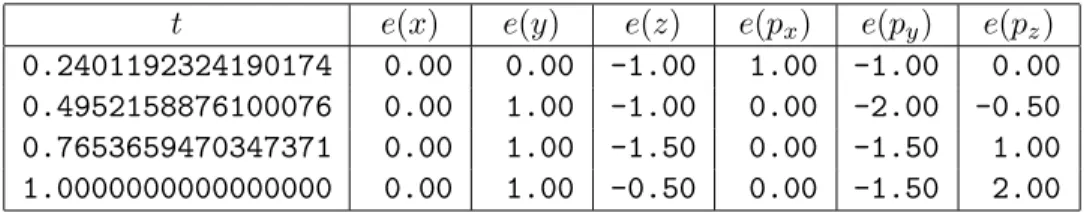
t e(x) e(y) e(z) e(px) e(py) e(pz)
0.2401192324190174 0.00 0.00 -1.00 1.00 -1.00 0.00
0.4952158876100076 0.00 1.00 -1.00 0.00 -2.00 -0.50
0.7653659470347371 0.00 1.00 -1.50 0.00 -1.50 1.00
1.0000000000000000 0.00 1.00 -0.50 0.00 -1.50 2.00
Table 1: Local relative error for an orbit of the RTBP. The first column denotes the time and the remaining ones the relative error for each coordinate, in multiples of the machine precision. See the text for more details.
5.1.1 Local error
We will perform first a numerical integration with the standard double precision of the computer, for 1 unit of time, using a threshold for the error of 10−16, with the step size
algorithm explained in Section 4.3.2 (in this case, the order of the Taylor expansion is 20). To check the accuracy, we have performed the same integration with extended arithmetic (GMP), using the same time step but with a higher order Taylor series (typically, two times the degree used in the double precision integration). To measure the error, we have computed the relative difference between these two approximations. For instance, for the
x coordinate, the exact operations we have implemented are,
e(x) = 1− x˜
x, (14)
wherexis the extended precision approximation and ˜xis the double precision result. All the computations in (14) have been done in double precision. Due to the high level of accuracy, and that we are computing the relative error (in double precision), we have written the result as multiples of the machine precision eps. In our case (an Intel-based computer), eps = 2−52 ≈ 2.22×10⁻¹⁶. Moreover, to evaluate (14) (and only for this
case) we have forced the compiler to produce code such that the result of each arithmetic operation is stored in memory, to avoid using the extra precision available in the registers of the processor.
The results are shown in Table 1: the first column is the time and the remaining columns are the relative error, in multiples of eps, for each coordinate. The “halved” factors (0.50, 1.50, etc) are due to the fact that, due to the roundoff, the smallest (non-zero) number we can obtain from the substraction in (14) is 1
2eps. The reasons for this
extremely small error have been discussed in Section 3.1.
5.1.2 Global error
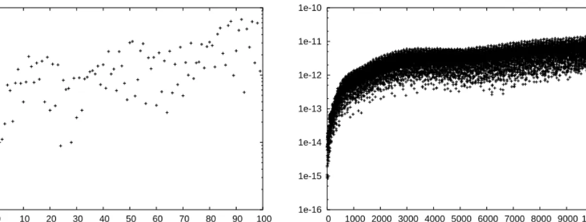
An interesting point is the behaviour of the error for longer integrations. To this end, we will perform two test.
The first test is based on a computation of the local error for a very long time span. We note that, in such a test, there is an extra source of error in the time parametrization of the orbit: even if we force the same time step in both integrations, the different precision
1e-16 1e-15 1e-14 1e-13 0 10 20 30 40 50 60 70 80 90 100 1e-16 1e-15 1e-14 1e-13 1e-12 1e-11 1e-10 0 1000 2000 3000 4000 5000 6000 7000 8000 9000 10000
Figure 2: Error of a numerical integration of the RTBP. The horizontal axis denotes the number of intersections with the Poincar´e section z = 0. Left: the first 100 intersections. Right: 10000 intersections, that correspond to a total integration time of 62837.969279 units. See the text for more details.
introduces an extra time-shift that adds a small error to the comparison. For this reason, during the integration, we have computed the sequence of intersections of the orbit with
z = 0 (the initial condition is already given in this section). Then, for each intersection, we compute the sup norm of the difference between the double and extended arithmetic results to obtain the graphic shown in Figure 2. Looking at these plots, there is a clear propagation of error in the trajectory. We want to note that we are following a quasi-periodic orbit in a region that is almost completely filled by quasiquasi-periodic orbits, each with their own frequencies. This implies that two neighbouring orbits should separate at linear speed. As we are using a log scale in the vertical axis of Figure 2, this drift must have the shape of a log curve which, roughly speaking, coincides with these plots.
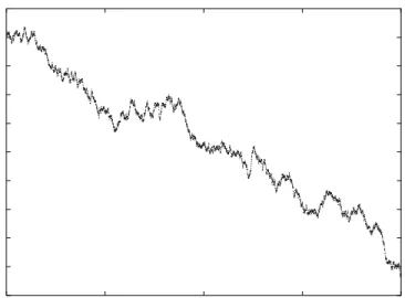
As the Hamiltonian function H is constant on each orbit, a second test is simply to check for its preservation. Although the level of preservation of H does not need to be equal to the error of the integration, checking its preservation is a common test for a numerical integrator. Now we have selected εa=εr = 10−16, with an integration time of
106 units. A first version of the results is shown in Figure 3, where the horizontal axis
denotes the time and the vertical axis is the difference between the actual and the initial value of H, in multiples of eps≈ 2.22×10⁻¹⁶. Although this plot seems to indicate the
presence of a bias in the values of H, we want to point out that the smallness of the drift in H compared to the length of the integration time do not allow to consider this bias meaningful from a statistical point of view. Let us discuss this point in detail. Let
Hj be the value of H at the step number j of the numerical integration and, instead of
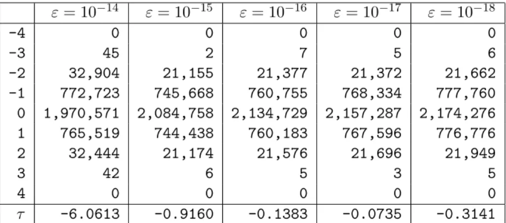
consider Hj −H0, let us focus on the local variation Hj −Hj−1. In Table 2 we show a
summary of the results for the same trajectory as before, but for several local thresholds for the error. To do an standard statistical analysis, let us assume that the sequence of errors Hj −Hj−1 is given by a sequence of independent, identically distributed random
variables, and we are interested in knowing if its mean value is zero or not. Therefore, we will apply the following test of significance of the mean. The null hypothesis assumes
-450 -400 -350 -300 -250 -200 -150 -100 -50 0 50 0 250000 500000 750000 1e+06
Figure 3: Long term behaviour of the energy for local thresholds εr = εa = 10−16.
Horizontal axis: time. Vertical axis: relative variation of the value of the Hamiltonian, in multiples of the machine precision.
that the true mean is equal to zero. If we define
n= X
|k|≤4
νk,
where k denotes a multiple of eps and νk the number of times that this deviation has
occurred, then the sample mean is
m= 1
n
X
|k|≤4
kνk.
and the standard error of the sample mean is
s = s 1 n2 X |k|≤4 (k−m)2ν k.
Under the previous assumptions (independence and equidistribution of the observations), the value
τ = m
s ,
must behave as a N(0,1) standard normal distribution. To test the null hypothesis (i.e., zero mean) with a confidence level of 95%, we have to check for the condition |τ| ≤1.96. The last row of Table 2 shows the value ofτ for the different integrations. It is clear that for ε = 10−14 we must reject that the drift has zero mean, and it is also clear that this
hypothesis cannot be rejected in the other cases.
For the case ε= 10−14 the main source of error is truncation that, from an statistical
ε= 10−14 ε= 10−15 ε= 10−16 ε= 10−17 ε= 10−18 -4 0 0 0 0 0 -3 45 2 7 5 6 -2 32,904 21,155 21,377 21,372 21,662 -1 772,723 745,668 760,755 768,334 777,760 0 1,970,571 2,084,758 2,134,729 2,157,287 2,174,276 1 765,519 744,438 760,183 767,596 776,776 2 32,444 21,174 21,576 21,696 21,949 3 42 6 5 3 5 4 0 0 0 0 0 τ -6.0613 -0.9160 -0.1383 -0.0735 -0.3141
Table 2: Local variation of the energy for several error thresholdsεa=εr ≡ε, during 106
units of time. The first column denotes multiples of the machine precision eps and the remaining columns contain the number of integration steps for which the local variation of energy is equal to the multiple of eps in the first column. The last row is an statistical index to test for zero mean, see the text for details.
then the main source of error turns out to be the roundoff of the underlying arithmetic (see Section 3.1), which looks like a zero mean random process, at least under the standard statistical tests.
A natural question is whether the Taylor method, with a sufficiently small local thresh-old (like 10−16 in the previous example), can compete with a symplectic integrator in the
preservation of the geometrical structure of the phase space of a Hamiltonian system. From a local point of view, we want to note that the Taylor method can deliver machine precision so it is not possible to be “more symplectic”. However, one has to be more careful when extending this reasoning to long term integrations since it is possible that there exist little biases that are only visible in very long integrations. A deeper study is actually in progress.
5.1.3 On the influence of the underlying arithmetic
As an example of the effect of the arithmetic, we will show the different behaviour of the energy. We will use the same trajectory of the RTBP as before, and we will compute the relative variation of the energy. The results for εr = εa = 10−16 using the standard
double precision arithmetic on different hardware are shown in Figure 4. Both graphics show that the error behaviour seem to be dominated by the “noise” of the floating point arithmetic.
5.1.4 Extended precision calculations
We will use the same example as in the previous section. The main difference when generating the code for the Taylor integrator with extended precision is that we have to tell the translator to use extended arithmetic. For instance, to generate code using gmp,
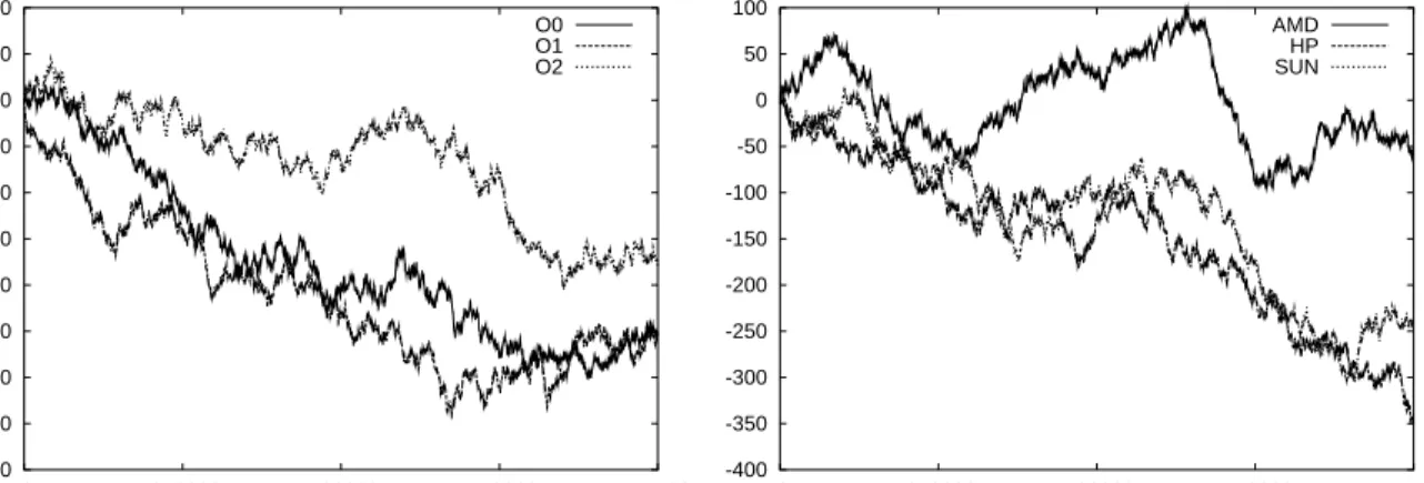
-400 -350 -300 -250 -200 -150 -100 -50 0 50 100 0 250000 500000 750000 1e+06 O0 O1 O2 -400 -350 -300 -250 -200 -150 -100 -50 0 50 100 0 250000 500000 750000 1e+06 AMD HP SUN
Figure 4: Long term behaviour of the energy for local thresholds εr = εa = 10−16. Left
plot: different optimization levels in an Intel processor (the upper curve corresponds to the -O2 option). Right plot: different processors (the upper curve is for the AMD processor). See the text for more details.
t e(x) e(y) e(z) e(px) e(py) e(pz)
1.0000000000000000 0.50 -2.50 -1.00 -0.50 6.50 -5.50
Table 3: Local relative error (in multiples of the machine precision) for an orbit of the RTBP, after a unit of time, using gmp with 256 bits of mantissa. The meaning of the columns is the same as in Table 1. See the text for more comments.
we can do
taylor -name rtbp -o taylor_rtbp.c -step -jet -sqrt rtbp.in taylor -name rtbp -o taylor.h -gmp -header
Note that the first line is exactly the same as for the double precision case, while the arithmetic is only specified in the generation of the header file. The calling routine must take care of setting the desired level of accuracy when initializing the gmp package.
As a first test, we can compute the local error of a numerical integration of the RTBP, as it has been done in Section 5.1.1. We have selected a 256 bits mantissa (this means that the machine precision is eps = 2−256 ≈ 8.636168×10−78), and the value 10−80 for
both the relative and absolute error thresholds. The method has selected a step size near 0.2 and order 94. To obtain the exact solution, we have used a mantissa of 512 bits and an error threshold of 10−155. The local error of the solution after one unit of time (this has
required 4 calls to the Taylor integrator) is shown in Table 3. Comparing with Table 1, we see that the relative error here is a little bit larger. We should note that the double precision arithmetic of the Pentium processor is carried out inside registers having extra accuracy, so it is natural to expect a slightly better behaviour for the roundoff errors.
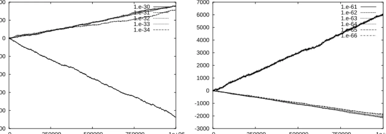
We have also tested the variation of the value of the Hamiltonian for a long-time integration, for different local thresholds. Figure 5 shows the difference between the initial value of the Hamiltonian and its value at each step of integration, for mantissas
-1000 0 1000 2000 3000 4000 5000 6000 7000 8000 9000 0 250000 500000 750000 1e+06 1.e-36 1.e-37 1.e-38 1.e-39 1.e-40 1.e-41 -2000 0 2000 4000 6000 8000 10000 12000 0 250000 500000 750000 1e+06 1.e-75 1.e-76 1.e-77 1.e-78 1.e-79 1.e-80
Figure 5: Long term behaviour of the Hamiltonian for several integrations with gmp arithmetic. The horizontal axis displays the time and the vertical axis shows the variation of the Hamitonian with respect to its initial value. Left plot: results for gmp arithmetic with a 128 bits mantissa, and several local thresholdsεa=εr =εas shown in the graphic.
Right plot: results for gmp arithmetic with a 256 bits mantissa. See the text for more details.
of 128 (left) and 256 (right) bits. The differences are shown in multiples of the machine precision of each arithmetic. The lower curve on these plots corresponds to the largest threshold (εa =εr = 10−36 and εa =εr = 10−75 for the left and right plot, respectively)
where the main source of error is the truncation of the Taylor series. The remaining curves correspond to smaller thresholds for which the error mainly comes from the roundoff of the gmp arithmetic. We clearly see the different behaviour of these two sources of error, as well as the drift introduced by the roundoff of the artihmetic.
We have also tested the preservation of the Hamiltonian for a different extended arith-metic, the qd library. The results are shown in Figure 6. Again, we have used the dd realtype (two doubles) for the left plot andqd realtype (four doubles) for the right one. For this arithmetic, it does not make sense to use the machine precision as a unit for the error.1. Hence, we have simply multiplied the differences in the Hamiltonian by
1032 (dd real) and 1064 (qd real). In the left plot, the bottom curve corresponds to
εa=εr = 10−30 to the largest error threshold while the effect of the truncation dominates
the error. The remaining curves show the behaviour of the roundoff error of the arith-metic. In the right plot, is the upper curve that corresponds to the largest error threshold (in this case, εa =εr = 10−61) showing the effect of the truncation error. The remaining
curves show the drift due to the roundoff of the arithmetic.
5.2
Speed
There is plenty of numerical methods in the literature, and we do not plan to survey all of them but simply to compare our implementation of Taylor method against a few well 1Add realnumber is defined as the sum of two doubles. Therefore, the sum 1 +εis always different from 1 as long asεcan be represented in a double.
-10000 -8000 -6000 -4000 -2000 0 2000 4000 0 250000 500000 750000 1e+06 1.e-30 1.e-31 1.e-32 1.e-33 1.e-34 -3000 -2000 -1000 0 1000 2000 3000 4000 5000 6000 7000 0 250000 500000 750000 1e+06 1.e-61 1.e-62 1.e-63 1.e-64 1.e-65 1.e-66
Figure 6: Long term behaviour of the Hamiltonian for several integrations with qd arith-metic. The horizontal axis displays the time and the vertical axis shows the variation of the Hamitonian with respect to its initial value. Left plot: results for dd real arith-metic (nearly 32 decimal digits), and several local thresholds εa=εr =εas shown in the
graphic. Right plot: results for the qd real arithmetic (nearly 64 decimal digits). See the text for more details.
known methods. A characteristic of these methods is that they have a freely available implementation, which is the one we have used. These implementations are coded in FORTRAN77, which adds an extra difficulty on the comparisons, since the observed differences may come from the different compilers. Therefore, to help the readers with these comparisons, the package includes the code for all the examples, so that they can be run on any combination of compiler/computer for comparisons.
Our tests have been done in a GNU/Linux workstation, with an Intel Pentium III processor running at 500 MHz. We have used the following GNU compilers:
$ gcc -v
gcc version 2.95.4 20011002 (Debian prerelease) $ g77 -v
g77 version 2.95.4 20011002 (from FSF-g77 version 0.5.25 20010319) The methods considered are dop853, an explicit Runge-Kutta code of order 8, and odex, an extrapolation method of varying order based on the Gragg-Bulirsh-Stoer al-gorithm. Both methods are documented in [HNW00] and the code we have used is the one contained in this book, that can be downloaded from E. Hairer’s web page, http://www.unige.ch/math/folks/hairer/software.html. We note that extrapola-tion methods are similar to Taylor in the sense that they can use arbitrarily high orders, so they are the natural methods to compare with.
For the tests, we have used three vector fields: the RTBP, the Lorenz system, a periodically forced pendulum, and the RTBP. The equations for the Lorenz system are
˙
x = 10(y−x),
˙
˙
z = xy− 8
3z, and the equations for the forced pendulum are
˙
x = y,
˙
y = −sin(x)−0.1y+ 0.1 sin(t)
The RTBP (see equations (13)) has been coded as in Figure 1 so that, in all the cases, the vector field has the same number of operations.
As before, we have used the same formulas to code the vector fields for dop853, odex and taylor.
A first possibility to make the comparisons is to set the same threshold for all the methods and then compare the speeds. Note that, as the algorithms for the step size selection are completely different, one of them could be more “conservative” than the others and predict (unnecessarily) smaller step sizes so that the comparisons would be meaningless. For this reason we have proceeded in the following way: given an initial condition, we can compute the corresponding orbit during, say, 16 units of time and to compare the final point with the true value to obtain the real absolute error.2 In Table 4
we show the computer time and final error for the three methods, using different thresholds for the step size control. To have a measurable running time, the program repeats the same calculation 1000 times.
Therefore, we ignore the column labelled ε (the error threshold used for the step size control), and we only compare the computing time to achieve a prescribed accuracy (this is equivalent to compare the accuracy obtained for a fixed computing time). The results clearly show the effectiveness of the Taylor method for these examples.
5.2.1 A simple comparison with ADOL-C
ADOL-C is a public domain package for automatic differentiation. The main differences between the automatic differentiation of our package and ADOL-C are:
a) ADOL-C is a general purpose package, while taylor is specifically designed for the numerical integration of ODEs.
b) The input of ADOL-C is a C/C++ function (with some restrictions in the grammar used), whiletaylorhas its own input grammar, which is a little bit more restrictive. c) ADOL-C does not include code for the step size control. This means that ADOL-C can only be used to generate the Taylor coefficients and the user must supply code for the order and step size control.
For this reason, we will only test the speed of the generation of the Taylor coefficients. As before, the tests have been done on an Intel Pentium III running at 500 MHz, using ADOL-C version 1.8.7. The examples considered are the Lorenz system, RTBP, 2The true value has been obtained from an integration with the Taylor method using thegmparithmetic with mantissas of 128 and 256 bits.
Lorenz
dop583 odex taylor
ε time error ε time error ε time error
1.e-10 7.01 5.9e-03 1.e-10 8.73 6.2e-02 1.e-10 7.61 3.1e-06 1.e-11 8.91 5.0e-04 1.e-11 10.11 3.3e-03 1.e-11 7.99 4.4e-07 1.e-12 11.65 4.3e-05 1.e-12 11.54 2.0e-04 1.e-12 8.40 4.8e-08 1.e-13 15.31 3.7e-06 1.e-13 12.74 5.8e-06 1.e-13 8.80 3.3e-08 1.e-14 20.19 1.2e-06 1.e-14 15.04 6.4e-06 1.e-14 9.22 3.4e-08 1.e-15 26.76 8.9e-07 1.e-15 17.81 3.7e-06 1.e-15 9.75 9.2e-09 1.e-16 35.51 9.5e-07 1.e-16 50.47 1.9e-06 1.e-16 10.75 7.5e-09
Perturbed pendulum
dop583 odex taylor
ε time error ε time error ε time error
1.e-10 0.62 3.4e-11 1.e-10 1.49 6.9e-10 1.e-10 0.38 2.8e-13 1.e-11 0.78 3.6e-12 1.e-11 1.70 4.9e-11 1.e-11 0.42 2.1e-14 1.e-12 1.03 3.1e-13 1.e-12 1.93 1.7e-12 1.e-12 0.44 7.6e-15 1.e-13 1.38 2.7e-14 1.e-13 2.17 9.1e-14 1.e-13 0.47 1.2e-15 1.e-14 1.83 2.3e-15 1.e-14 2.36 4.4e-15 1.e-14 0.48 8.7e-16 1.e-15 2.45 2.1e-15 1.e-15 2.68 3.1e-15 1.e-15 0.52 5.8e-16 1.e-16 3.24 3.2e-15 1.e-16 3.09 1.1e-14 1.e-16 0.59 3.8e-16
RTBP
dop583 odex taylor
ε time error ε time error ε time error
1.e-10 1.43 1.1e-09 1.e-10 1.74 1.8e-09 1.e-10 1.68 6.2e-12 1.e-11 1.84 9.4e-11 1.e-11 2.02 9.2e-11 1.e-11 1.86 4.6e-13 1.e-12 2.44 8.6e-12 1.e-12 2.43 2.4e-11 1.e-12 2.08 4.4e-14 1.e-13 3.24 8.0e-13 1.e-13 2.74 3.7e-13 1.e-13 2.27 7.2e-15 1.e-14 4.32 7.5e-14 1.e-14 3.14 1.5e-13 1.e-14 2.50 4.2e-15 1.e-15 5.73 9.9e-15 1.e-15 3.71 2.4e-13 1.e-15 2.82 1.7e-15 1.e-16 7.63 2.0e-15 1.e-16 4.85 1.3e-13 1.e-16 3.26 5.8e-15 Table 4: Speed comparison betweendopri853,odexandtaylor. εis the selected thresh-old for the error (both relative and absolute threshthresh-olds have been set to the same value), computer time is given in seconds, and the error is the absolute error at the end point of the integration. To have a measurable computer time, we have repeated the same integration 1000 times. See the text for more details.
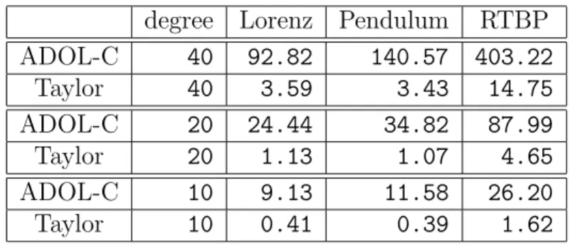
degree Lorenz Pendulum RTBP ADOL-C 40 92.82 140.57 403.22 Taylor 40 3.59 3.43 14.75 ADOL-C 20 24.44 34.82 87.99 Taylor 20 1.13 1.07 4.65 ADOL-C 10 9.13 11.58 26.20 Taylor 10 0.41 0.39 1.62
Table 5: Time (in seconds) to compute 100,000 times the jet of derivatives for the Lorenz system, a periodically forced pendulum and the RTBP.
the Lorenz system and a periodically forced pendulum. To measure the time, we have computed the jet of derivatives 100,000 times. The results are contained in Table 5, and clearly show the efficiency of taylor.
6
Conclusions
In this paper we have discussed a new publicly available implementation of the classical Taylor method for the numerical solution of ODEs. This program reads the differen-tial equations from a file and outputs a complete Taylor integrator (including adaptive selection of degree and step size) for the given system.
The package has been tested against freely available implementations of two well-known numerical integrators. We do not claim that the results from these tests can be extrapolated to any example, but simply that taylor can be very competitive in many situations. We believe that the fact that the the methods used for the comparisons are coded in FORTRAN 77 while the output of taylor is ANSI C has a small impact in the results. However, the package includes the source code used for tests, so that the user can try them with different compilers/computers. In fact, the best way to know whether taylor is suitable for a concrete application, with a given compiler and computer, is simply to try it.
Finally, let us remark that one of the strong points of the package is the support for extended precision arithmetic.
Acknowledgements
The authors want to thank R. Broucke, R. de la Llave and C. Sim´o for their comments. This work has been supported by the Comisi´on Conjunta Hispano Norteamericana de Co-operaci´on Cient´ıfica y Tecnol´ogica. A.J. has also been supported by the MCyT/FEDER grant BFM2003-07521-C02-01, the Catalan CIRIT grant 2001SGR–70 and DURSI.
References
[Bar80] D. Barton. On Taylor series and stiff equations. ACM Trans. Math. Software, 6(3):280–294, 1980.
[BBCG96] M. Berz, C. Bischof, G.F. Corliss, and A. Griewank, editors. Computational Differentiation: Techniques, Applications, and Tools. SIAM, Philadelphia, Penn., 1996.
[BCCG92] C.H. Bischof, A. Carle, G.F. Corliss, and A. Griewank. ADIFOR: Automatic differentiation in a source translation environment. In Paul S. Wang, editor, Proceedings of the International Symposium on Symbolic and Algebraic Com-putation, pages 294–302, New York, 1992. ACM Press.
[BKSF59] L.M. Beda, L.N. Korolev, N.V. Sukkikh, and T.S. Frolova. Programs for automatic differentiation for the machine BESM. Technical Report, Insti-tute for Precise Mechanics and Computation Techniques, Academy of Science, Moscow, USSR, 1959. (In Russian).
[Bro71] R. Broucke. Solution of the N-Body Problem with recurrent power series. Celestial Mech., 4(1):110–115, 1971.
[BWZ70] D. Barton, I.M. Willers, and R.V.M. Zahar. The automatic solution of or-dinary differential equations by the method of Taylor series. Computer J., 14(3):243–248, 1970.
[CC82] G.F. Corliss and Y.F. Chang. Solving ordinary differential equations using Taylor series. ACM Trans. Math. Software, 8(2):114–144, 1982.
[CC94] Y.F. Chang and G.F. Corliss. ATOMFT: Solving ODEs and DAEs using Taylor series. Computers and Mathematics with Applications, 28:209–233, 1994.
[CGH+97] G.F. Corliss, A. Griewank, P. Henneberger, G. Kirlinger, F.A. Potra, and H.J.
Stetter. High-order stiff ODE solvers via automatic differentiation and rational prediction. In Numerical analysis and its applications (Rousse, 1996), pages 114–125. Springer, Berlin, 1997.
[Cor95] G.F. Corliss. Guaranteed error bounds for ordinary differential equations. In M. Ainsworth, J. Levesley, W. A. Light, and M. Marletta, editors, Theory of Numerics in Ordinary and Partial Differential Equations, pages 1–75. Oxford University Press, Oxford, 1995. Lecture notes for a sequence of five lectures at the VI-th SERC Numerical Analysis Summer School, Leicester University, 25 - 29 July, 1994.
[GC91] A. Griewank and G.F. Corliss, editors. Automatic Differentiation of Algo-rithms: Theory, Implementation, and Application. SIAM, Philadelphia, Penn., 1991.
[Gib60] A. Gibbons. A program for the automatic integration of differential equations using the method of Taylor series. Comp. J., 3:108–111, 1960.
[Gri00] A. Griewank. Evaluating Derivatives. SIAM, Philadelphia, Penn., 2000. [HNW00] E. Hairer, S. P. Nørsett, and G. Wanner. Solving ordinary differential
equa-tions I. Nonstiff problems, volume 8 ofSpringer Series in Computational Math-ematics. Springer-Verlag, Berlin, second revised edition, 2000.
[Hoe01] J. Hoefkens.Rigorous numerical analysis with high order Taylor methods. PhD thesis, Michigan State University, 2001.
[IS90] D.H. Irvine and M.A. Savageau. Efficient solution of nonlinear ordinary dif-ferential equations expressed in S-system canonical form. SIAM J. Numer. Anal., 27(3):704–735, 1990.
[JZ85] F. Jalbert and R.V.M. Zahar. A highly precise Taylor series method for stiff ODEs. In Proceedings of the fourteenth Manitoba conference on numerical mathematics and computing (Winnipeg, Man., 1984), volume 46, pages 347– 358, 1985.
[KC92] G. Kirlinger and G.F. Corliss. On implicit Taylor series methods for stiff ODEs. In Computer arithmetic and enclosure methods (Oldenburg, 1991), pages 371–379. North-Holland, Amsterdam, 1992.
[MH92] K.R. Meyer and G.R. Hall. Introduction to Hamiltonian Dynamical Systems and the N-Body Problem. Springer, New York, 1992.
[Moo66] R.E. Moore. Interval Analysis. Prentice-Hall, Englewood Cliffs, N.J., 1966. [MS99] R. Mart´ınez and C. Sim´o. Simultaneous binary collisions in the planar
four-body problem. Nonlinearity, 12(4):903–930, 1999.
[NJC99] N.S. Nedialkov, K.R. Jackson, and G.F. Corliss. Validated solutions of ini-tial value problems for ordinary differenini-tial equations. Appl. Math. Comput., 105(1):21–68, 1999.
[Ral81] L.B. Rall. Automatic Differentiation: Techniques and Applications, volume 120 of Lecture Notes in Computer Science. Springer Verlag, Berlin, 1981. [Sim] C. Sim´o. Dynamical properties of the figure eight solution of the three–body
problem. To appear in A. Chenciner, R. Cushman, C. Robinson and Z. Xia, editors, Proceedings of the Chicago Conference dedicated to Don Saari. [Sim01] C. Sim´o. Global dynamics and fast indicators. In H.W. Broer, B. Krauskopf,
and G. Vegter, editors, Global analysis of dynamical systems, pages 373–389, Bristol, 2001. IOP Publishing.
[Ste56] J.F. Steffensen. On the restricted problem of three bodies. Danske Vid. Selsk. Mat.-Fys. Medd., 30(18):17, 1956.
[Ste57] J.F. Steffensen. On the problem of three bodies in the plane. Mat.-Fys. Medd. Danske Vid. Selsk., 31(3):18, 1957.
[SV87] M.A. Savageau and E.O. Voit. Recasting nonlinear differential equations as
S-systems: a canonical nonlinear form. Math. Biosci., 87(1):83–115, 1987. [SV01] C. Sim´o and C. Valls. A formal approximation of the splitting of
separatri-ces in the classical Arnold’s example of diffusion with two equal parameters. Nonlinearity, 14(4):1707–1760, 2001.
[Sze67] V. Szebehely. Theory of Orbits. Academic Press, 1967.
[Wen64] R. E. Wengert. A simple automatic derivative evaluation program. Comm. ACM, 7(8):463–464, 1964.