May 2011, Volume 41, Issue 2. http://www.jstatsoft.org/
The
STAMP
Software for State Space Models
Roy Mendelssohn NOAA/NMFS/SWFSC/PFEL
Abstract
This paper reviews the use of STAMP (Structural Time Series Analyser, Modeler and Predictor) for modeling time series data using state-space methods with unobserved components. STAMPis a commercial, GUI-based program that runs on Windows, Linux and Macintosh computers as part of the largerOxMetricsSystem. STAMPcan estimate a wide-variety of both univariate and multivariate state-space models, provides a wide array of diagnostics, and has a batch mode capability. The use of STAMPis illustrated for the Nile river data which is analyzed throughout this issue, as well as by modeling a variety of oceanographic and climate related data sets. The analyses of the oceanographic and climate data illustrate the breadth of models available in STAMP, and that state-space methods produce results that provide new insights into important scientific problems.
Keywords:STAMP, state space methods, unobserved components, Nile river, Pacific decadal oscillation, north Pacific high, El Ni˜no.
1.
STAMP
STAMP (Structural Time Series Analyser, Modeler and Predictor) is a commercial, graph-ical user interface (GUI)-based package for the analysis of both univariate and multivariate state-space models written byKoopman, Harvey, Doornik, and Shephard(2009). It runs on Windows, Macintosh and Linux operating systems as part of the largerOxMetrics System, a software system for (econometric) data analysis and forecasting (Doornik 2009). The au-thors are some of the leading researchers in the field of state-space modeling, and as such the algorithms used inSTAMP, as well as the features available for analysis of model fit, tend to stay current with the state of the art in the literature.
A strength ofSTAMPis the large variety of models that can be analyzed, both univariate and multivariate. The univariate models include structural component models as well as time-varying regressions, and the multivariate models include “common trends”, “common cycles”, “common seasons” and “seemingly unrelated time series equations” (SUTSE), with
exoge-and interventions by equation, to define separate dependence structures for each component, provides for a wide choice of variance matrices, and permits higher order multivariate com-ponents. Only some of these features are illustrated in this article, but STAMP provides a complete package for linear, Gaussian state-space model estimation.
OxMetrics integrates STAMP into a larger class of related models, and provides a broad suite of graphics, data transformation options, and data arithmetic options. And although STAMP is primarily GUI-based,OxMetrics provides a language for batch processing. Even more so, as shown below, as a model is created in the GUI,STAMPgenerates the code that will produce the same model in batch mode.
In Section 2 the Nile river data, that are analyzed in all the articles in this special issue, are modeled usingSTAMP. For purposes of “full disclosure” the Nile river data are analyzed extensively in the manual that comes withSTAMP8.2, and the analysis in Section 2 follows the analysis therein. Even so, all the steps in the analysis are straightforward given the tools provided by STAMP and the end result would be the same with or without the analysis in the manual. All the analyses in Section 2 were done using STAMP 8.2 on a 2.2 GHz Intel Core 2 Duo Macbook Pro, and all graphics in that section are either unretouched from what is produced inSTAMP8.2 or use features for editing the graphics that are supplied by OxMetrics. In Section 3 oceanographic and climate indices are analyzed using state-space models in an area where the uses of these methods are just beginning to come to fore. In Section4state-space models are combined with subspace identification techniques to analyze a large-scale space-time dataset.
2. Nile river
OxMetrics can import a variety of formats including Excel and Lotus spreadsheets, comma separated (.csv) files, Gauss and Stata files, a variety of text formats as well as its own native format. The Nile river volume data were provided in one of the text file formats that OxMetricssupports, making import of the data easy. As part of the data import, the time and time interval of the data are defined, and that information is carried along in the rest of the analyses and graphics. STAMPis started within OxMetrics.
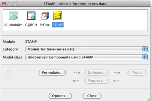
The initial STAMP dialog (Figure 1) allows the user to select other dialogs that change options or settings for the various stages of data modeling. Selecting “Formulate” to define the initial model, a screen comes up allowing the user to choose which variables to include in the model, and what role they will play (“X” or “Y”), the latter being necessary for certain classes of models, such as a state-space model with a fixed effect or a time-dependent regression (Figure2).
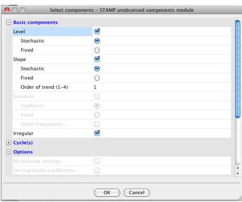
Having chosen which variables to use in the model, a dialog comes up with options for what components to include in the model (Figure3).
A nice feature of STAMP is the wide range of models that can be estimated, and the fact that it is kept up-to-date with new research, such as allowing higher “orders” in both the level and the cycle (seeHarvey and Trimbur 2003). Kitagawa and Gersch(1996, for example) have long advocated that many series are better fit with a higher order of differencing in the level
Figure 1: Initial window when startingSTAMP from withinOxMetrics.
Figure 2: Window in STAMP for choosing the variables to be included in the analysis and the role the variables will play in the analysis.
Figure 3: Window inSTAMP for selecting model components. Value q ratio
Level 1469.18 0.09731 Irregular 15098.5 1.000
Table 1: Maximum likelihood estimates of the variances in the local level model for the Nile river data. The q ratio is the relative variance of the level and irregular, that is, the signal-to-noise ratio.
term. The default model is the “basic structural model” (BSM), a model which includes a stochastic level and slope as well as a stochastic seasonal component, and a BSM without the seasonal component was used as the initial model to estimate the Nile river data. In the notation of equation (4) in Commandeur, Koopman, and Ooms(2011) the initial model is:
yt = µt+t (1)
µt+1 = µt+νt+ξt (2)
νt+1 = νt+ζt. (3)
For this model the maximum likelihood estimate of the slope was zero (with no variance), so the model was re-estimated with just a stochastic local level (Table1).
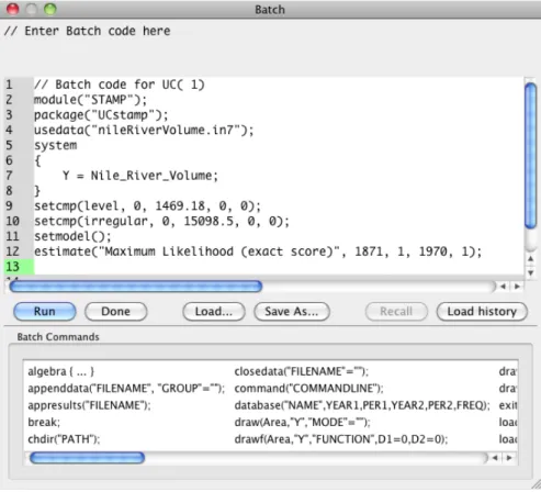
An important feature ofSTAMPis that although it is GUI based, it also can be run in batch mode using a scripting language that is part of OxMetrics. Even more so, as you select a model in the GUI, STAMP automatically generates the code needed to run that model in
Figure 4: Window showing the generated code for batch processing of the local level model withinSTAMP.
batch mode (Figure4). This is a feature used in Section4.
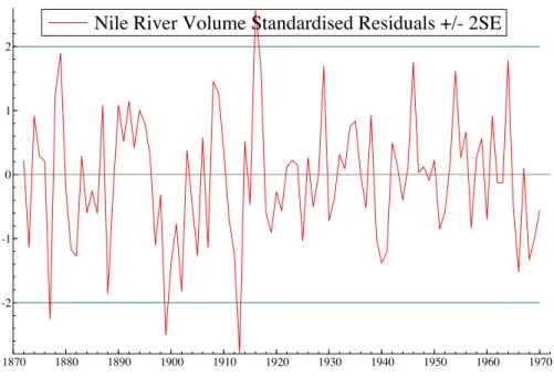
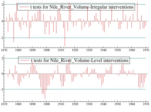
The estimated local level model (Figure 5) suggests a mean level that is relatively constant over long periods with several possible shifts, and this impression is reinforced in the plots of the standardized residuals (Figure6) and even more so in the auxiliary residuals (Figure 7). STAMPhas a feature to automatically detect possible points of intervention in a series, and the local level model was re-estimated with this feature. A level break in 1899 and an outlier break in 1913 are identified by this automatic feature, the former corresponding to the building of the Aswan dam, and the latter to a year of extremely low flow in several African rivers following the high-latitude Katmai eruption.
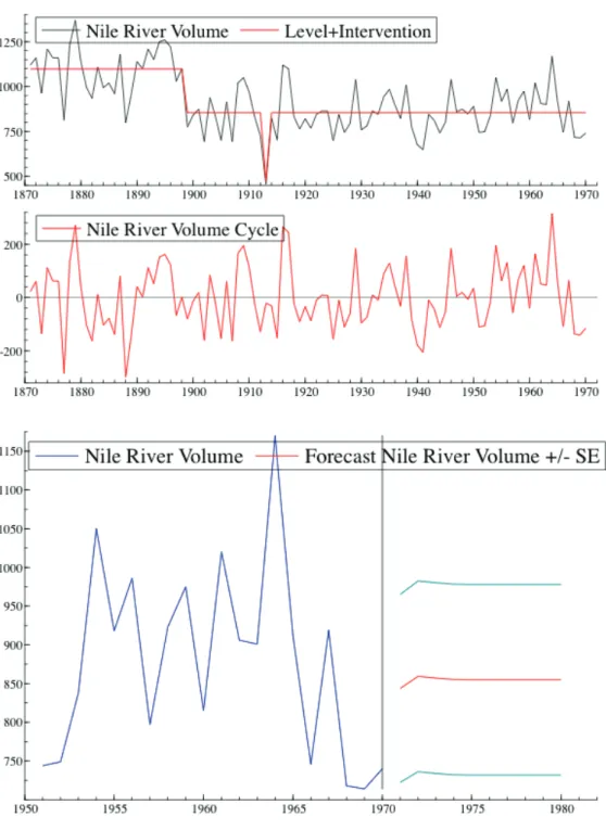
Re-estimating the local level model to include the interventions produces a model where the level changes only due to the interventions (Table2) but the residual graphs show significant autocorrelations and other signs of periodicity in the residuals. Based on this, a final model was fit with a fixed level, a stochastic cycle, and the two interventions (Table3). A stochastic cycle, in the notation of equation (6) inCommandeur et al.(2011) is defined as:
ψt ψt∗ =ρ cosλc sinλc −sinλc cosλc ψt−1 ψt∗−1 + κt κ∗t , t= 1, . . . , T, (4)
whereψt and ψt∗ are the states, λc is the frequency, in radians, in the range 0< λc ≤π,κt andκ∗t are two mutually uncorrelated white noise disturbances with zero means and common varianceσ2κ, andρis a damping factor. The damping factorρin (1) accounts for the time over
Nile River Volume Level +/- 2SE
1870 1880 1890 1900 1910 1920 1930 1940 1950 1960 1970 500
750 1000
1250 Nile River Volume Level +/- 2SE
Nile River Volume Level +/- 2SE
1870 1880 1890 1900 1910 1920 1930 1940 1950 1960 1970 800
1000
1200 Nile River Volume Level +/- 2SE
Figure 5: Nile local level model components with confidence intervals.
Nile River Volume Standardised Residuals +/- 2SE
1870 1880 1890 1900 1910 1920 1930 1940 1950 1960 1970 -2
-1 0 1
2 Nile River Volume Standardised Residuals +/- 2SE
Value q ratio Level 0.00000 0.00000 Irregular 14124.7 1.000
Coefficient RMSE tvalue Prob Outlier 1913(1) −399.52109 119.68141 −3.33821 [0.00120] Level break 1899(1) −242.22887 26.52156 −9.13328 [0.00000]
Table 2: Maximum likelihood estimates of the variance and regression terms in the local level model with interventions for the Nile river data. RMSE is the residual mean square error and theq ratio is the relative variance of the level and irregular, that is, the signal-to-noise ratio.
t tests for Nile_River_Volume-Irregular interventions
1870 1880 1890 1900 1910 1920 1930 1940 1950 1960 1970 -2
0
2 t tests for Nile_River_Volume-Irregular interventions
t tests for Nile_River_Volume-Level interventions
1870 1880 1890 1900 1910 1920 1930 1940 1950 1960 1970 -2
0
2 t tests for Nile_River_Volume-Level interventions
Figure 7: Nile local level model auxiliary residuals.
which a higher amplitude event (consider this to be a “shock” to the series) in the stochastic cycle will contribute to subsequent cycles. A stochastic cycle has changing amplitude and phase, and becomes a first order autoregression if λc is 0 or π. Moreover, it can be shown that as ρ→ 1, then σκ2 →0 and the stochastic cycle reduces to the stationary deterministic cycle:
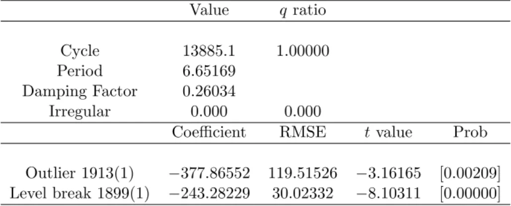
ψt=ψ0cosλct+ψ∗0sinλct, t= 1, . . . , T. (5) The cycle has a period of 6.65 years and a damping factor of 0.26034 (Figure8), and all of the test statistics (Table 4), residual diagnostics (Figures 9), and auxiliary residual diagnostics
Figure 8: Nile cycle model with interventions.
(Figure 10) for this model suggest a good fit both to the data and to the assumptions of the model. The roughly seven year cycle is consistent with a number of processes in the atmo-sphere and ocean, and conditions in the Nile have been correlated with drought conditions in the Southwest United States, for example, based on these teleconnections (Cayan, Dettinger, Diaz, and Graham 1998;Jiang, Mendelssohn, Schwing, and Fraedrich 2002).
Value q ratio Cycle 13885.1 1.00000 Period 6.65169
Damping Factor 0.26034
Irregular 0.000 0.000
Coefficient RMSE tvalue Prob Outlier 1913(1) −377.86552 119.51526 −3.16165 [0.00209] Level break 1899(1) −243.28229 30.02332 −8.10311 [0.00000]
Table 3: Maximum likelihood estimates of the variance and regression terms in the cycle with interventions model for the Nile river data.
Summary statistics Nile river volume
T 100.00 p 4.0000 Std. error 118.68 Normality 0.36671 H(32) 0.80242 DW 1.9483 r(1) 0.011016 q 12.000 r(q) −0.070861 Q(q, q−p) 5.7131 R2 0.51811
Table 4: Test statistics for the cycle with interventions model for the Nile river data. T is the number of time periods, p the number of parameters,std.error is the square root of the prediction error variance,N ormality is the Bowman-Shenton statistic of the third and fourth moments of the residuals,H(32) is a measure of heteroskedasticity,DW is the Durbin-Watson test,r(1) is the estimated residual lag 1 autocorrelation,Q(q, q−p) is the Box-Ljung statistic based on the firstq autocorrelations,r(q) is the lag q autocorrelation, and R2 is a goodness of fit measure.
0 5 10 15 20 -0.5 0.0 0.5 -3 -2 -1 0 1 2 3 0.1 0.2 0.3 0.4 resid × normal -2 -1 0 1 2 -2 -1 0 1 2 3 QQ plot
resid × normal Nile River Volume Cusum Residuals
1880 1900 1920 1940 1960 -10
0
10 Nile River Volume Cusum Residuals
Figure 9: Nile cycle model showing the variety of residual diagnostics available inSTAMP.
t tests Nile River Irregular interventions
1880 1900 1920 1940 1960 -2
0
2 t tests Nile River Irregular interventions t tests Nile River Irregular interventions N(s=0.999)
-3 -2 -1 0 1 2 3
0.2
0.4 Densityt tests Nile River Irregular interventions N(s=0.999)
t tests Nile River Irregular interventions × normal
-2 -1 0 1 2
-2 0 2
QQ plot
t tests Nile River Irregular interventions × normal t tests Nile River Level interventions
1880 1900 1920 1940 1960 0
2 t tests Nile River Level interventions
t tests Nile River Level interventions N(s=0.707)
-2 -1 0 1 2
0.25 0.50
Density
t tests Nile River Level interventions N(s=0.707) t tests Nile River Level interventions × normal
-1.0 -0.5 0.0 0.5 1.0 1.5 2.0 -1
0 1 2 QQ plot
t tests Nile River Level interventions × normal
Figure 10: Auxiliary residual diagnostics for the Nile cycle model showing the variety of diagnostic tools available inSTAMP.
3. Ocean and climate indices
New statistical methods are often demonstrated to produce results that differ from those of previous methods, but it is unclear that these differences are of any importance to the subject matter at hand. In this section, we use state-space methods to examine oceanographic and climate related indices, and show that the use of these models produce significant scientific insight. All of the univariate modeling was done usingSTAMP, while the subspace identifi-cation procedure was performed inMATLABon the output from univariate models estimated by STAMP.
3.1. Pacific decadal oscillation
The Pacific decadal oscillation (PDO) is defined as the first principal component (or as called in the oceanography literature “Empirical orthogonal function” or “EOF”) of monthly 5-degree sea surface temperature (SST) anomalies after removal of the monthly global mean of the anomalies (Mantua, Hare, Zhang, Wallace, and Francis 1997). There has been much discussion as to what the PDO represents, with some authors calling any decadal-scale dynamic in the ocean the PDO, while others say the PDO is simply red noise (autoregressive) and is consistent with an oceanographic model where the atmosphere is white and the ocean is red (see for example Pierce 2001;Rudnick and Davis 2003). If the latter is true, the PDO is stationary and does not represent any shifts in the climate dynamics.
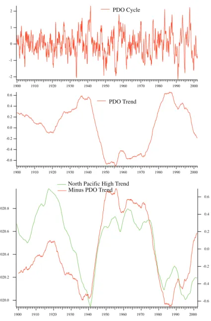
To examine this question, a series of models were estimated for the PDO, including models with a fixed and a stochastic level, models with a fixed and a stochastic seasonal component, and each of those in combination with an AR(1) component and a stochastic cycle. This type of analysis can be readily carried out in STAMP given the large class of models and model statistics it provides and by utilizing the batch language to automate the estimation of the different models. The “best” model, based on AIC and BIC statistics as well as examination of the residuals, was a model with a stochastic level, a stochastic cycle, and a fixed seasonal component (Figure 11). What is clear is that while the largest amount of the variance is contained in the higher frequency stochastic cycle term, there is a significant trend in the series.
The same set of analyses that were carried out for the PDO were also done for an index of the north Pacific high (NPH) pressure center, with the same model (stochastic level, stochastic cycle, and fixed seasonal) being selected as the best model. The estimated levels in the two series (Figure 11) as well as the estimated stochastic cycles (not shown) are almost identical. So while there is a significant trend and cyclic component in the PDO, these components are capturing the dynamics in the region of the north Pacific influenced by the NPH. An interesting question is to what degree the feedback occurs in each direction (the ocean influencing the atmosphere or the atmosphere influencing the ocean).
3.2. El Ni˜no
This section follows Mendelssohn, Bograd, Schwing, and Palacios (2005). There has been recent speculation that El Ni˜no events, at least measured by two indices, the southern os-cillation index (SOI) (see for example Philander 1990) and the NINO3 index (Mann, Gille, Bradley, Hughes, Overpeck, Keimig, and Gross 2000), have been increasing both in frequency and intensity over time (see for example Trenberth and Hoar 1997). The SOI is defined as
1020.8 1020.6 1020.4 1020.2 1020.0 2000 1990 1980 1970 1960 1950 1940 1930 1920 1910 1900 0.6 0.4 0.2 0.0 -0.2 -0.4 -0.6 North Pacific High Trend
Minus PDO Trend 1 0 -1 -2 2000 1990 1980 1970 1960 1950 1940 1930 1920 1910 1900 -0.6 -0.4 -0.2 0.0 0.2 0.4 0.6 2000 1990 1980 1970 1960 1950 1940 1930 1920 1910 1900 PDO Trend
Figure 11: Estimated cycle and level for the Pacific decadal oscillation (PDO) and comparison with the estimated north Pacific high (NPH) level.
the anomalies of the difference in the pressure at Darwin, Australia and Tahiti. The relative change in the pressures is believed to be associated with shifts in the wind fields, and a nega-tive anomaly signifying El Ni˜no periods while a positive anomaly signifying La Ni˜na periods. The NINO3 series is defined as the average sea surface temperature over a large area of the tropical Pacific, viewed as a measure of the overall surface heat in the tropical Pacific waters. It has been suggested that the NINO3 is exhibiting an increased frequency of warm events. To examine these questions, the same estimation process used in Section 3.1 was used to estimate a “best fit” model for the NINO3 series, for the SOI, and for the component series of
c. Cycles Darwin Tahiti Darwin Tahiti 57-58 65-66 72-7376-77 82-83 86-8791-92 97-98
d. Cycles and El Niño
Darwin
SOI Nino3NOI a. Trends
b. Nino3 Trend and Trend + Cycle
°C
°C
Figure 12: a. The estimated trend terms for the negative of the southern oscillation index (SOI) (blue, [−0.58,0.019]), Darwin pressure (red, [97.8,101.25]), yearly NINO3 (green, [−0.104,0.575]), and the negative of the northern oscillation index (NOI)I (black, [−0.53,0.53]). The numbers in brackets give the range of each of the variables on the y-axis. b. The estimated NINO3 trend (black) and trend plus stochastic cycle (red). c. Stochastic cycles for Darwin (red) and Tahiti (blue). d. Stochastic cycles for Darwin and Tahiti, and El Ni˜no events.
the SOI (i.e., the Darwin and Tahiti pressures). Again the local level model with a stochastic cycle term was the best fit to the data, except for the Tahiti pressure series where a fixed level model was preferred over a model with a stochastic level. The trends in the series are very similar (Figure 12a,b), in particular the Darwin pressure trend and the SOI trend, which is not surprising since Tahiti pressure has a constant mean. What is more surprising is that the stochastic cycles are very close (Figure12c), and the El Ni˜no events can be discerned equally as well if not better just from Darwin pressures rather than from the more complicated index (Figure12d). The smoothed residuals for the stochastic cycle suggest that more recent events are in the tails of the distributions, but the overall impression from the residual and auxiliary residual plots is that this model provides a reasonable fit to the data series. Since the stochastic cycle is stationary, this analysis shows no significant increase in the frequency of El Ni˜no events. Rather there has been warming trend in tropical SST, and this has caused SST anomalies to similarly increase.
by defining “common trends” or “common cycles”, parameterized the same way but of lower dimension than the observed data (see for exampleHarvey 1989, Chapter 8, and Durbin and
Koopman 2001, Chapter 3) . These methods work for small to medium sized problems, but
after that the Kalman filter/smoother calculations become impractical, although recent ad-vances in dynamic factor models may change this (see for exampleJungbacker and Koopman
2008; Koopman and Massmann 2009). Large problems can occur in oceanography and
cli-mate and atmospheric sciences, where data are on a space-time grid. Even a 5-degree grid, such as was used to calculate the PDO, can have several hundred series with over 1000 time periods. We have developed an approximate but useful method of dealing with these types of problems by combining state-space decompositions with subspace identification techniques (descriptions of these methods can be found in Akaike 1975;Larimore 1983;Van Overschee and De Moor 1996) .
Subspace identification techniques are used to derive approximate maximum likelihood esti-mates for the more general dynamic linear Gaussian model of the form:
yt = Ztαt+t (6a)
αt+1 = Ttαt+Rtηt (6b)
where theobservation equation(6a) hasyt ap×1-vector of the observed data,Zt is a p×m matrix which relates the data to the unobserved componentsαt, which is a vector of dimension
m×1, and all the error terms are zero mean Gaussian random variables, as given in the introductory paper of this volume.
The evolution of the unobserved components or statesαt is governed by the initial value α1
and thestate equation(6b). The matrixTtis am×mtransition matrixand them×1-vectorηt is another independent, identically distributed Gaussian random variable; seeShumway and Stoffer(2006, Chapter 6) for further details on the state-space model and how the unknown parameters can be estimated using the EM algorithm.
There are many ways to derive the results for subspace identification techniques, but one followsAkaike(1975) andLarimore(1983) by looking at the canonical variate analysis between the pastyt− and the futureyt+ at a given time tdefined as:
yt−= yt0 yt0+1 .. . yt−1 , yt+= yt yt+1 .. . yT (7)
wheret0 is for a given lag p the time period t−p and T for a given lead q the time period t+q, by solving the generalized singular value decomposition for the matricesJ, Ldefined as:
JΣppJ>=I;LΣf fL> =I (8)
Figure 13: Comparison of the negative of sea surface temperature (SST) common trend 2 (bold solid line) with the trend for the NINO3 series (dashed line) fromMendelssohn et al.
(2005) and the trend in north Pacific sea ice extent (light solid line).
where Σpp=cov(y−t , y − t > ), Σf f =cov(y+t , yt+ > ), and Σpf =cov(yt−, y+T > ). Letting Λ(k) =cov(yt+k, yt) (10) be the lagkcovariance matrix this can be shown to be the equivalent of performing a regular singular value decomposition on the system Hankel matrix defined as:
Λ(1) Λ(2) Λ(3) . . . Λ(ν) Λ(2) Λ(3) Λ(4) . . . Λ(ν+ 1) Λ(3) Λ(4) . . . . . . . . Λ(ν+ 1) . . . Λ(2ν) (11)
In linear dynamic models the Hankel matrix plays a central role in determining the dimension of the system, and the system matrices can be estimated from the singular value decompo-sition. When the generalized singular value decomposition is used, which is computationally more stable and efficient, the system state is then estimated asJ y−(t) and the system matri-ces of the dynamic linear Gaussian model are estimated either by multivariate regression or through algebraic identities that relate the matrices of the model with those obtained from the decomposition. The relationship between subspace identification methods and maximum likelihood based methods of estimating state-space models is discussed inNinness and Gibson
(2000) andSmith and Robinson(2000).
Subspace identification techniques are designed to operate on raw, stationary data, and will not necessarily produce the types of components used in state-space decompositions, in
par-1. Estimate a univariate model at each location, in the case using the batch mode ability inSTAMP.
2. Calculate the partial residual series by removing the estimated seasonal and cyclic terms for “common trend”, the estimated trend and seasonal terms for “common cycles” etc. 3. Perform the subspace identification procedure on the partial residual series.
This procedure was carried out on the raw 5-degree data used in the calculation of the PDO. Interestingly, in this analysis, the fourth common trend is identical to the trend of the PDO, showing that EOFs do not necessarily capture the dominant dynamic modes of a system. The second common trend (Figure13) is the most interesting. As can be seen, it is almost identical to the estimated trend for the NINO3 series as well as for the trend estimated for Arctic sea ice extent. Here we have identified a global warming-like trend that extends from the tropics to the extra-tropics to the arctic, a sobering result.
5. Conclusions
STAMP provides a powerful, flexible, easy to use and up-to-date environment to perform state-space analysis of time series data, and can help produce real scientific results. STAMP shares an algorithmic base with SsfPack in Ox, and with the S+FinMetrics in the S-PLUS
environment. The mix of GUI based analysis and batch mode allows it to be used for a wide assortment of analyses, and the integration intoOxMetricsprovides additional features, including data transformations, data arithmetic, graphics and other analyses.
STAMP is a commercial product, which may be a drawback for some users. However other “free” packages, such as SsfPack, require a fee for government and industrial users, and are only free to academic users. I have found STAMP simple to use and very handy when you want to quickly but deeply explore a dataset, examine different models, and have an array of information to help guide the model fitting process. Now thatSTAMP runs on Windows, Macintosh, and Linux operating systems, it is an even more appealing software package. If there is one feature that needs to be added toSTAMP it is the ability to use the simulation smoother to estimate certain classes of non-Gaussian and nonlinear models, a feature available in the companionSsfPackpackage (Koopman, Shephard, and Doornik 1999).
References
Akaike H (1975). “Markovian Representation of Stochastic Processes by Canonical Variables.”
SIAM Journal on Control and Optimization,13, 162–173.
Cayan DR, Dettinger MD, Diaz HF, Graham NE (1998). “Decadal Variability of Precipitation over Western North America.”Journal of Climate,11(12), 3148–3166.
Commandeur JJF, Koopman SJ, Ooms M (2011). “Statistical Software for State Space Meth-ods.”Journal of Statistical Software,41(1), 1–18. URLhttp://www.jstatsoft.org/v41/ i01/.
Doornik JA (2009). An Introduction toOxMetrics 6: A Software System for Data Analysis and Forecasting. Timberlake Consultants Ltd, London.
Durbin J, Koopman SJ (2001). Time Series Analysis by State Space Methods, volume 24 of
Oxford Statistical Science Series. Oxford University Press, Oxford.
Harvey AC (1989). Forecasting, Structural Time Series Models and the Kalman Filter. Cam-bridge University Press, CamCam-bridge.
Harvey AC, Trimbur T (2003). “Generalized Model-Based Filters for Extracting Trends and Cycles in Economic Time Series.”Review of Economics and Statistics,85, 244–55.
Jiang J, Mendelssohn R, Schwing FB, Fraedrich K (2002). “Coherency Detection of Multiscale Abrupt Changes in Historic Nile Flood Levels.”Geophysical Research Letters,29(8), 1271. Jungbacker B, Koopman SJ (2008). “Likelihood-Based Analysis of Dynamic Factor Models.”
Discussion Paper 08-007/4, Tinbergen Institute.
Kitagawa G, Gersch W (1996). Smoothness Priors Analysis of Time Series. Springer-Verlag, Berlin. ISBN 0-387-94819-8.
Koopman SJ, Harvey AC, Doornik JA, Shephard N (2009). STAMP 8.2: Structural Time Series Analyser, Modeler, and Predictor. Timberlake Consultants, London.
Koopman SJ, Massmann M (2009). “A Reduced-Rank Regression Approach to Dynamic Factor Models.” Paper Presented at the 3rd Chicago/London Conference on Financial Markets.
Koopman SJ, Shephard N, Doornik JA (1999). “Statistical Algorithms for Models in State Space UsingSsfPack2.2.”Econometrics Journal,2(1), 107–160.
Larimore WE (1983). “System Identification, Reduced-Order Filtering and Modeling Via Canonical Variate Analysis.” In H Rao, T Dorato (eds.), 1983 American Control Confer-ence, pp. 445–51. IEEE, New York.
Mann ME, Gille EP, Bradley RS, Hughes MK, Overpeck JT, Keimig FT, Gross WS (2000). “Global Temperature Patterns in Past Centuries: An Interactive Presentation.” Technical
Report #2000-075, NOAA/NGDC Paleoclimatology Program.
Mantua NJ, Hare SR, Zhang Y, Wallace JM, Francis RC (1997). “A Pacific Interdecadal Climate Oscillation with Impacts on Salmon Production.”Bulletin of the American Mete-orological Society,78(6), 1069–1080.
Mendelssohn R, Bograd SJ, Schwing FB, Palacios DM (2005). “Teaching Old Indices New Tricks: A State-Space Analysis of El Nino Related Climate Indices.”Geophysical Research Letters,32(7).
Ninness B, Gibson S (2000). “On the Relationship Between State- Space-Subspace Based and Maximum Likelihood System Identification Methods.” Technical Report EE20021, Department of Electrical and Computer Engineering, University of Newcastle, Australia. Philander G (1990). El Nino, La Nina and the Southern Oscillation. Academic Press, San
Rudnick DL, Davis RE (2003). “Red Noise and Regime Shifts.”Deep-Sea Research Part I – Oceanographic Research Papers,50(6), 691–699.
Shumway RH, Stoffer DS (2006). Time Series Analysis and Its Applications: With R Exam-ples. Springer Texts in Statistics, 2nd edition. Springer-Verlag, New York.
Smith GA, Robinson AJ (2000). “A Comparison Between the EM and Subspace Identification Algorithms For Time-Invariant Linear Dynamical Systems.” Technical Report
CUED/F-INFENG/TR.345, Engineering Department, Cambridge University, England.
Trenberth KE, Hoar TJ (1997). “El Nino and Climate Change.”Geophysical Research Letters, 24(23), 3057–3060.
Van Overschee P, De Moor B (1996). Subspace Identification for Linear Systems: Theory-Implementation-Application. Kluwer-Academic Publisher, Dordrecht.
Affiliation: Roy Mendelssohn NOAA/NMFS/SWFSC
Pacific Fisheries Environmental Laboratory 1352 Lighthouse Avenue
Pacific Grove, CA 93950, United States of America E-mail: [email protected]
Journal of Statistical Software
http://www.jstatsoft.org/published by the American Statistical Association http://www.amstat.org/
Volume 41, Issue 2 Submitted: 2010-01-15

![Figure 12: a. The estimated trend terms for the negative of the southern oscillation index (SOI) (blue, [−0.58, 0.019]), Darwin pressure (red, [97.8, 101.25]), yearly NINO3 (green, [−0.104, 0.575]), and the negative of the northern oscillation index (NOI)I](https://thumb-us.123doks.com/thumbv2/123dok_us/9741852.2855912/13.892.137.752.212.604/estimated-negative-southern-oscillation-pressure-negative-northern-oscillation.webp)
