Development and performance evaluation of new AirGIS – A GIS based air pollution and human exposure modelling system

Development and performance evaluation of new AirGIS – A GIS based air pollution and human exposure modelling system

Jibran Khan, Konstantinos Kakosimos, Ole Raaschou-Nielsen, Jørgen Brandt, Steen Solvang Jensen, Thomas Ellermann, Matthias Ketzel

PII: S1352-2310(18)30726-X

DOI: https://doi.org/10.1016/j.atmosenv.2018.10.036

Reference: AEA 16333

To appear in: Atmospheric Environment Received Date: 23 May 2018

Revised Date: 12 October 2018 Accepted Date: 21 October 2018

Please cite this article as: Khan, J., Kakosimos, K., Raaschou-Nielsen, O., Brandt, Jø., Jensen, S.S., Ellermann, T., Ketzel, M., Development and performance evaluation of new AirGIS – A GIS based air pollution and human exposure modelling system, Atmospheric Environment (2018), doi: https:// doi.org/10.1016/j.atmosenv.2018.10.036.

This is a PDF file of an unedited manuscript that has been accepted for publication. As a service to our customers we are providing this early version of the manuscript. The manuscript will undergo copyediting, typesetting, and review of the resulting proof before it is published in its final form. Please note that during the production process errors may be discovered which could affect the content, and all legal disclaimers that apply to the journal pertain.

M

AN

US

CR

IP

T

AC

CE

PT

ED

Exposure Modelling System 2

Jibran Khan1,2,*_{, Konstantinos Kakosimos}2_{, Ole Raaschou-Nielsen}1,3_{, Jørgen Brandt}1_{, Steen Solvang} 3

Jensen1, Thomas Ellermann1, Matthias Ketzel1,4 4

5

1

Department of Environmental Science, Aarhus University, Roskilde, Denmark 6

2_{Department of Chemical Engineering, Texas A&M University at Qatar, Doha, Qatar}

7

3_{The Danish Cancer Society Research Centre, Copenhagen, Denmark}

8

4_{Global Centre for Clean Air Research (GCARE), Department of Civil and Environmental Engineering, University of}

9

Surrey, Guildford, United Kingdom 10

11

Abstract 12

AirGIS, a Geographic Information Systems (GIS) based air pollution and human exposure modelling 13

system, is routinely used in conjunction with the Operational Street Pollution Model (OSPM®), across 14

the globe, to assess local- or street-scale air pollution. We developed a substantially revised version of 15

AirGIS (hereafter, new AirGIS) as a new modelling system in open-source GIS i.e. PostgreSQL software 16

with its spatial extension PostGIS to (1) optimize the model performance enabling model calculations for 17

a large number of sites over a large geographical area, with limited computing resources (2) replace the 18

outdated programming language Avenue (3) become independent of commercial GIS software. This 19

paper, therefore, aims to describe the overall structure of new AirGIS modelling system together with its 20

strengths and limitations. Furthermore, the new AirGIS has been evaluated against various measured 21

datasets of ambient air pollution (NOx, NO2, PM10 and PM2.5). In terms of reproducing temporal variation 22

(single location, time series of concentrations e.g. annual, daily etc.) of air pollution, the new model 23

achieved correlations (R) in the range 0.45 – 0.96. While, in terms of reproducing the spatial variation 24

(several locations, single time interval), the new AirGIS achieved correlations in the range 0.32 – 0.92. 25

The new model, therefore, can be used for both short- and long-term air pollution exposure 26

assessments to facilitate health related studies. However, the present evaluation of the new modelling 27

system also revealed that the new AirGIS significantly overestimated the observed concentrations for 28

two out of four datasets. The possible reasons for these errors and future directions to reducing the bias 29

in the new model output have been discussed. 30

Keywords – Urban air pollution; human exposure modelling; model evaluation; GIS, PostgreSQL, AirGIS, OSPM 31 32 33 34 ________________________________ 35

*Corresponding author at: Matthias Ketzel, Department of Environmental Science, Aarhus University, DK-4000, 36

Roskilde, Denmark. E-mail address: [email protected], Phone: +45 871 58529. 37

Abbreviations and acronyms 38

M

AN

US

CR

IP

T

AC

CE

PT

ED

coefficient of variation; DEHM, Danish Eulerian Hemispheric Model; DSM, Danish Surface Model; DTM, Danish 40

Terrain Model; ESCAPE, European Study of Cohorts for Air Pollution Effects; ESRI, Environmental Systems Research 41

Institute; FAC2, factor of two statistic; GIS, Geographic Information Systems; GPS, Global Positioning System; LUR, 42

land use regression; NOx, nitrogen oxides (µg/m3); NO2, nitrogen dioxide (µg/m3); NMB, normalized mean bias;

43

NOVANA, Danish/National Monitoring and Assessment Programme for the Aquatic and Terrestrial Environment; 44

O3, ozone; OSM, OpenStreet map; OTM, OpenTransport map; OSPM, Operational Street Pollution Model; PM,

45

particulate matter; PM10, mass concentrations of particulate matter less than 10 µm in aerodynamic diameter

46

(µg/m3); PM2.5, mass concentrations of particulate matter less than 2.5 µm in aerodynamic diameter (µg/m3);

47

RMSE, root-mean squared error; SOA, secondary organic aerosol; SPREAD, Spatial Distribution of Emissions to Air; 48

SUB, Simple Urban Background methodology; UBM, Urban Background Model; WRF, Weather Research and 49

Forecasting Model. 50

1. Introduction 51

Air pollution originating from anthropogenic and natural sources, has a great influence on the human 52

health and environment. In particular, there has been extensive evidence associating serious health 53

outcomes with air pollution exposures e.g. cardio-respiratory mortality (Hoek et al., 2013), myocardial 54

infarction (Puett et al., 2014) and lung cancer (Raaschou-Nielsen et al., 2013). In large urban areas, 55

variations in traffic flows and speeds, meteorology, land use, and terrain lead to the complex patterns of 56

air pollution (Wilson and Zawar-Reza, 2006). Subsequently, relatively dense networks of routine air 57

pollution monitoring are not sufficient to capture the spatial and temporal patterns of air pollution 58

exposures in complex urban agglomerations. Also, direct measurement of exposures (e.g. via personal 59

exposure measuring devices or biomarkers) is clearly not feasible for large study populations (Vienneau 60

et al., 2009). Air pollution modelling is, therefore, indispensable. Within the epidemiology community, 61

the use of so-called LUR models is well established to study population exposure in cohort studies 62

(Beelen et al., 2013). Although, these models are adequate for exposure assessment but are often 63

considered to be restricted to the time period and geographical area of the monitoring campaign used 64

for their creation (de Hoogh et al., 2014). Also, LUR models cannot reliably be used for scenario 65

calculations (Lefebvre et al., 2017). 66

Air quality dispersion models are effective tools to reproduce spatial and temporal variations of 67

pollutants emitted into the atmosphere (Ketzel et al., 2011). Their use to implement air quality mapping 68

and assessment, forecasting and management, at both national and local level, is also supported by the 69

European Commission Directive 2008/50/EC, on Ambient Air Quality and Cleaner Air for Europe. In turn, 70

air pollution dispersion models coupled with GIS are increasingly used to meet the needs of exposure 71

assessment in health related studies (e.g. Morra et al., 2006; Beevers et al., 2013). Presently, there exist 72

several air pollution dispersion models e.g. ADMS-Urban (Carruthers et al., 2000; CERC, 2017), DUSTRAN 73

(Allwine et al., 2006), AERMOD (Kesarkar et al., 2007; The United States EPA, 2017), STEMS-Air (Gulliver 74

& Briggs, 2011), KCL-urban and CMAQ-urban (Beevers et al., 2013), IFDM (Lefebvre et al., 2011; 2013) 75

based dispersion-kernel method (Lefebvre et al., 2017), PMSS (Duchenne and Armand, 2017) etc. 76

capable to address air pollution mapping over a large geographical region with high spatial resolution 77

and are adequate for air pollution exposure assessment studies. 78

M

AN

US

CR

IP

T

AC

CE

PT

ED

system was developed by Jensen et al., (2001). It is a GIS-based model system for air pollution dispersion 80

and human exposure modelling. The AirGIS system has been previously validated by Ketzel et al., (2011) 81

for several compounds (NOx, NO2, CO, O3) and time resolutions (annual, daily means etc.). The 82

modelling system, in general, is capable to calculate ambient air quality and traffic-related human 83

exposures at high temporal (hourly basis) and spatial resolution (individual address location close to the 84

building façade) to facilitate air pollution epidemiology and urban air quality management and 85

assessment (Ketzel et al., 2011). AirGIS has been routinely used for (i) the integrated Danish Air Quality 86

Monitoring Programme under NOVANA (Ellermann et al., 2018; Hertel et al., 2007) 87

(http://dce.au.dk/en/monitoring/), (ii) several health related studies based on short-term (e.g. 88

Raaschou-Nielsen et al., 2000) and long-term (e.g. Andersen et al., 2016) exposure to ambient air 89

pollution. It has also been used to develop a publicly available webGIS service with background 90

concentration over Denmark at 1 km x 1 km resolution and street concentrations for 2.4 million address 91

locations (Jensen et al., 2017). 92

The AirGIS system was implemented in Avenue scripting language as an extension in ArcView 3.x (Jensen 93

et al., 2001) which is not supported by ESRI® anymore. Thus, it was not possible to update the former 94

AirGIS at its present architecture. Moreover, it was also highly desired to optimize AirGIS model 95

performance over a large study area with many address locations. In conjunction, recent advances in GIS 96

tools allow for a more sophisticated handling of large spatial datasets. Thus, we developed a 97

substantially revised version of the AirGIS system (new AirGIS) in open-source GIS. New AirGIS has been 98

implemented in open source PostgreSQL1 software (also known as Postgres) with its spatial extension 99

PostGIS2 _{in conjunction with R}3 _{scripts for pre-processing and post-processing of the datasets. The main} 100

objectives of using open source software and geospatial programming have been to (1) optimize the 101

model performance over a large geographical region with limited computing resources (2) comply with 102

the latest developments as well as future adjustments of the model as per need/requirements (3) 103

replace the outdated programming language Avenue and (4) become independent of commercial GIS 104

software. In addition, in the new model system, the integration of inhomogeneous emissions scenario is 105

planned as a future update once relevant GIS datasets are available. Subsequently, to facilitate future 106

epidemiological studies, it was necessary to assess the performance of the new modelling system. 107

Thus, there are two main aims of this research work. First, to describe the development together with 108

strengths, limitations and future prospects of the new AirGIS. Second, to evaluate the performance of 109

new AirGIS modelling system against measured data, in terms of its feasibility for future air pollution 110

dispersion modelling and exposure assessment studies, reflecting upon the key significance of this 111

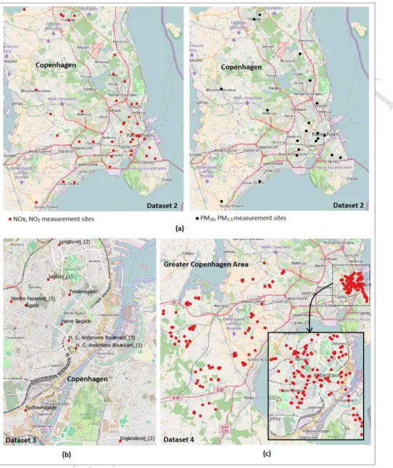
research work. In this study, new AirGIS has been evaluated against four measurements datasets (see 112

chapter 2.4 for further details and references to the datasets): (1) several years of long-term 113

measurements (1994 – 2015) from four permanent monitoring stations of the Danish air quality 114

1 _{See: https://www.postgresql.org/} 2 _{See: https://postgis.net/}

M

AN

US

CR

IP

T

AC

CE

PT

ED

10), (3) another set of 5-week passive measurements along ten major streets in Copenhagen, Denmark 116

(2011), (4) 1-month measurements campaign at the 204 addresses in Greater Copenhagen area, 117

Denmark (1994-5). The new model’s performance is assessed by taking into account different temporal 118

(single location, annual, daily averages etc. of concentrations) (dataset 1, 2, 4) and spatial (several 119

locations, single time interval) (dataset 2, 3, 4) variations of air pollution levels under varying urban 120

settings representing a wide range of traffic patterns and street geometries. As compared to the 121

previous validation study (Ketzel et al., 2011); this research work differs mainly in pollutants included, as 122

also PM10 and PM2.5 have been included in the new model evaluation. 123

2. Materials and methods 124

2.1 The AirGIS system 125

This section summarizes the general working principle of the AirGIS modelling system. 126

AirGIS (http://envs.au.dk/en/knowledge/air/models/airgis/), is part of the multiscale integrated 127

dispersion modelling system THOR4 covering coupled modelling of regional background concentration , 128

urban background concentrations and street concentrations (Brandt et al., 2001). Based on national GIS 129

datasets, AirGIS generates input files for the street pollution model OSPM® to estimate air pollution at 130

address locations. Automatic generation of necessary input files (traffic and street geometry information 131

etc.) for OSPM, is one of the key features of AirGIS that would otherwise be very tedious and time 132

consuming to produce for a large number of addresses. This, consequently, enables estimation of air 133

quality levels at a large number of addresses in an automatic and effective way. AirGIS is able to 134

estimate air pollution at any address location in Denmark. In the case that the address is located along 135

minor roads (<=500 veh/day) only the urban background concentration is assigned. In case the address 136

is located near a road with significant traffic (>500 veh/day) the street pollution model OSPM is applied 137

additionally to the urban background. The air pollution concentration is modelled at a receptor point 138

close to the building façade in a standard height of 2m, but it is possible to change the receptor height 139

e.g. in case of available information about the floor number of addresses in a multi-floor apartment 140

building. 141

The AirGIS system operates at three different levels of pollution (Figure 1). The working principle of 142

these three dispersion models is summarized as follows: (1) The Danish Eulerian Hemispheric Model 143

(DEHM) (Christensen, 1997) calculates the regional background concentrations in a 5.6 km x 5.6 km grid 144

resolution. It is a three dimensional, offline, large-scale, Eulerian, nested grid (Denmark: 5.6 km x 5.6 km, 145

Northern Europe: 17 km x 17 km etc.), atmospheric CTM model developed to study long-range transport 146

of air pollution on the Northern Hemisphere. DEHM includes emissions from all sources outside the area 147

including traffic, small-scale combustion, power plants, industrial units etc. using a comprehensive 148

chemical scheme based on photochemistry and particles (Brandt et al., 2012) (2) The Urban Background 149

Model (UBM) (Berkowicz, 2000b) calculates the urban background concentrations in a 1 km x 1 km grid 150

M

AN

US

CR

IP

T

AC

CE

PT

ED

linear approach for vertical dispersion up to the boundary layer. (3) The Operational Street Pollution 152

Model (OSPM)5 _{(Berkowicz, 2000a; Kakosimos et al., 2010) calculates the street contributions where} 153

background concentrations from DEHM/UBM are included via AirGIS system. OSPM® uses a 154

combination of a plume model for the direct contribution from the traffic source and a box model for 155

the recirculating part of the pollutants inside the street canyon environment. While adding contributions 156

from three pollution levels, NOx-NO2 non-linearity is taken into account in all models by a full 157

atmospheric chemistry module in DEHM and simple NO-NO2-O3 chemistry modules in UBM and OSPM 158

models. 159

The emissions database for Denmark has a high spatial resolution of 1 km x 1km and is based on SPREAD 160

methodology (Plejdrup and Gyldenkærne, 2011) for the spatial distribution of national emissions. In the 161

current model system, meteorological datasets (wind speed, wind direction, air temperature etc.) that 162

are used as input to all models (DEHM, UBM, OSPM) are based on WRF model (NCAR, 2018). Moreover, 163

regional background concentrations that are input to UBM are considered as spatially homogenous over 164

the city and nearby surroundings. While treating background concentrations, it is important that a 165

double counting of emissions should be avoided (Lefebvre et al., 2017). In our model chain, UBM takes 166

DEHM concentrations 25 km upwind (hour by hour depending on wind direction) and models only 167

emission of the closest 25 km – thereby avoiding double counting of emissions. Then, OSPM calculates 168

the “street increment”, considering only the contribution of the closest street to the address, on top of 169

the UBM background (1km x 1km horizontal resolution) not introducing double counting either. 170

171

Figure 1: An illustration of the spatial variation of three air pollution levels considered in the AirGIS system. DEHM: 172

the Danish Eulerian Hemispheric Model; UBM: Urban Background Model; OSPM: Operation Street Pollution 173

Model; Light green colour indicates the level of regional background concentrations; Yellow colour indicates the 174

urban background concentrations; Maroon colour indicates the direct street contributions (traffic hotspots). 175

M

AN

US

CR

IP

T

AC

CE

PT

ED

concentrations are averaged over the time period corresponding to those used in the exposure studies. 177

This allows a calculation of short-term and long-term averages of air pollution estimates which can be 178

beneficial for health related studies based on exposure assessment at street level. Furthermore, the 179

modelling system has been through continuous refinement i.e. in context of input datasets on traffic 180

and street geometry, vehicle emission factors, chemistry etc. (e.g. Ketzel et al., 2012). Recently, the 181

system has been extended to and validated for PM10, PM2.5 and BC (Hvidtfeldt et al., 2018). At present, 182

the complete modelling system allows for the estimation of various air pollutants including NO2, NOx, 183

PM10, PM2.5, CO, O3 and BC. 184

2.2 New AirGIS architecture 185

This section summarizes the new features and updates in the AirGIS system. In addition, similarities and 186

differences in the two systems (old and new AirGIS) have also been highlighted. 187

2.2.1 New system overview 188

An overall overview of the new AirGIS is as follows. Unlike the former AirGIS, the new model system 189

makes use of open-source GIS programming tools in PostgreSQL software, with GIS functions provided 190

by its spatial extension i.e. PostGIS, in conjunction with R scripting language (The R Core Team, 2017) 191

interface for pre- and post-processing of the datasets. The processing speed for spatial operations in 192

PostGIS is greater than for other common desktop GIS applications due to its efficient use of spatial 193

indexing (Gulliver et al., 2015). This is of particular importance for the application of new AirGIS that 194

uses address points with exposure periods, road networks with traffic composition information and 195

buildings footprints with building heights information as input for a large geographical region of interest. 196

As such, PostGIS provides an effective environment in which to handle these large spatial data sets. R 197

scripts (via R-Studio) provide a seamless interface to query data from PostgreSQL database as well as to 198

execute PostGIS commands. The main aim of using R software has been (1) to strengthen the new 199

system by its significant statistical computing capabilities (2) to perform preliminary data analyses as 200

soon as PostGIS commands execution is completed (3) to provide a single flexible environment to 201

perform all data handling from pre-processing via running GIS queries to post-processing and export to 202

OSPM and UBM model runs. Following sub-sections summarize the working principle of the new model 203

system as well as briefly compare it with the former AirGIS. 204

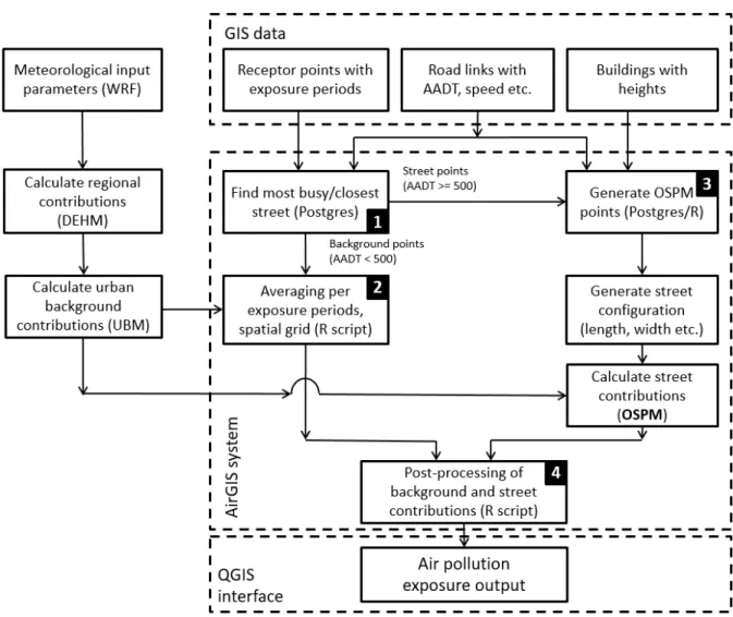
Figure 2 shows an overall structure and dataflow of the new AirGIS and is explained in the following. 205

M

AN

US

CR

IP

T

AC

CE

PT

ED

Figure 2: An overall structure and dataflow of new AirGIS architecture. See also list of abbreviation at the 208

beginning of the paper; Block GIS data represents the input GIS shapefiles (receptors points, road networks, 209

building footprints); Block AirGIS systemrepresents the new AirGIS processing workflow, numbered boxes indicate 210

the key steps of workflow, see text; Block QGIS interface represents the visualization interface to view/assess air 211

pollution exposure output. 212

Block GIS data (Figure 2) represents the spatial input data i.e. address points (with exposure periods),

213

road networks (with traffic information) and building footprints (with building heights). Traffic 214

information includes annual average daily traffic (AADT) flow for passenger cars, vans, lorries and buses 215

and the travel speed for varying vehicle categories for each street. The input files are stored in a 216

PostgreSQL/PostGIS database for the geometric processing. 217

Block AirGIS System (Figure 2) represents the central part of new AirGIS workflow. In this block, first, the 218

closest/most busy street to each address location within a certain buffer distance (e.g. 30m – 50m, the 219

empirical radii and easy to change by the user) are searched (via Postgres script) (Figure 2, “step 1”). 220

During this search, the address points are divided on the basis of AADT value at the closest/most busy 221

street into two categories i.e. urban background point (hereafter, background point) and street 222

M

AN

US

CR

IP

T

AC

CE

PT

ED

and changeable), then the street contribution (calculated by OSPM) is usually very small and can be 224

neglected. Therefore, such address points are assigned as background points (bypassing the OSPM 225

calculations). Otherwise, the address points are assigned as street points. 226

Concerning the background points, they are processed only in connection to the urban background 227

contributions. The coupled models chain works as follows: WRF provides meteorological input to DEHM 228

model to estimating regional background concentrations that are input to the UBM model (Figure 2). 229

The urban background concentrations are calculated with the UBM model and, subsequently, averaged 230

according to the exposure periods and spatial grid, via R script (Figure 2, “step 2”). Thus, in the new 231

system, transport and chemistry of pollutants are generally treated in the same way as the former 232

system. Here, it should be noted that the previous versions of AirGIS, sometimes, also made use of (i) 233

regional/background monitoring data as background concentrations (depending on the availability) (ii) 234

simplified SUB method (Berkowicz, 2000b) to estimate urban background pollution levels. Presently, in 235

the new system, background-monitoring data is only used to validate overall model output. 236

Furthermore, only DEHM and UBM are used to estimate background concentrations. 237

After estimation of background concentrations (Figure 2, “step 2”), the new system processes the street 238

points (AADT >= 500). That is, new AirGIS via an automatic Postgres script, generates for each address 239

point an orthogonally projected point on the closest street centerline (referred as OSPM points) (Figure 240

2, “step 3”). Once OSPM points are generated, the new system produces the street configuration 241

information (street width, lengths etc.) for each of these points. The process of generation of street 242

configuration in the new system is described in detail in the sub-section 2.2.2. 243

Once street configuration is generated, the input files for OSPM calculations in the required format are 244

produced. Hereafter, OSPM runs take place to calculate street contributions. Then, OSPM’s output 245

together with DEHM/UBM results is further processed through R-scripts (post-processing) (Figure 2, 246

“step 4”) to produce exposure output. This is one of the unique innovative features of the new AirGIS 247

where pre- and post-processing is handled via R scripting interface enabling processing of large datasets. 248

In the former AirGIS system, pre- and post-processing was handled in a number of manual steps. 249

Finally, block QGIS6 interface (Figure 2) (QGIS Development Team, 2018) represents the visualization

250

interface during the whole modelling process, where both input and output files can be visualized 251

readily in a direct link to the Postgres database. 252

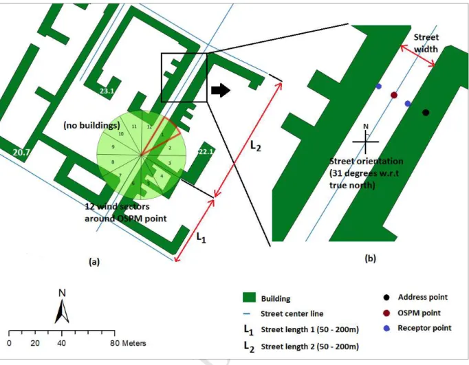
2.2.2 Computation of street configuration 253

Here, in this section, the process of estimation of street configuration in the new system is summarized. 254

We recall that for each OSPM point (residing on street center line), the new model system generates 255

street configuration information by making use of scripts written in PostGIS programming environment 256

and streets and buildings spatial data sets. The street configuration information, in general, represents 257

M

AN

US

CR

IP

T

AC

CE

PT

ED

sectors) around the receptor points (ii) static data that will be produced only once for each address 259

location. 260

Similar to the former AirGIS (Jensen et al., 2001), the new model system uses the concept of 2½ 261

dimensional urban landscape model (Hansen et al., 1997) to estimate street configuration information 262

for each OSPM point. The term “2½ dimensional” (also known as pseudo-3D) describes the 2D graphical 263

projections to appear as three-dimensional (3D), when in fact they are not (Wikipedia, 2018). Thus, the 264

estimated street configuration information (street orientation, street lengths etc.) of the both systems, 265

due to the same concept, is essentially similar to each other with only difference that is, in the new 266

system it is implemented (“re-programmed”) in a new language, here PostGIS. 267

The procedure of street configuration estimation is as follows. For each OSPM point (located at street 268

center line), the new system first estimates the street orientation. The street orientation (00 _{– 180}0_{) is} 269

usually computed clockwise according to the true north (Figure 3b) and determined by computing the 270

direction of the street center line nearest to the receptor point. Based on this concept, the PostGIS 271

script in the new system, first splits the road network shapefile (multilinestring) into individual line 272

segments (linestring), and then the nearest line segment (edge) is used to estimate the street 273

orientation. 274

Air pollution levels are influenced by the buildings layout in a street canyon environment (Vardoulakis et 275

al., 2003; Xie et al., 2005; Shu et al., 2014). The new model system handles this phenomenon in the 276

same way as the old system. The system creates 12 wind sectors, where each wind sector covers an 277

angle of 30 degrees. Based on above criteria, new AirGIS generates wind sectors around OSPM point to 278

estimate the height of the buildings in wind sectors (Figure 3a). First, the new system generates 12 wind 279

sectors within 50m buffer (changeable) around each OSPM point (Step 1). Then, the first wind sector pie 280

is aligned to the street orientation (Step 2) and subsequently it is used to locate the building as well as to 281

identify the associated building height of that wind sector (Step 3). Furthermore, the new model also 282

searches for the general building height i.e. the most prevalent height among wind sectors. If the 283

prevalent height is zero, the general building height is estimated as zero, which is allowed and handled 284

appropriately in OSPM. 285

M

AN

US

CR

IP

T

AC

CE

PT

ED

Figure 3: A representative scenario of street configuration estimation in the new AirGIS via PostGIS scripts 287

(visualization in QGIS software) (a) the generation of 12 wind sectors (with first wind sector aligned to the street 288

orientation) to estimate the height of the buildings in wind sectors. Sectors 9 and 10 are the examples of “no 289

buildings” case. Buildings heights (in meters) and examples of street lengths (length 1 and 2) have also been 290

shown. The minimum and maximum allowable lengths are 50m and 200m, respectively (b) the example of street 291

configuration parameters (width, orientation) in the new AirGIS system. Address point, OSPM point and receptor 292

point have also been shown. 293

Next, the new system computes the street length, as distance from OSPM point to the nearest street 294

intersections on both sides. Based on empirical values, the minimum allowed street length is 50m and 295

the maximum allowed street length is 200m. 296

Among street configuration parameters, street width has a key importance. The new model system 297

estimates the street width (Figure 3b) as follows. First, the new system finds the intersection of 50m 298

buffer around the OSPM point and the nearest building polygons on each side of the street. Based on 299

this intersection, the new model generates parallel lines on both sides of the street aligned with closest 300

buildings. Then, distance from OSPM point to the parallel lines is calculated and summed as the 301

estimated street width. This approach also works when there are buildings on only one side of the 302

street. A brief comparison of former and new AirGIS systems (Figure S1, S2, S3 and Table S1), in terms of 303

M

AN

US

CR

IP

T

AC

CE

PT

ED

304

material. The comparison shows a good agreement between estimated street configuration of the old 305

and new systems. Furthermore, to summarize, Table 1 lists similarities and differences in the former and 306

new AirGIS systems. 307

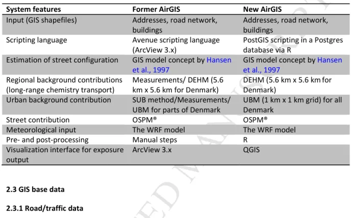
Table 1: List of similarities and differences in the former and new AirGIS systems. 308

System features Former AirGIS New AirGIS

Input (GIS shapefiles) Addresses, road network, buildings

Addresses, road network, buildings

Scripting language Avenue scripting language (ArcView 3.x)

PostGIS scripting in a Postgres database via R

Estimation of street configuration GIS model concept by Hansen et al., 1997

GIS model concept by Hansen et al., 1997

Regional background contributions (long-range chemistry transport)

Measurements/ DEHM (5.6 km x 5.6 km for Denmark)

DEHM (5.6 km x 5.6 kmfor Denmark)

Urban background contribution SUB method/Measurements/ UBM for parts of Denmark

UBM (1 km x 1 km grid) for all Denmark

Street contribution OSPM® OSPM®

Meteorological input The WRF model The WRF model

Pre- and post-processing Manual steps R

Visualization interface for exposure output

ArcView 3.x QGIS

309

2.3 GIS base data 310

2.3.1 Road/traffic data 311

Road traffic data sets have a key importance for modelling traffic air pollution. In Denmark, road traffic 312

information is based on a national traffic database in form of a GIS shapefile. The GIS road network is 313

originally based on the TOP10DK road network of the National Survey and Cadastre from 1999 that was 314

subsequently updated to KORT10 road network i.e. the nationwide object-oriented map, since 2007 315

(https://kortforsyningen.dk/indhold/data , Jensen et al., 2009a). The digital mapping of the roads is 316

based on aerial photos (spatial resolution: 40 cm x 40 cm) and precision is high (about 1m) for the center 317

line of the road (The Danish Geodata Agency, 2006). The traffic database, therefore, contains polyline 318

shapes representing the road center line and a list of relevant traffic related attributes that are required 319

for the geometric processing in new AirGIS, and later OSPM. The most relevant attributes of the GIS 320

road network are road type (to specify street type, see Table 2), AADT, and travel speed (Jensen et al., 321

2009b). 322

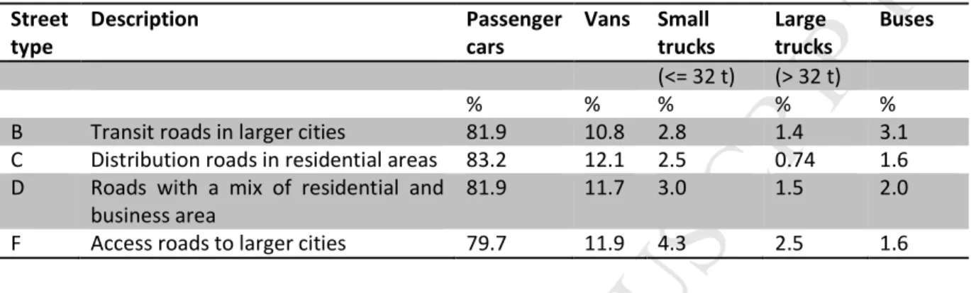
The street type specifies the vehicle distribution and the diurnal variation in traffic, the so-called OSPM 323

street types. Table 2 shows an overview of the street classification used in the AirGIS system. Each 324

OSPM street type refers to a text file containing information about hourly traffic distribution for 325

different days and vehicle types (passenger cars, vans, small and large trucks, buses). Days include 326

Monday – Thursday, Friday, Saturday, Sunday and further divided on the month of July (summer 327

M

AN

US

CR

IP

T

AC

CE

PT

ED

each vehicle category and arbitrary hour of the year, required to calculate air pollution concentration. 329

See Jensen et al., (2009a) for further details and an example of OSPM street “type B”. 330

Table 2: The street classification used in the AirGIS modelling system to estimate air pollution concentrations 331

(using OSPM) at any address location in Denmark (source: Jensen et al., 2009a). 332 Street type Description Passenger cars Vans Small trucks Large trucks Buses (<= 32 t) (> 32 t) % % % % %

B Transit roads in larger cities 81.9 10.8 2.8 1.4 3.1

C Distribution roads in residential areas 83.2 12.1 2.5 0.74 1.6 D Roads with a mix of residential and

business area

81.9 11.7 3.0 1.5 2.0

F Access roads to larger cities 79.7 11.9 4.3 2.5 1.6

333

Furthermore, in addition to the above mentioned national/Danish datasets, several open-source GIS 334

data of road links, buildings and address points are also available and useful when applying AirGIS 335

outside Denmark, see Table S2 (Appendix B, supplementary material).

336

2.3.2 Building data 337

Information on building foot prints as polygon shapefile is also available for the whole of Denmark based 338

on a national data set (Kort10 DK) obtained from the Danish Geodata Agency (http://gst.dk). Building 339

height was estimated for each building based on the National Elevation Model that has a resolution of 340

1m x 1m calculated as the difference between DTM (Danish Terrain Model) and DSM (Danish Surface 341

Model). 342

2.3.3 Address point data 343

Geocoded address locations (point data) are available for the whole Denmark via the Central Person 344

Registry. For smooth processing of the new AirGIS algorithms, it is important that an address point 345

should be inside building polygon. The address locations are assigned with exposure periods, which can 346

be short-term and/or long-term as per population exposure study design. The receptor point is usually 347

assumed to be at 2m height as standard and near the façade of the building closest to the address point 348

or curbside of the street in case of no building. However, other heights can be modelled when 349

information about height is available, e.g. floor number of an apartment. 350

2.4 Measured air pollution datasets 351

Model evaluation is indispensable for reliable air pollution exposure estimates. The new AirGIS 352

modelling system has been evaluated against various available measurements datasets (Table 3). In 353

addition, measurements of the Danish Air Quality Monitoring Programme (dataset 1) have also been 354

used to calibrate the new modelling system in terms of modelled PM (see chapter 2.5). 355

M

AN

US

CR

IP

T

AC

CE

PT

ED

modelling system. 357

Dataset Name Pollutant Measurement site Measureme nt method Time resolution Location (city) Time Period 1 Danish Air Quality Monitoring Programme (NOVANA) NOx, NO2, PM10, PM2.5 4 permanent kerbside Active/ continuous Hourly Copenhage n, Odense, Aarhus, Aalborg 1994 - 2015 2 ESCAPE-EU Danish campaign NOx, NO2, PM10, PM2.5 41 streets (20 streets for PM) Passive, active 3 obs./ 14 days Greater Copenhage n area November 2009 – October 2010 3 Five weeks passive sampling campaign NO2 10 major streets Passive 1 obs./ 5 weeks Copenhage n October 24 – November 28, 2011 4 1-month campaign

NO2 204 addresses Passive 6 obs./ 1

month Greater Copenhage n area 1994 - 1995 358

Figure 4 shows the locations of measurement sites of datasets 2, 3 and 4 in Copenhagen, Denmark and 359

Figure S4 (Appendix C, supplementary material) shows locations for dataset 1. The following sub-360

sections summarize various measured air pollution datasets. 361

2.4.1 Dataset 1 – The Danish Air Quality Monitoring Network 362

The urban part of the Danish Air Quality Monitoring Network consists of five permanent kerbside 363

stations in four major cities of Denmark (see: http://envs.au.dk/en/knowledge/air/monitoring/, for 364

more details; Ellermann et al., 2018). All stations monitors provide hourly measurements of various 365

pollutants (NOx, NO2 etc.) Among five permanent stations, the street station in Odense, Denmark has 366

been moved to the new location i.e. Grønløkkevej (ODGR), and has only been operational since 2015. 367

However, measured data at the previous location i.e. Albanigade (ODAL) was available. Furthermore, at 368

H.C. Andersens Boulevard (HCAB) monitoring station in Copenhagen, Denmark, there was a change in 369

street layout in 2010 that moved traffic closer to the station (Ellermann et al., 2018). Consequently, this 370

led to the lack of reliable historic measured data (e.g. year 2010) at HCAB. In turn, HCAB was excluded 371

from the analyses. Thus, in this study, long-term series (22 years) of half-hourly measurements at four 372

permanent street stations i.e. Jagtvej (JGTV) in Copenhagen, Albanigade (ODAL) in Odense (old location), 373

Banegårdsgade (AARH) in Aarhus, and Vesterbro (AALB) in Aalborg, are used to evaluate the new model 374

performance. For the new model evaluation, we used measured concentrations (µg/m3_{) of NOx, NO} 2, 375

PM10 and PM2.5 in the years 1994-2015. 376

2.4.2 Dataset 2 – Danish measurement campaign within ESCAPE project 377

M

AN

US

CR

IP

T

AC

CE

PT

ED

(http://www.escapeproject.eu/, Eeftens et al., 2012), in which 20 study areas across Europe were 379

included to investigate the spatial variation of particles and nitrogen oxide (NOx). The Danish 380

measurement campaigns (Figure 4a) were conducted from November 2009 to October 2010 and 381

covered 41 sites near Copenhagen for the measurements of NOx, NO2 and 20 sites for the 382

measurements of PM10 and PM2.5. A 14-days measurement campaign was conducted three times for 383

each site (N=41 sites for NOx, NO2; N=20 for PM). Failed measurements were repeated later to have 384

three valid observed values. Further details about measurement campaign and samplers used are 385

provided in Eeftens et al., (2012). 386

2.4.3 Dataset 3 – NO2 2011 measurement campaign

387

In order to evaluate the performance of AirGIS/OSPM for more locations in addition to permanent sites 388

(Dataset 1), a 5-weeks passive measurement campaign was performed to measure NO2 concentrations 389

(in µg/m3_{) along ten busy roads (Figure 4b) in Copenhagen, Denmark from October 24}th_{, 2011 to} 390

November 28th, 2011 (The FORCE Technology, 2018). The measurements were conducted using passive 391

samplers by IVL, Gothenburg, Sweden (Ferm & Svanberg, 1998) that were mounted at lamp posts, traffic 392

signs or building façade in about 2m height. This dataset was also used previously to validate former 393

AirGIS/OSPM (Ketzel et al., 2012). 394

2.4.4 Dataset 4 – NO2 measurement campaign at the 204 addresses

395

Another dataset from a comprehensive measurement campaign at the 204 addresses was available 396

within the Childhood Cancer project (see Raaschou-Nielsen et al., 2000 for more details). Measurement 397

campaigns were conducted at 103 street locations in the central Copenhagen, Denmark, and 101 398

locations in the Greater Copenhagen Area (20 – 50 km outside). Seven measurement campaigns 399

covering 30 locations took place in October – November 1994 and in April – June 1995. At each 400

measurement site, monthly mean concentrations of NO2 were measured for six consecutive months 401

(N=1224). Passive samplers were placed about 0.5m from the building façade and 4m above street level. 402

M

AN

US

CR

IP

T

AC

CE

PT

ED

Figure 4: Locations of various measured datasets used to evaluate the performance of New AirGIS modelling 404

system (a) Dataset 2 – the ESCAPE project measurement sites (NOx, NO2: 41 sites, PM: 20 sites) in the Greater

405

Copenhagen Area during November 2009 – October 2010 (b) Dataset 3 – locations of the 10 measuring points 406

(NO2) along major roads in Copenhagen using passive samplers during October 24th, 2011 to November 28th, 2011

407

(c) Dataset 4 – NO2 measurement sites at the 204 addresses in the Greater Copenhagen Area during October –

408

November 1994 and April – June 1995. 409

2.5 PM calibration and model evaluation statistics 410

The modelling of PM concentrations is still under development within the AirGIS system and new 411

components of the PM mass have recently been added e.g. secondary organic aerosol (SOA) in DEHM. 412

However a comparison of modelled PM10 and PM2.5 concentrations against measurements using the EU-413

reference method to determine PM at the permanent stations of the Danish Air Quality Monitoring 414

M

AN

US

CR

IP

T

AC

CE

PT

ED

reason for this is most likely a remaining underestimation for some of the PM constituents in DEHM 416

such as primary organic PM, secondary aerosols or water content in PM, and underestimation in OSPM 417

of non-exhaust from traffic (road wear, tyre wear and brake wear). In order to compensate for the 418

underestimation by the model we applied correction factors of 1.46 and 1.26 to all our modelled 419

concentrations of PM10 and PM2.5 values in this study. However, no calibration factors were applied to 420

the modelled NOx and NO2. 421

Model performance is often evaluated on the mixture of spatial (several locations in space, only one 422

time average) and temporal (one single location, timer series of many measurements e.g. annual, daily 423

etc.) variation of predicted values. In our modelling system, the temporal variation of the modelled 424

values evaluates mainly the whole chain of air pollution dispersion models (DEHM/UBM/OSPM) but to 425

less extent the GIS part. While the spatial variation of modelled values reflects the performance of the 426

whole AirGIS modelling system and the correctness of the input data, e.g. building foot prints, 427

generation of street configurations or traffic data in the data base. 428

The performance of the new model system was primarily evaluated using spatial and temporal 429

correlations (Pearson’s correlation coefficient “r”). In addition, various other model evaluation statistics 430

i.e. the coefficient of variation (CoV), root mean-squared error (RMSE), normalized mean bias (NMB), 431

factor of two statistic (FAC2) (Carslaw, 2015) were also used (see Appendix D,supplementary material

432

for the definitions). All statistical analyses were performed in R version 3.4.0 (https://www.r-433

project.org/) using “OpenAir” R package (Carslaw and Ropkins, 2012). 434

3. Results and discussions 435

3.1 Model evaluation against measured dataset 1 436

3.1.1 Annual averages 437

This section presents the results of new AirGIS evaluation against measured dataset 1 with a set of 438

annual averages for various pollutants and for a large number of years (1994 – 2015). Thus, this part of 439

the model validation is mainly on temporal validation of the long-term trends. These trends in the model 440

are dominated by the trends in the emission data superimposed by year-to-year changes in the 441

meteorology i.e. variable average wind speed. 442

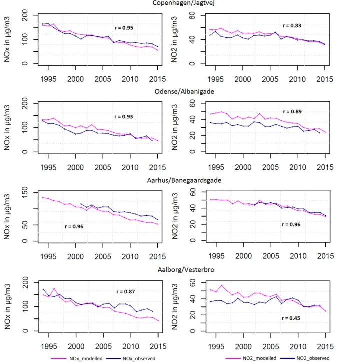
Results for several years of new model runs at four measurement stations i.e. JGTV, ODAL, AARH and 443

AARH are given as 22 years annual averages in Figure 5. For each station, trends for both NOx and NO2 444

are shown for modelled and observed street level concentrations (in µg/m3). A significant decrease in 445

NOx concentrations levels at all stations can clearly be observed, mainly caused by the changes in traffic 446

emissions (Ketzel et al., 2011). This trend is, in general, well reproduced by the new AirGIS over a 447

significant period of time. The changes in traffic emissions depend on traffic volume, vehicle distribution 448

(light and heavy duty vehicles, diesel versus gasoline) and vehicle specific emissions factors. Similar to 449

the former AirGIS system, long-term variation of emission factors is handled by the COPERT-IV model 450

(http://emisia.com/products/copert). Moreover, detailed information on changes in traffic volume or 451

M

AN

US

CR

IP

T

AC

CE

PT

ED

information might result in significant deviation between modelled and measured concentrations 453

considering single years. In this connection, more accurate traffic datasets based on systematic traffic 454

counts, have only been available since 2007 (Ellermann et al., 2018). 455

At all stations there seems to be a good match between measured and modelled values of NOx while 456

sometimes new model overestimated modelled values (e.g. for 1996 at ODAL) and underestimated 457

significantly at AARH and AALB stations (2009 – 2015). These discrepancies may be related to 458

uncertainties in the historic traffic and emissions datasets. As stated above, for the most recent years, 459

more reliable traffic and emissions datasets are available, as compared to more uncertain historic traffic 460

and emissions data. Therefore, historic traffic counts should be integrated into the new model system 461

when they are available. Correlation coefficients between 22 years annual average modelled and 462

measured values at these stations are found to be 0.95, 0.93, 0.96 and 0.87 respectively. These high 463

correlations indicate that new AirGIS reproduced well the long-term temporal trends of modelled NOx. 464

For NO2 the observed concentrations have been decreasing on all stations, over the past two decades 465

(Figure 5). In general, the long-term temporal NO2 trends are also well reproduced by the new modelling 466

system over a significant period of time (1994 – 2015). The new model, however, sometimes 467

overestimates and underestimates observed NO2 concentrations. In particular, new AirGIS 468

overestimates the observed NO2 values at JGTV, ODAL and AALB stations for the years 1995 – 2005. 469

Especially for the streets in Odense (ODAL) and Aalborg (AALB) the new model output seems to be 470

shifted by 10 – 13 µg/m3 and 14 – 18 µg/m3 respectively towards higher values. This significant 471

discrepancy, likewise NOx, may also be due to the uncertainties in historic traffic and emissions 472

inventory data. Furthermore, uncertainties in our model parameters, (e.g. the NO-NO2 reaction rate 473

chemistry), the fraction of direct NO2 emissions may also be the possible reasons for over-predicted 474

values. While, for the years 2010 – 2015, there is a good match between measured and observed NO2 475

values at all stations. In addition, a high correlation was found between 22 years annual average 476

modelled and measured NO2 concentrations at JGTV, ODAL and AARH stations with correlation 477

coefficients of 0.83, 0.89 and 0.96. While, for AALB station, the correlation coefficient was found to be 478

moderate i.e. 0.45, caused by the discrepancy before 2005. After 2005, the agreement at AALB is very 479

good. 480

M

AN

US

CR

IP

T

AC

CE

PT

ED

Figure 5: Annual averages trends for observed and modelled NOx (left column) and NO2 (right column) at four

482

urban street stations (measurements are part of the Danish air quality monitoring network; Ellermann et al., 2017), 483

dataset 1. 484

As noted above, in the previous validation study (Ketzel et al., 2011), the AirGIS system was not 485

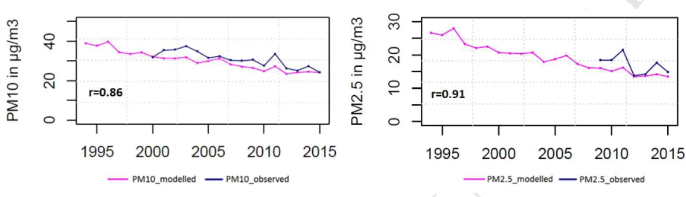
evaluated for PM10 and PM2.5. The performance of the new modelling system in reproducing long-term 486

trends (annual averages) of PM10 and PM2.5 is shown in Figure 6, however only for JGTV due to data 487

availability. The new model slightly under-predicted observed PM10 values for all the years with some 488

M

AN

US

CR

IP

T

AC

CE

PT

ED

emissions inventory data and inaccurate street configuration information. While, in terms of PM2.5 490

concentrations, the new model under-predicted observed value for all years except 2012 and 2013. 491

Despite these underestimations, the correlation coefficients between measured and modelled PM10 and 492

PM2.5 values were found to be 0.86 and 0.91, respectively. Thus, new AirGIS reproduced long-term 493

trends of PM10 and PM2.5 in a good agreement with the observed values at JGTV station. 494

495

Figure 6: Annual averages trends for the observed and modelled PM10 (left column) and PM2.5 (right column,

496

limited comparison due to the lack of measured data) at Jagtvej (JGTV) street station, dataset 1. Model results 497

include calibration see chapter 2.5. 498

3.1.2 Daily averages 499

For epidemiological research investigating health effects due to the short-term air pollution exposure 500

(e.g. Chen et al., 2018), the daily pollutants concentrations are used. Therefore the following sub-501

sections demonstrate the performance of the new model in reproducing the short-term temporal trends 502

(daily averages) of various air pollutants. As example, time periods for a recent year, 2015 and more 503

historic years 2005 and 2006 were selected. 504

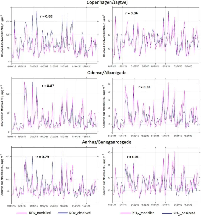
Year 2015 505

This section presents the results of new AirGIS evaluation against measured dataset 1 with a set of 4-506

months daily average air pollution levels during 1 January – 30 April 2015 for NOx and NO2. In terms of 507

PM10 and PM2.5, however, the new model evaluation is presented during 1 April – 31 July 2015 due to 508

data availability. 509

Table 4 presents the validation statistics on the daily averages (year 2015) of measured and predicted air 510

pollution. Figure 7 (left panel) shows the day-to-day variation of modelled and observed NOx (µg/m3_{) at} 511

JGTV, ODAL and AARH. Data at AALB was not available. At all stations, in general, there seems to be a 512

very good match between daily averages of modelled and measured NOx (Figure 7, left panel). This is 513

reflected by high positive correlation coefficients i.e. 0.88 (at JGTV), 0.87 (at ODAL) and 0.79 (at AARH), 514

respectively (Table 4). The new modelling system, however, sometimes over- and under-estimated the 515

observed NOx levels. At JGTV and AARH stations, for example, the under-estimations were in the range 516

10% – 27% (RMSE: 26.3 – 27.5 µg/m3_{) (Table 4).} 517

M

AN

US

CR

IP

T

AC

CE

PT

ED

modelled values (µg/m3) was observed. The correlation coefficients were found to be 0.84 (at JGTV), 519

0.81 (at ODAL) and 0.80 (at AARH), respectively (Table 4). In general, the new AirGIS reproduced well the 520

daily averages trends of modelled NO2. Nevertheless, in a few cases under- and over-estimations of 521

observed NO2 could also be seen. At all stations, RMSE was in the range 7.6 – 9.3 µg/m3 (Table 4). These 522

deviations are most likely related to uncertainty in the modelled day-to-day variation of local 523

meteorology (wind speed and direction, humidity, temperature etc.). In addition, uncertainties in the 524

representativeness of the urban background contributions may also be related to these discrepancies in 525

the new model output. 526

M

AN

US

CR

IP

T

AC

CE

PT

ED

Figure 7: Daily averages trends for the observed and modelled NOx (left column) and NO2 (right column) at four

528

urban street stations, dataset 1, during 1 January – 30 April 2015. 529

The data relating to the measured and modelled PM10 and PM2.5 are shown in Figure 8 for the street 530

station in Copenhagen (JGTV). Clearly, a very good agreement between daily averages (µg/m3_{) of} 531

modelled and measured PM10 as well as PM2.5 can be seen (Figure 8). This is depicted by high positive 532

correlation coefficients i.e. 0.84 (PM10) and 0.88 (PM2.5), respectively (RMSE: 2.9 – 4.2 µg/m3) (Table 4). 533

M

AN

US

CR

IP

T

AC

CE

PT

ED

Figure 8: Daily averages trends (during 1 April – 31 July 2015) for the observed and modelled PM10 (left column)

535

and PM2.5 (right column) at Jagtvej (JGTV) street station, dataset 1. Model results include calibration see chapter

536 2.5. 537

Table 4: Validation statistics for observed (obs.) versus modelled (mod.) concentrations (daily averages) of various 538

air pollutants (NOx, NO2, PM2.5, PM10) for dataset 1 in the year 2015. Av = average (µg/m3), FAC2= factor of two

539

statistic, NMB = normalized mean bias, RMSE = root mean squared error (µg/m3), R = Pearson’s correlation 540

coefficient. 541

Oxides of Nitrogen

NOx NO2

Station Method Av NMB FAC2 RMSE R Av NMB FAC2 RMSE R

JGTV obs. 70.3 31.9 mod. 52 -0.27 0.97 27.5 0.88 30.3 -0.05 0.99 7.6 0.84 ODAL obs. 31 17.9 mod. 33.2 0.08 0.87 13.7 0.87 19.3 0.08 0.90 7.9 0.81 AARH obs. 67.4 30.8 mod. 60 -0.10 0.94 26.3 0.79 30.3 -0.05 0.98 9.3 0.80 Particulate matter PM10 PM2.5

Station Method Av NMB FAC2 RMSE R Av NMB FAC2 RMSE R

JGTV obs. 20.1 11.4

mod. 19.5 -0.04 0.99 4.2 0.84 11.1 -0.02 0.98 2.9 0.88 542

Years 2005 and 2006 543

This section presents the results of new AirGIS evaluation against measured dataset 1 with a set of 4-544

months daily average air pollution levels during 1 January – 30 April 2006 (NOx, NO2), 1 April – 31 July 545

2005 (PM10) and 1 April – 31 July 2006 (PM2.5). 546

Table 5 presents the validation statistics on the daily averages (years 2005 and 2006) of measured and 547

predicted air pollution. Figure 9 (left panel) shows the observed and modelled NOx values (µg/m3_{) as} 548

daily averages, in the period 1 January – 30 April 2006 at JGTV, ODAL, AARH and AALB. The agreement 549

between measured and predicted NOx (µg/m3_{) seems to be quite good at street stations in Copenhagen} 550

M

AN

US

CR

IP

T

AC

CE

PT

ED

for the streets in Aalborg (AALB) and Aarhus (AARH), moderate (0.53) to slightly higher correlation (0.67) 552

(Table 5) was observed. Discrepancies in the new model output, in terms of over- and under-predictions, 553

could also be observed particularly at JGTV. For example, new AirGIS systematically under-predicted the 554

observed NOx at JGTV street station during 15 – 21 February and 20 – 27 April 2006. Moreover, 555

significant over-estimations (13%) of observed NOx values were found in the new model output at AARH 556

station (see NMB in Table 5). At AALB, there seems to be a significant discrepancy in the modelled NOx 557

(FAC2 = 0.64), and the new system under-estimated the observed NOx by 7%. One of the possible 558

reasons of these under- and over-estimations may be related to the uncertainty in the predicted 559

meteorology. Furthermore, it was noted above (see section 3.1.1) that more precise traffic datasets 560

based on systematic traffic counts, have only been available since 2007 (Ellermann et al., 2018). Thus, 561

uncertainty in traffic emissions can also be related to these significant errors in new modelling system 562

output. Similar uncertainties apply for the further pollutants and will not be repeated. 563

For the case of NO2 (Figure 9, right panel), correlation between modelled and measured values (µg/m3) 564

seems to be good (0.83) at street station in Odense (ODAL) (Table 5). For the street stations in 565

Copenhagen (JGTV) and Aarhus (AARH), correlation was found to be slightly higher i.e. 0.67 and 0.63. 566

While, moderate correlation (0.59) between the measured and modelled NO2 was observed at AALB 567

street station. RMSE, at all stations, was in the range 10.4 – 26.3 µg/m3 _{(Table 5).} 568

M

AN

US

CR

IP

T

AC

CE

PT

ED

Figure 9: Daily averages trends for observed and modelled NOx (left column) and NO2 (right column) at four urban

570

street stations, dataset 1, during 1 January – 30 April 2006. 571

Figure 10 shows the observed and modelled daily averages trends of PM10 (during 1 April – 31 July 2005) 572

and PM2.5 (during 1 April – 31 July 2006) at Jagtvej (JGTV) street station. In general, there is a good 573

M

AN

US

CR

IP

T

AC

CE

PT

ED

positive correlation coefficient r=0.79 (Table 5). In terms of PM2.5, a moderate correlation i.e. r=0.53 was 575

found between the measured and modelled values (µg/m3_{). Significant over- and under-estimations can} 576

clearly be seen (Figure 10) (Table 5) especially for the case of PM2.5, where NMB was found to be 0.31. 577

These discrepancies may be related to the uncertainties in the predicted meteorology and other factors, 578

as highlighted above. In general, these underlying uncertainties in the model (Figures 9, 10 and Table 5) 579

are a bit higher for older data (before ~2010) compared to more recent years. This might lead to slightly 580

higher uncertainty in the estimated historic air pollution exposure. 581

582

Figure 10: Daily averages trends for the observed and modelled PM10 (left column) (during 1 April – 31 July 2005)

583

and PM2.5 (right column) (during 1 April – 31 July 2006) at Jagtvej (JGTV) street station, dataset 1. Model results

584

include calibration see chapter 2.5. 585

Table 5: Validation statistics for observed (obs.) versus modelled (mod.) concentrations (daily averages) of various 586

air pollutants (NOx, NO2, PM2.5, PM10) for dataset 1 in the years 2005 and 2006. Av = average (µg/m3), FAC2= factor

587

of two statistic, NMB = normalized mean bias, RMSE = root mean squared error (µg/m3), R = Pearson’s correlation 588

coefficient. 589

Oxides of Nitrogen

NOx NO2

Station Method Av NMB FAC2 RMSE R Av NMB FAC2 RMSE R

JGTV obs. 129.9 57.1 mod. 104.9 -0.19 0.98 41.6 0.76 51.7 -0.09 0.99 14.1 0.67 ODAL obs. 87.4 36.9 mod. 75.5 -0.13 0.91 30.2 0.87 37.2 0.02 0.98 10.4 0.83 AARH obs. 120.3 49.6 mod. 134.8 0.13 0.91 52.8 0.67 56.8 0.16 0.96 17.9 0.63 AALB obs. 134.6 47.5 mod. 125 -0.07 0.64 117.9 0.53 49.5 0.05 0.90 26.3 0.59 Particulate matter PM10 PM2.5

Station Method Av NMB FAC2 RMSE R Av NMB FAC2 RMSE R

JGTV obs. 22.4 13.5

M

AN

US

CR

IP

T

AC

CE

PT

ED

590

This section presents the results of new AirGIS evaluation against the short-term measured dataset 2 as 591

part of the Danish measurements campaign in Copenhagen, Denmark (ESCAPE-EU project) conducted 592

from November 2009 to October 2010 for various pollutants (NOx, NO2, PM10, PM2.5). We present the 593

performance evaluation of the new modelling system in terms of reproducing both temporal and spatial 594

variation of the observed values. 595

In Table 6, we present the descriptive statistics on observed and modelled values of NOx, NO2, PM10 and 596

PM2.5.Figure 11 (a, b) shows the scatterplots of modelled NOx and NO2 (µg/m3) in terms of reproducing 597

temporal & spatial variation (3 sets of 14 days averages, N=123) of the observed values. There is a 598

considerable scatter in the modelled values of both NOx (Figure 11a) and NO2 (Figure 11b) as compared 599

to the measured ones. Furthermore, there seems to be a better agreement between measured and 600

modelled values of NO2 as compared to NOx. The correlation coefficients between modelled and 601

measured NOx and NO2 were found to be 0.74 and 0.73 (Table 6). Figure 12 (a, b) shows the scatterplots 602

of modelled NOx and NO2 (in µg/m3) in terms of spatial variation (average concentrations per site, N=41) 603

of the same observed values. Clearly, some scatter in the modelled values of NOx (Figure 12a) and NO2 604

(Figure 12b) and the deviation from one-to-one line can also be observed in this case. The correlation 605

coefficients in terms of reproducing spatial variation of observed NOx and NO2 were 0.79 and 0.81, 606

slightly higher than for the temporal & spatial variation. 607

Similarly, Figure 13 (a, b) shows the scatterplots of modelled PM10 and PM2.5 (µg/m3) in terms of 608

reproducing temporal & spatial variation (3 sets of 14 days averages, N=60) of the measured values. 609

Whereas, Figure 14 (a, b) shows the scatterplots of same pollutants in terms of reproducing spatial 610

variation (total average per site, N=20). The correlation coefficients between modelled and measured 611

PM10 and PM2.5 (µg/m3) (temporal & spatial variation) were found to be 0.74 and 0.80, respectively. In 612

terms of reproducing the spatial variation of observed PM10, PM2.5 values much lower correlations were 613

observed for PM10 (r=0.62) and PM2.5 (r=0.32). However, these correlations in terms of assessing spatial 614

variation of modelled PM are based on only 20 data points and therefore relatively uncertain and very 615

sensitive to single outliers. 616

For all compounds, the new model overestimates the concentrations compared to the observed values 617

by 25% to 71% (see NMB in Table 6). For NO2 and NOx the overestimation is quite large which is in 618

contrast to the overall comparison with dataset 1, where the agreement was much better. Cyrys et al., 619

(2012) in their work relating to the results of ESCAPE study compared Harvard Impactors samplers (NOx, 620

NO2) with the chemiluminescence method being the EU reference method. The authors reported 621

generally no to modest underestimation. Another companion paper (Eeftens et al., 2012) focusing on 622

PM observations revealed that the same kind of limited numbers of samplers were used to measure PM 623

during ESCAPE study. Interestingly, in Eeften’s work we noticed no such comparison to the EU reference 624

method in terms of the measured PM. However, Hvidtfeldt et al., (2018) in their work, compared the 625

Harvard Impactors used in the ESCAPE study with a high-quality fixed site monitoring instrument, SM200 626

(OPSIS Sweden, 2018), comparable to the EU reference method (Ellermann et al., 2018). The comparison 627