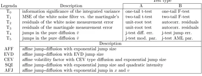
MPRA
Munich Personal RePEc Archive
Filtering and likelihood estimation of
latent factor jump-diffusions with an
application to stochastic volatility models
francesco paolo esposito and mark cummins
dublin city university, business school
1. May 2015
Online at
http://mpra.ub.uni-muenchen.de/64987/
Filtering and Likelihood Estimation of
Latent Factor Jump-Diusions with an
Application to Stochastic Volatility Models
F. P. Esposito
B
*and M. Cummins
B
**
DCU Business School
01/05/2015
Abstract
In this article we use a partial integral-dierential approach to construct and extend a non-linear lter to include jump components in the system state. We employ the enhanced lter to estimate the latent state of multivariate parametric jump-diusions. The devised procedure is exible and can be applied to non-ane diusions as well as to state dependent jump intensities and jump size distributions. The particular design of the system state can also provide an estimate of the jump times and sizes. With the same approch by which the lter has been devised, we implement an approximate likelihood for the parameter estimation of models of the jump-diusion class. In the development of the estimation function, we take particular care in designing a simplied algorithm for computing. The likelihood function is then characterised in the application to stochastic volatility models with jumps. In the empirical section we validate the proposed approach via Monte Carlo experiments. We deal with the volatility as an intrinsic latent factor, which is partially observable through the integrated variance, a new system state component that is introduced to increase the ltered information content, allowing a closer tracking of the latent volatility factor. Further, we analyse the structure of the measurement error, particularly in relation to the presence of jumps in the system. In connection to this, we detect and address an issue arising in the update equation, improving the system state estimate.
Keywords: latent state-variables, non-linear ltering, nite dierence method, multi-variate jump-diusions, likelihood estimation.
1 Introduction
The estimation of parametric models of stochastic dierential equations (SDE) has become a subject of growing interest in recent years, seeSørensen (2004), Aït-Sahalia (2006) for a survey. There are many approaches available, each designed to deal with specic problems connected to the inference exercise. It is dicult to classify the solution methods throughout the problems posed by the estimation of parametric SDEs. A partial categorisation discriminates by
Moment-based estimator. Seminal papers are the GMM of Hansen and Scheinkman (1995), the indirect inference of Gourieroux et al. (1993), the ecient method of moments of Gallant and Tauchen (1996) or the martingale estimating functions of Bibby and Sørensen (1995). Studies based on the characteristic function includeSingleton(2001),Chako and Viceira(2003).
Likelihood-based estimator. Seminal papers are the nite dierence approach as pioneered by Lo
(1988), the simulation of likelihood ofPedersen(1995a) or the Markov Chain Monte Carlo (MCMC) methods as independently derived byJones (1999), Elerian et al.(2001), Eraker (2001). Another interesting approach is the polynomial expansion as inAït-Sahalia(1999),Aït-Sahalia(2002), Aït-Sahalia(2008).
Comparison studies have been performed byJensen and Poulsen (2002),Lindström(2007),Hurn et al.
(2007) and in relation to ltering problems, see Lund (1997), Duee and Stanton (2012) and Christof-fersen et al.(2014).
The main issue with the estimation exercise is related to the fact that the likelihood of the stochastic model is generally not known in closed form, making the use of an exact likelihood estimator virtually impossible, except for a few limited special cases. A further problem is represented by the imperfect sample information about the system to be estimated. In the rst instance, the system is observed only at discrete times, which poses the problem of how to optimally project the system forward in time, given the current information. Secondly, problems of greater interest in nance involve the system state being only partially or indirectly observable, namely: stochastic volatility (e.g. Heston, 1993, Due et al.,
2000) and term structure models (e.g. Due and Kan,1996,Chen and Scott, 2003). This lack of infor-mation issue can be optimally solved by ltering, which basically consists of nding the mean square best estimate of the system state, given the partial set of historical information available. This can be viewed as a projection problem in the space of mean square integrable martingales, seeØksendal (2003). The whole ltering exercise boils down to the construction of the projection operator, jointly with an update procedure for the projection of the system state, once the observable information has been made available. Several authors develop ltering procedures to tackle the latency of the state components. Examples are
Bates(2006), Jiang and Oomen(2007). However, these algorithms are specic to an ane structure of the SDE and have in common the use of the spectral function for ane jump-diusion models, which is known in semi-analytical form (Due et al.,2000).
In this paper, we develop a particular of lter that can treat more general jump-diusion models and produce estimates of the state vector which include latent components. We then apply the lter within the context of a parametric model estimation. We acknowledge that a lter, similar in spirit to the one used here, has been recently applied to pure diusion models by Hurn et al.(2013). In that paper the authors apply the same procedure used in this article to derive the generic main ltering equation for non-linear pure diusions. They solve the nonlinearity problem via the application of a quasi-likelihood approach which is coherent with the estimation strategy they adopt. This paper is dierent in that we independently devise an extension to the non-linear lter which is able to handle multivariate jump components. The form of the jump is quite general, allowing the possibility to handle synchronous or asynchronous jumps, state-dependent jump size distribution along with ane as well as dierently specied state-dependent jump-intensities. The nonlinearity problem is solved with a second order ap-proximation which allows for a quasi-analytical form of the lter that can be implemented in a very exible fashion. Secondly, along the lines of the original approach found inMaybeck(1982), we comple-ment the lter with an estimation technique that adopts the same methodology used to derive the main ltering equation. The econometric procedure consists of an approximate maximum likelihood (AML) approach whereby the likelihood is obtained via the numerical solution of the partial integral-dierential equation (PIDE) describing the transition probability of the multivariate jump-diusion under analysis, with the application of the nite dierence method for the construction of the diusion operator and the use of a discretisation to deal with the jump component. Within the structuring of the main block of the approximated likelihood, we also discuss the issue of the stabilisation of the PIDE operator approxi-mation and report a criterion which provides a major guideline for this purpose. We also characterise in
ner detail the form of the general likelihood for the purpose of a simplied computer implementation. Finally, in the empirical section we analyse a stochastic volatility model with jumps with focus on the system state design. Inspired by previous works such asBollerslev and Zhou (2002), we introduce the integrated variance variable, which is proved to carry signicant auxiliary information when estimating the stochastic volatility factor. Moreover, we test the form of the measurement error variable, providing evidence that augmenting the state to model the error as an auxiliary latent system component is signif-icant. Along the lines ofDempster and Tang(2011) we provide evidence that a martingale form for the error is more desirable. Further, we have discovered that in the presence of jumps a pure diusion system state estimate might experience shocks that can be accommodated via the extension of the measurement error to jump components. Another interesting conclusion of this paper is that, depending on the system design, in the presence of jumps the measurement error might actually be a redundant system state com-ponent, whereby its impact on the system total variability is absorbed by the jump component projection. The paper is organised as follows. Section 2 presents the non-linear lter and as a key contribu-tion to the literature the extension of the ltering procedure for handling jump components. Seccontribu-tion 3 describes the estimation procedure and analyses the problem of the stabilisation of the PIDE operator approximation. Section 4 contains the empirical analysis of a suite of stochastic volatility models. It rst depicts the system equations used in the Monte Carlo simulation and further analyses from a statistical perspective the system design, with particular attention to the use of the integrated variance for the sake of the latent state estimation and the form of the measurement error as an auxiliary latent state variable. A further sub-section presents the estimation of the model parameters via AML and discusses some auxiliary measure of the lter performance. Section 5 concludes.
2 The construction of the nonlinear lter
The problem we tackle is the statistical estimation of a parametric model, which describes the dynamics of a vector-valued stochastic process(St)t∈[0,T). We callSt a system, essentially because the stochastic
dierential equations describing its components' dynamics are interconnected. The systemS is arranged
into two componentsS = (X, Y), in relation to their observability. We indicate the observable
compo-nents asY, whose dynamics are described as a function ofX, the state of the system. The system state X is fully or partially latent, that is its path can only be inferred from the information coming from the
measurementY. In solving the estimation problem, we are therefore concerned with the device estimating
the latent state of the system and with the construction of the full likelihood for parametric estimation purposes. This section is dedicated to the solution of the former problem, which, as a key contribution to the literature, is extended to include jump components. The construction of the likelihood is pursued in Section 3.
Filtering is the problem of nding the best estimate in a mean square sense of the state of the system, that is theGt-measurable random variableXt¯ that minimises the path-wise distance from the true state Xt. Let the probability space(Ω,F,Ft,P)and let the ow of information as represented by the setG ⊂ F,
be respectively dened as the algebra of events representing the observable trajectories and the full set of information about the system(X, Y). The solution to the problem dened above, is the projection
from the spaceL2(
P)onto the spaceK ⊂ L2(P)of theGt-measurable random variables. The projection
operator corresponds to the expectationE[·|Gt], see Øksendal (2003). The following aims to construct
an approximation of the projection operator, when the stochastic process is a jump-diusion. Actually, because the observables are recorded only at discrete times, we need two projection operators providing the latent state estimates. The approach undertaken here, following the cited seminal literature, consists of the derivation of two equations dening the operators of projectionE[Xt|Gt−δt]andE[Xt|Gt]. In order
to simplify notation, we will indistinctly indicateEt|s[X] =: E[Xt|Gs] := ¯Xt|s, s ≤t. Corresponding
to the previous expectations, the non-linear lter is composed of the following equations. The time-propagation equation moves the state estimates between the observation times t−δt and t, the time
segments being not necessarily equally spaced, whereas the update equation generates the new estimate of the partially latent state vector Xt when a new observation Yt is available. The update equation is
given in a convenient simplied form, as a function ofY and its projectionY¯, of the projected state vector
¯
X and their second order cross-moments. The problem amounts to the construction of the projection
and update operators of the rst two central moments of the system state. Formally, the framework is given by the parametric system state
dX =b(X−;θ)dt+A(X−;θ)dW +J(z;X−, θ)dN (1)
J depends on the mark pointz, whose distribution is parametric and may depend on the state. The
random drivers of the system are the Brownian vector W and the Poisson counting process N, with
stochastic intensityλ(X−;θ). The random functionsb, A andJ are assumed to satisfy conditions that
grant a unique solution for Eq. (1) (see e.g. Platen and Bruti-Liberati, 2010), ∀θ ∈ Θ. In Eq. (1)
we make explicit the dependency on the left limit ofX, that is its level immediately before the jump,
if any. Subsequently, this notation is dropped, whereby we focus on the construction of the estimation procedure. For a complete treatment of the stochastic integral X and its components, see, e.g., Cont and Tankov(2003),Hanson(2007). For the practical purpose of system estimation, we will assume that the jump size vector of the synchronous jump can be written asJ =G(z)f(X), with G= [gij(z)]ij and gij = 0when i 6=j, where f and g are mapping, respectively, from the domain of X and z, the mark
point vector, toR•. Here, the denition ofJ is a working tool which makes the jump size dependent at
the same time on the mark-point vectorz and on the stateX, but in a way that allows the factorisation
of the jump-component and the state component in the time-propagation equation. The functionsf and gincrease the exibility of the statistical model.
The forward equation
Later in the construction of the time-propagation operator, a key role is played by the Kolmogorov forward equation (KFE). In general, considering the SDE (1), the KFE that is the equation describing the transition probabilities of the system, is found as:
Proposition 2.1 (The multi-dimensional jump-diusion PIDE). The Kolmogorov forward equation for the Itô process with Poisson jump components (1) is
∂t [p] = (AX+JX) [p] (2)
where the dierential operatorAX is dened by the position,C=AA?
AX[p] ≡ 12 X ij ∂x2ixj[Cijp]− X i ∂xi[bip] (3)
and the integral operatorJX is dened as
JX[p]≡ −(λp) +
Z
Z
dQ(z;h)|∇h| (λp)◦h (4)
Proof. SeeHanson(2007)
In Eq. (4)Qis the jump size probability measure,h: X+→X− is the post-jump transform,|∇h|is
the determinant of the Jacobian ofhand we indicate by ◦the function composition operator. For ease
of presentation, we consider the counting process to be scalar and allow the synchronous jump vectorJ
to be state dependent or not. The jump intensity is the processλ(X).
The second component of the system is represented by the observation equation,
Y =qX(X) +E (5)
whereEis the measurement error, which is left unspecied at the moment. In Eq. (5) we assume a simple
linear form for q(X) = HX, through the constant matrix H. This case is relevant for the stochastic
volatility model, whereH is a pick matrix and for a latent factor term structure model, which targets
the estimation of the empirical measure. The extension of Eq. (5) to more general forms requires an approximation to be fully implemented, see e.g. Nielsen et al. (2000), Baadsgaard et al. (2000). See
Christoersen et al. (2014) for a study of non-linearity in the observation equation in the case of an unscented Kalman lter.
In this article, we need to include a further component to the system state. This auxiliary component, intrinsically latent by its nature, is a dening object of the jump component, that is its, possibly state dependent, intensity process. We give it here in its level eect form
λ=qλ(X) (6)
In the following we extend the time propagation equation as conceived byMaybeck (1982) to handle a marked point Poisson component, which can be state-dependent in the jump intensity function and in the jump size distribution. Our work relies on the intuition of using the jump operator of the forward equation to extend the system state projection dynamics to include a jump component and in deriving workable expressions for the estimation of the latent system-state. Furthermore, we also address from an implementation perspective a feature of the update equation arising when jumps are included in the system state equation and oer robust statistics conrming the eectiveness of the solution.
2.1 The time-propagation equation
In order to construct optimal estimates of the state of the system X, which is observed at discrete
times only, we need conditions for the evolution of the system state projections between two observation times. This is called the time-propagation equation. The idea in Maybeck (1982) is to derive possibly approximated ordinary dierential equations for the rst two moments ofX, cfr. Nielsen et al.(2000), Baadsgaard et al.(2000) d dtX¯ = R X∂tpdX d dtV¯ = R XX?∂ tpdX−ddtX¯X¯?−X¯ddtX¯? (7)
In Eq. (7), we substitute the KFE for the jump-diusion transition probability ∂tpto obtain an exact
or an appropriately proxied ordinary dierential equation (ODE) system forX¯
t|sandV¯t|s. The aim is to
calculate the solution of (7) for the jump-diusion (1). To obtain the solution the following integrals are involvedR
X(A+J)[p]andRXX?(A+J)[p]that because of linearity can be handled separately with
respect to each individual KFE operator. For the same reason, further synchronous jumps can be easily included to the state model. We split Eq. (7) into its diusion and jump component, using linearity of the operators, that is d
dt(·) =
d dt(·)A+
d
dt(·)J. To simplify notation, we indicate the operatorEP[·]with
(| · |)andEQ[·]withh| · |i. We nd that the diusion component of Eq. (7) is
Proposition 2.2 (The Diusion Component of the Time-Propagation Equation,Maybeck,1982).
d dt X¯ A = (|b|) d dt V¯ A = (|C|) + (|bX?|) + (|Xb?|)−(|b|) ¯X?−X¯(|b|)? (8)
Proof. See the Appendix.
The lter X,¯ V¯can be extended with the same approach described above, adapting the integration
procedure to handle the jump component. We derive the auxiliary lter component providing the following formal ODE system.
Proposition 2.3 (The Jump Component of the Time-Propagation Equation).
d dt X¯ J = h|G|i(|λf|) =:U d dt V¯ J = h|G|i(|λf X?|) + (|λXf?|)h|G|i+ (|λf f?|) h|gg?|i −UX¯?−XU¯ ? (9)
Proof. See the Appendix.
In the above, we have used the signto indicate component-wise multiplication. The jump component
(9) represents to the best of our knowledge a novel contribution to the literature and provides an extension to the nonlinear lter of Maybeck (1982) and the most recent applications in nance of Nielsen et al.
(2000), Baadsgaard et al. (2000) and Hurn et al. (2013), which can be used for the estimation of the latent state of jump-diusions. In order to get a workable expression to use for computations the time-propagation equations require the evaluation of the expectations on the RHS of the previous dierential expressions.
2.2 Approximating the expectation operator
With Eqs. (8) and (9), we have obtained an ordinary dierential system which describes the projection operators for the rst two central moments of the state-equation as a function of time. However, it has to be noticed that Eq. (8) and Eq. (9) are only a formal denition, because the RHS is in general unknown. In order to obtain a workable specication, we need to characterise this formal statement of the time-propagation equations. The approach undertaken in this paper is along the lines of the seminal papers cited above. The expectation of a generic scalar function of the stateq(X)is approximated by
taking a Taylor series expansion ofqaround the current state estimateX¯ and applying the operatorE[·],
to both side of the equation, cfr. Maybeck(1982),Nielsen et al.(2000), to obtain
E[q(X)] =q X¯+12trace
∇2q X¯
·V¯
+R, (10)
where we neglect the remainderR, which contains a third order central moment function. The truncated
second order expansion introduces bias correction and can be seen as a stochastic equivalent of the ex-tended Kalman lter1. It is interesting to notice that if the state functionq(X)is at most quadratic, the
1The extended Kalman lter corresponds to a rst order approximation within the same methodology, cfr., e.g.,Lund
expansion in Eq. (10) is exact. In general, we have obtained an estimate of the time-propagation equation for the jump diusion (1), with state-dependent jump intensities and amplitudes. This approach diers from that undertaken inHurn et al.(2013), which uses the quasi-likelihood to approximate the integral with numerical quadrature. We believe this approach oers convenience in allowing for the construction of the time-propagation equation for the estimation of the main projection operator in a quasi-analytical form and further it can be coded in a very exible fashion.
Example: state-independent ane jump-diusion
From Eqs. (8), (9) and (10) it is evident that when the b and λ are ane, the jump size is state
independent and the diusion matrix is at most a quadratic function of the state, the time propagation equations are exact and can even be solved explicitly. For instance, in the ane jump-diusion case, when the jump intensity isλ(X) =λ0+λ1·X and the synchronised jump vectorJ is state-independent,
we get the exact ODE system
d dtX¯ = a˜+ ˜BX¯ (11) d dtV¯ = D˜ + ˜BV¯ + ¯VB˜ ? where ˜ a = a+λ0 ˜ B = B+h|J|iλ? 1 ˜ D = AD2X¯A?+ (λ0+λ1·X¯)h|J J?|i
which admits a closed form solution. In other situations we have to revert to an approximated ODE. Example: non-ane volatility
When the stochastic system is not ane, we approximate the time-propagation equation via Eq. (10). In this example, we look at a scalar pure diusion, with an ane drifta+bX and a squared diusion
functionC=σ2X2γ, hence the ODE driving the system projection is then
d
dtX¯ = a+bX¯ (12)
d
dtV¯ = σ
2X¯2γ+σ2(2γ2−γ) ¯X2(γ−1)V¯ + 2bV¯
The expression (12) is used later within the experimental section, in junction with a larger system, when conducting an exercise with a non-ane model.
2.3 The update equation
The non-linear lter we have developed in the previous section has the purpose of projecting the system between two consecutive times, carrying over the whole set of information inferred by the observation vector for the sake of delivering the best estimate of the partially observed system state. Once the system is at the observation time tand new information is collected about Y, we need a means to incorporate
such quantities into the system state estimate in an optimal way. The update equation consists of a mechanism to estimate the expectation X¯
t|t by refreshing the system state projection with the newly
arrived informationYt+, which are the only observable quantities in the context of a latent system state.
The optimal lterX¯ represents the best estimate of the state under partial information, which is the
natural condition under which data on a phenomenon are presented to the researcher.
The update equation, fundamentally, consists of the application of Bayes' rule, when conditioning the state estimates onto the observed information set at current time. Assuming the update equation form is a linear function of the residuals, it can be found that:
Proposition 2.4 (The update of a linear projection, Maybeck, 1982). The update equation for the non-linear lter dened by Eqs. (8) and (9) is given by
¯ Xt|t = X¯t|s+ ΣxyΣ−yy1 Yt−Y¯t|s ¯ Vt|t = Vt¯|s−ΣxyΣ−yy1Σyx (13)
with Σyy = Et|s h Yt−Yt¯|s Yt−Yt¯|s ?i Σxy = Et|s h Xt−X¯t|s Yt−Y¯t|s ?i = Σ?yx
Proof. See the Appendix.
Embedding new information intoX¯
t|sabout the observed residualsYt−Y¯t|simports into the states
estimates information that would be lost otherwise.
For the application we construct in this study, the observation equation of interest is a linear function of the latent state,Y =HX where in generalH is a constant matrix. This assumption implies the exact
estimatesY¯ =HX¯,Σyy=HV H¯ ?. WheneverY is a generic function of the stateX,Y =q(X) +E, the
system variablesY¯, Σyy and Σxy are approximated via Eq. (10), cfr. Nielsen et al.(2000). We remark
that the update equation (13) in the general case of a nonlinear ltering corresponds to a rst order expansion of the projection operatorEt|t. Expanding this approximation to higher orders, whereby the
expectations are approximated via Eq. (10) is impossible.
2.4 The measurement error
In the observation equation (5), we left the measurement errorEunspecied. We discuss the modelling of
the processEin this section. In the literature the measurement error is generically indicated as a random
processEtwith zero mean and constant covariance matrixΣε, a white noise which is at most cross-section
correlated. However, in a recent paper, cfr. Dempster and Tang (2011), it has been statistically proved that the measurement error manifests mean reversion and cross correlation with the state. InDempster and Tang (2011), the authors plug the measurement error into the state equation, a choice that allows one to design an evolutionary equation forE that could better track the underlying state of the system X. The behaviour of the measurement error is actually the result of the ltering process, therefore it is
straightforward to expect a mean reverting or even a martingale behaviour which might have a random impulse which is correlated with the diusions W. The outcome of the inclusion of the measurement
error into the state vector consists of eectively transforming E into another latent component of an
augmented state vector. This is an implementation strategy that allows greater exibility in the system state ltering and the parametric estimation, introducing parameters that might be able to modulate the estimation residuals and improve the quality of the tting.
In this article we extend the intuition inDempster and Tang(2011) a step further. We report that in the presence of the jump component the measurement error can experience jumps that if neglected might propagate to the system state estimate and arise unexpectedly in other parts of the system. The case that we will be exploring in the empirical section is that of a latent pure diusion stochastic volatility whose ltered state, according to a certain measure to be specied, might sometimes experience excessive variations or jumps that can be improved or corrected by a measurement error that contemplates jumps. Thus, building on the same strategy, we will augment the system state by a measurement error vectorE
that, in general, will include a mean reversion term, a diusion and a jump component. However, having both a diusion and a jump component in the error term might result in a useless over-parametrisation. The general equation for the measurement errorE is
dE = (c+C0E) dt+C1dWE+JEdNE. (14)
We assume that the eigenvalues of the constant matrixC0grant that the processEis stationary or at least
non-explosive, whereas the constantcis such to compensate the drift generated by the jumpsΣNt
i=1Jti, if
any, and hence the unconditional mean is zero. As the vector processEbelongs to the system state, the
diusion component drivers might possibly be correlated with the diusive impulse ofX. The innovation
we introduce is to allow the measurement error to jump via the Poisson point process represented by the stochastic dierentialJEdNE. In general, the measurement error jumps may be synchronised or not
with theX component's jumps, whereby in the latter case an intensity function should be specied and
parametrised. However, we have found experimentally that at least for the model under test, the former case does not allow the exibility required to explain the unexpected jumps in the state estimate. When the measurement error jump processNE is not synchronised with the jump in the state, if any, a further
hypothesis on the dynamics of the stochastic intensity process should be specied. This may give rise to auxiliary latent measurement error variables. However, in the empirical section we will adopt the simplication that the jump error intensity is an ane function of the stateX. In several case studies,
3 Estimation
In Section 2 we have presented the procedure to estimate the system stateX in the presence of partial
information via a nonlinear lter, which has been extended to include jump elements. In this paragraph we complement that technique with an estimation method for the parametrisation of multivariate jump-diusions with latent components. Whereas we have exploited a PIDE approach for the derivation of the symbolic solution of the time-propagation equation (7) for the ltering of the latent stateX, here we use
an intrinsic ltering approach for the derivation of the likelihood function, whose main component is the solution of the PIDE which describes the transition probability density of the system (1). In treating the latter problem, we follow the route leading to the construction of the approximate likelihood function of the latent state by numerically solving the forward equation (2). We use an AML approach exploiting the inherent optimality properties of the exact likelihood that can be achieved asymptotically by the approximation, cfr. Pedersen (1995a), Poulsen(1999). The same result extends to the PIDE version, provided uniform convergence of the solution, seeLindström(2007). Finally, the approximate likelihood of the observed variableY is achieved via the numerical integration of the latent state component. The
contribution of this article in the estimation exercise involves a particular implementation strategy that allows further simplication of the AML algorithm. In the following we describe the approach under-taken in this paper in the development of the estimation algorithm, which allows a considerable saving of computational time. We also tackle the problem of the stabilisation of the PIDE operator approximation.
3.1 Approximate likelihood function
The objective is to build an approximate likelihood function for the observables, P(Yt|Yt−1), which is
able to capture higher order moments implied by the system probability structure. In order to handle the presence of the partially or totally latent system stateX, we use the classic Bayesian decomposition
of the full likelihood function, which is then concentrated onto the observable variable by marginalising the system state. The contribution of this article in the estimation problem is the characterisation of the likelihood function which hinges on the particular implementation strategy of the likelihood core componentP(Xt+1|Xt). As a result, we achieve a simplication of the estimation algorithm.
We work with the following equation:2
P(Xt+1|Yt)P(Yt|Yt−1) =
Z
dXtP(Xt+1|Xt)P(Yt|Xt)P(Xt|Yt−1) (15)
In Eq. (15) the likelihood component of the observables Y, that isP(Yt|Yt−1), acts as a normalisation
constant, hence it is obtained by integrating the RHS w.r.t. Xt+1. Furthermore, the above likelihood
function denes an iteration that recursively combines the transition probability of the system state with the density implied by the observation equation. The equation dened in (15) progressively generates the likelihood for the observables and the function P(Xt+1|Yt), which acts as a weighting function in
the successive step. The initial condition P(X0|Y−1) is set to
R
dX−1P(X0|X−1), wherever the initial
condition is not observable; otherwise, the initial condition is set to the observables.
In order to portray further the likelihood recursion, we exploit the solution chosen in the article of
Dempster and Tang(2011), by augmenting the system state with the measurement error, which renders the observation equation asY =qX(X). As a consequence we have thatP(Yt|Xt)≡δ[q(Xt)−Yt], where
δ is the pulse function. Concerning the latter statement, we need to clarify that we implicitly assume
that, whenever the observation function is not surjective, theY belongs to the image of q. Further, we
also notice that if any subcomponentXa of the partitionX = (Xa, Xb)does not enterqthen we simply
refer toP(Y|X) =P(Y|Xb)3.
To complete the construction of Eq. (15), we build its core component as the solution of the KFE via a combination of a nite dierence method (FDM) and an ordinary integral approximation. In re-cent years, the FDM has received renewed attention in continuous-time nancial econometrics, since the
2Equation (15) is obtained by plugging into the denition ofP(Xt+1|Yt) =R
dXtP(Xt+1|Xt)P(Xt|Yt)the probabilistic
correspondent of the update equation, that isP(Xt|Yt) = P
(Yt|Xt)P(Xt|Yt−1)
P(Yt|Yt−1) .
3However, if the range ofY does not coincide with the image ofq, the probabilityP(Y|X)would not be dened. In
fact, we have the chain of equalities
P(Y|Xa, Xb) = P(Xa
|Y,Xb)P(Y|Xb)
P(Xa|Xb)
and ifY /∈q(X), then {Y, Xb} ≡ ∅and P(Xa|Y, Xb)is not dened. Furthermore, from the RHS of the above chain we
seminal papers ofLo (1988), Pedersen (1995b) and Poulsen(1999). Examples areJensen and Poulsen
(2002),Lindström(2007),Hurn et al.(2010),Lux(2012).
We approximate each component P(Xt+1|Xt) as the solution of the system of ordinary dierential
equations in the time dimension obtained by applying a nite dierence scheme to the diusion operator and a discretisation of the integral component for the jump operator. Formally, we transform the PIDE (2) into the ODE homogeneous system
d
dtp(t) = (A+J)·p(t)⇒p(t) = exp [(A+J)t]·p(0) (16)
that can be formally solved as exhibited. The vectorpcontains the stack of grid-points,t=ti−ti−1and
p(0)is a representation of the delta function centred atxti−1. Eventually, we focus on the construction of
an approximation of the integral-dierential operator in the space dimension dening the PIDE for the transition probability distribution. Solving the ODE along the time dimension via the exponentiation of the approximate operator in the space dimension oers a very attractive feature in terms of computational speed and that will be fully exploited in the derivation of the nal expression for the likelihood iteration. The construction of the delta function initial condition also involves some caution. A coarse grid might generate abrupt variations in the function approximation that result in oscillatory behaviour of the solution. It might be necessary to force the solution to be positive. Another approach involves the use of the terminal value of a Euler approximation in place of the initial condition, cfr. Poulsen(1999). We choose the rst approach, which we justify with the following proposition:
Proposition 3.1. Assuming the sequence of functionspk →ppointwise, with p≥0,∀x. Thus,
pk
→p
Proof. See Appendix.
The proposition 3.1 basically says that it is safe forcing the approximated solution to be positive, because its absolute value will still converge to the true solution.
In this paper the solution we adopt for the estimation of the parameters of a multivariate jump-diusion with latent state components, consists of constructing the likelihood function on a xed grid space, avoiding dependency of the grid on the system status. Lacking this feature, the AML solution for each time frame would require a localised solution, forcing the computational burden to increase exponentially. In order to achieve this target, we adopt two schemes. First, we implement the solution of the KFE for the system state as described above. The exponentiation of the operator renders the solution dependent on the initial condition only through a matrix operation, thus entailing that the matrix exponential has to be performed only once at each likelihood calculation, instead of as many times as the sample size. However, in order to keep the likelihood calculation on a xed grid at each recursion, there is a second aspect to deal with. In case the system state contains non-stationary components whose transition densities do not depend on their own levels, their initial condition would have the sole eect of shifting the probability structure along their range of denition. Therefore, to keep the likelihood on a xed grid, we are more interested in considering their rst dierences rather than their levels, otherwise forcing the implementation of a specic operator at each likelihood recursion. In the following we derive a ner characterisation of the likelihood iteration in Eq. (15), whose purpose is solely presenting the method although further specications depend on the partitioning of the state vector and can in general be rened more depending on the system state form. Thus, assuming, for instance, the partitioning of the system state intoX = (X0, X1) and thatY =q(X0), with X0 non stationary4 and level independent,
we can rearrange the likelihood iteration into
P ∆Xt0+1, X 1 t+1|∆Yt =at Z dXt1 P ∆Xt0+1, X 1 t+1|0, X 1 t Z Ωt d∆Xt0P ∆X 0 t, X 1 t|∆Yt−1 (17) where the vector integration variabledXj= dx
1. . .dxkj anda
−1
t =P(Yt|Yt−1). The integration domain Ωt := {∆Xt0: q(∆Xt0)−∆Yt = 0}. It is important to notice that in order to transform the likelihood
iteration into Eq. (17), where the probability mass stays conned onto a user dened multi-interval, instead of drifting alongside the non-stationary system components, the function dening the observation equationqis required to be linear. In the empirical section we will use the proposed approach to produce
Monte Carlo experiments with several stochastic volatility model specications.
4In this example we assume thatY is a non stationary process, which is a function of a non stationary state component
q(X0). This is the relevant case for applications. The case whereY is a function of a stationary state can be accommodated
with the same approach. The case whenY is at the same time a function of the level of both a stationary and non stationary
process cannot be dealt with a xed grid approach, unless theY as a function output can be partitioned according to the
partitioning ofXinto stationary and non stationary components. For the non-stationary case we will further need to require
3.2 Stabilisation of the operator approximation
In this section we discuss an important problem related to the solution of the system state transition density P(Xt+1|Xt). An aspect which is often disregarded when constructing a PDE solution with a
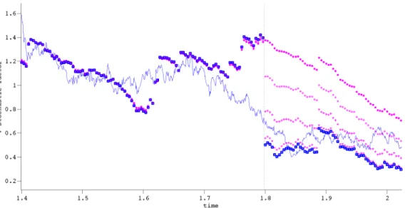
FDM is the operator stabilisation. In system theory, the concept of stability is in general referred to the sensitivity of the solution to a small perturbation of the system parameters, usually the initial conditions. In the application of nite dierence schemes for the solution of PDEs and in particular to evolutionary problems, the study of the stability of the operator approximation is concerned with the problem of suitably choosing the discretisation scheme for the time variable, in order to assure the stability of the solution approximation, seeTavella and Randall(2000),Duy(2006). In reality, it would be more appro-priate to dene this problem as how to preserve stability when moving to the time discretisation scheme, assuming the operator in the space dimension is initially stable. However, if we disregard the special role that is assigned to time, we might think of this problem for FDM as the problem of stabilising the time-space operator, altogether. In the particular implementation chosen in this paper, we avoid the last issue by taking the analytic solution of the space dimension discretised problem. As a consequence, we are left with the study of the stability of the space-discretised operator. In this section, we take into consideration the stability aspect of the matrix approximation of the original PIDE problem, and provide a criterion which is exploited as a tool for the analysis of this aspect of the likelihood approximation. The design of a stable system is crucial in the construction of the estimation procedure. We oer some guidelines in what follows, without the pretence of exhausting the argument but more to shed some light onto the stabilisation issue related to the implementation of the AML procedure employed in this work. The stabilisation of the operator approximation is in general a task to be pursued on a case-by-case basis. In general terms, there is not an overall solution to the problem of the stability of a FDM operator and its study is usually conned to the derivative operator approximation∂. Considering the solution (16),
we search for system matrices with negative real part eigenvalues, which would grant stable solutions. However, not every nite dierence scheme grants stable operators. SeeTavella and Randall(2000) as to how to construct nite dierence scheme of any order. In Fig. 1we show a perfectly legit rst order rst derivative nite dierence scheme which produces a totally unstable matrix. The gure exhibits the real part of the matrix eigenvalues of a simple example whereby the use of a given nite dierence scheme produces a problematic approximation of a rst order derivative operator. The matrix eigenvalues are all positive entailing that the exponentiation of the matrix will rapidly explode at low variations oft. The
situation becomes even more intricate in the case of mixed derivatives with multiple dimensions, where the options to design a nite dierence approximation of a given order become numerous. As a general rule, we exploit the following version of the Gerschgorin's disks theorem. Let [aij] =:A ∈ Cn×n be a
square matrix andci=Pj6=i|aij|, we have
Theorem 3.1 (Gerschgorin, 1931). The eigenvalues of the matrixA lie in the union of the disks {z∈C:|z−aii| ≤ci},1≤i≤n
Therefore, the general criterion in constructing a FDM scheme consists of plugging as many negative values as possible on the matrix operator diagonal and keeping the radius of the disks small, in order to obtain stable dierential operator approximations. In Fig. 2, we show the ordered real part of the eigenvalue of the matrix approximation of the operators ∂x, ∂2
xx and ∂xv2 , which have been used in the
empirical section. The careful choice of the dierentiation scheme allows for the complete stabilisation of the matrix operators.
To conclude this section, we recall that in the jump-diusion case with scalar point mark, we approxi-mate the jump operator with a trapezoidal rule that yields an approximation matrix, which is a triangular banded matrix. Usually, this matrix has a minor impact on the overall structure of the system operator. What can be said in general is that this matrix contains positive entries, therefore it will shift the centre of the Gerschgorin's disks to the right, determining a cause for the decrease of the stability. Another problem is related to the fact that although the individual operator blocks might be stable or negligibly destabilising, their sum does not necessarily retain the same spectral structure of the individual factors. Moreover, a few problematic eigenvalues might have been generated by numerical truncation that exhibit a positive real part which tend to shrink when increasing the thickness of the grid. For instance, in the following table5 we compare the percentage of the matrix trace which can be attributed to problematic
eigenvalues for several approximations of the full operatorAX+JX:
5The table exibits the value of the index in corresponding to a given grid dimension. The correspondent matrix
approx-imation of the PIDE operator is a square matrix whose side is as long as the grid volume expressed in terms of number of steps for each dimension. That corresponds to all the possible combinations of the coverage of the values allowed by the multi-dimensional grid. The index shows the percentage ratio of the sum of the absolute value of positive real part
grid dimension instability index
10×10 2.27% 20×20 0.16% 30×30 0.04% 50×50 0.00%
We observe that they tend to disappear when the system dimension increases, that is the grid becomes more dense.
In practice, it is important to remark that before using a PIDE solution for the design of the AML procedure, a preliminary study of the system state distribution function output must be run thoroughly and the system grid must be carefully chosen, in order to calibrate the algorithm. Having chosen a xed grid approach, it is important to make the multi-interval proportionate to the long-run variability of the system components and further rendering a suciently ne grid in order to obtain a well enough detailed distribution at low variability levels. The point of strength of this approach is that it is easily adaptable for any type of multivariate jump-diusion model, whereby the implemented codes require only few modications to change the system state equations. Moreover, it allows the parameter estimation time to be greatly reduced showcasing the benet of the sole need of one single matrix exponential at each likelihood cycle, leaving ample possibility for a targeted implementation of the numerical algorithm at the programming level. The procedure also oers the possibility of cutting o the numerical gradient loop, at the cost of a further matrix exponentiation, cfr. Van Loan(1978). We leave this latter step to subsequent implementation and testing.
4 Experimental Section
In this section, we provide empirical evidence in a simulated environment of the ecacy of the described procedures for the estimation of jump-diusion models. We deal with a stochastic volatility model with jumps whose diusive component may have a non-ane state function volatility, while the jump com-ponent is characterised by a state dependent stochastic intensity which can be non-linear as well. The approach is particularly appealing for the ltering of non-ane processes, where we cannot use, for exam-ple, the spectral ltering procedure as inBates(2006), and even so, in the ane case the jump-diusion ltering proposed in this paper is particularly convenient. In fact, for the implementation of the cited approach, the estimation of the latent state requires the combined use of numerical integration and dif-ferentiation of the characteristic function, constructed via the solution of the ODE system associated with the ane model, cfr. Due et al. (2000). On the contrary, the extended lter introduced in this paper and constructed directly in the time domain, produces estimates of the system state trajectories through the less complex recursion described by the Eqs. (8), (9) and (13), an implementation strategy that requires a lower number of approximation layers. Concerning the parameter estimation exercise, the PIDE approach used here is instrumental to the optimisation of the model parameters by which a sample path is most likely to have been generated, and the attention is more for the implications in the ltering context. We refer to articles such as Jensen and Poulsen (2002), Lindström (2007) for a comparative analysis of the AML adopted in this section.
With the Monte Carlo experiment, we check that the estimation of the system state and the model parameters are signicant, while focusing the analysis on several aspects of the system development and estimation that we have found to be relevant. Specically, we augment the system state of the stochas-tic volatility model with the integrated variance dynamics y1 and produce statistical evidence that it
brings signicant information into the system for the sake of the estimation of the latent state voolatility. Further, introducing a measurement error in the observation equation (19), we test the autocorrelation function of the output residuals to investigate the white noise hypothesis, nding that the strong auto-correlation and the presence of a unit root suggest to model they1's residual in a martingale form that
entails the augmentation of the state equation by the measurement error, as it was an auxiliary latent variable. Moreover, while experimenting several model specications as a jump-diusion inxwith a pure
diusivev factor, we have detected the presence of unexpected jumps in the projection of the variable v. In the latter situation, we provide evidence that this phenomenon, when present, may be corrected
with a pure jump measurement error, which is probably the most suitable form for the measurement error, when the lter is applied to jump-diusions. Further down the line, we investigate its nature by questioning the need of a measurement error. In fact, we provide evidence that in the majority of the extreme cases, the presence of a jump in the supposedly pure diusivev factor can be accommodated by
eigenvalues over the sum of the absolute value of the full set of eigenvalues. That number can be thought of as an index of instability of the system matrix: the lower the better.
dropping the variableE and by the likelihood estimation of the parameters. Finally, with another AML
exercise, we exhibit the parameter estimates and their likelihood derived standard error, highlighting the very low tracking error of thev estimates with respect to the simulated ones and whereby we also show
how to use the lter to derive an estimate of the jumps. The main statistics are presented in Tabs. 2and3. The simulations are produced with a simple Euler scheme at a very tight interval, plus the product of the jump size times a binomial random variable withpt= 1−exp [−λ(Xt)∆t].
4.1 System Design
In this section we characterise the form of the system used in the Monte Carlo experiments. We introduce the SDE describing the dynamics of the system and its observables. The baseline state equation is given by dx = θpqx(v) dW0 (18) dv = κ(ω−v) dt+σ√vρdW0+ p 1−ρ2dW 1 +JvdN1 du = θ2qx(v) dt dπx = −J0dN0 dπu = J02dN0
The dynamic system described by the Eqs. (18) represents the state of the reference multi-variate process we are employing for the Monte Carlo study. The observation equation is given by the linear form
y0 = x+πx (19)
y1 = u+πu+ε
The observations are represented by the two dimensional vectorY = (y0, y1). The processy0 is a
jump-diusion with quadratic variation given by the (Lebesgue)-stochastic integral R
dtθ2qx(v) + ¯J02λN0,
representing the prototype stochastic volatility model for the experimental exercise. As it can be no-ticed, the quadratic variation of y0 depends on the instantaneous variance of the pure diusion x and
the second order (innitesimal) moment of the Poisson random measure, symbolically described by the stochastic dierentialdπx. The parameterθis a scaling factor, whereas the diusion function is taken as qx=v2γ, with0< γ <1. This specication corresponds to a deterministic constant elasticity function6.
Given the dynamics ofv, basically the constant parameterγregulates the skewness of the unconditional
distribution of the unscaled diusion, determining an asymmetric response in the functionvγ, whenv tis
below or above the long run average of one. The caseγ= 1/2corresponds to an ane volatility function.
The state componentv is a scalar square-root process, which can be aected by jumps N1 that are not
synchronised with the jumpsN0 in y0 and that have independent size distributions. The inclusion of a
jump in volatility allows the system to resemble the behaviour of the double-jump model introduced by
Due et al. (2000). Other working hypotheses can be easily implemented. We allow for the presence of correlated diusive random drivers between the factorxand the stochastic volatility factorv, a fact
that in applied nancial econometrics is used to reproduce the so called leverage eect, cfr. for instance
Glosten et al. (1993). However, we notice that this feature might be reproduced by suitably modelling the jumps and the intensity function. The variablevis also input to the state dependent jump intensities λN0(v), which can be a linear or a square function ofv, allowing state dependency and non linearity also
in the stochastic jump-intensity process that have been handled by the jump-extended lter introduced in this paper. For the specic simulation experiment where the jump in varianceN1 is considered, its
jump intensity and that of N0 will be taken as linear in v with the scaling factor of λN1 given by a
xed proportion of the parameter λN0. As they are conceived, the stochastic intensities will produce
clustered jumps manifesting their concentration during volatility peaks. The simple non-linear stochastic intensity model with jump frequency described byλ0v2, will exacerbate the feature just described. The
jumps in volatility are assumed to have an ane intensity, with a coecient which is a xed fraction of
λ0. The jump size distribution of the Poisson point process component J0 is specied as exponential,
which is also the case forJ1, or extreme value distributions, depending on constant parameters. In the
latter case, the jump size distribution is given by the polynomially decaying extreme value distribution
P[J0≤z] = 1−(1 +z/α)−
η
, where we need to require nite order fourth moments in order to grant the well deniteness of the time-propagation equation. In the appendix (cfr. A.5) we calculate the moments
6In economics, the elasticity of the utility functionU(c)is dened as−cU00/U0. This corresponds to an elasticity of the
of the extreme value distribution function used in the experiments. We notice here another interesting aspect of the estimation approach presented in this paper, that is the ability of handling extreme value distributions (EVD) for the jump size, a characteristic that is prevented by the requirement of nite exponential moments in the jump extension of the indirect Hermite expansion approach of Aït-Sahalia
(2002) , cfr. Filipovi¢ et al. (2013) and Singer (2006). The coecient ω = (κ−λ0Jv¯)/κ, allows the
stochastic factorvto oscillate around one with unconditionally unitary mean. For that, in the estimation
exercise we will require the mean reversion speed to be higher than the jump drift, in order to obtain stationary variance. As it can be noticed, the jump processN0is not compensated, hencey0will have a
negative drift. Another key point in the design of the system state is the isolation of the diusion from the jump components, such that the lter state estimates will produce a direct estimate of the the jump process itself. However, this strategy is not directly implementable for the jump component in the v
factor, because it does not enter directly in any observable. As it will be seen in the AML exercise, the estimation of this feature is problematic.
The observable y1 plays a special role. As the state vector (x, v, πx) is completely unobservable
with a dimensionality which is higher than that of the observabley0, we would expect a high degree of
indeterminacy in estimating its projection ontoGt. However, for the case under analysis, we can resort
to stochastic calculus to obtain two new variables which increase the information content available by introducing a new observable. We plug into the observation equation the integrated variance of the processy0, which is partially observable. We will prove later that this innovation matters. The integrated
variance has been used in other applications in a realised volatility context, see for instance Bollerslev and Zhou(2002), which exploits its moment structure to improve the estimation of a stochastic volatility model. In this paper, the origination point is dierent. We construct the processy1=u+πuconsidering
the SDE which describes the observabley0=x+πx and derive the process dynamics forw=y02 dw = 2y0 c0dt+θ p qx(v) dW0 +θ2qx(v) dt+(y0−J0)2−y02 dN0 = 2y0dy0+θ2qx(v) dt+J02dN0 = 2y0dy0+ du+ dπu. Hence, lety1=w−2 R
y0dy0 to obtain the new observabley1. The augmented state vector for the
simu-lation exercise is thereforeX = (x, v, u, πx, πu). In deriving the reference state equation, we highlight the
separation of the main random sources into specic state variables, a design choice that allows for the dis-entangling of the jump variable from the diusion component. As a consequence, the lter Eqs. (18) and (19) will be able, in particular, to produce the projection of the latent variableπx, which accumulates the
jumps of the observabley0. We will use the latter lter output to estimate the jump times and sizes;
sim-ulation shows that the jumps can be estimated as the tail events of the rst dierence distribution of the cumulative jump state component, when the tail is cut at the expected unconditional frequency of jumps. The residuals after the distribution cut, can be seen as a projection error that is expected to be negligible. At this stage of the construction of the stochastic system to be used to experiment the non-linear lter complemented with the chosen AML procedure, we have not yet introduced any measurement er-ror process. We introduce the variable E = ε into the denition of y1, as in Eq. (19), postulating a
further stochastic factor in explaining the dynamics of the observations for the sequencey1(tn), n∈N.
However, some questions are crucial in the design of an ecient lter. In the following, we pay partic-ular attention to the form that εis most likely to exhibit and the implications that entails; further we
question the introduction of an additional unobserved process in the system, such asε. Concerning its
form, the classical hypothesis in ltering is that the measurement error is a white noise εt. However,
when introduced into the system, the residuals that it gathers contradicts this simple hypothesis. We followDempster and Tang (2011) in modelling directly the measurement error within the system state and extend this concept further by allowing the measurement error to be aected by jumps. When it is not taken as a simple white noise, the general form of the error is a scalar version of Eq. (14), where its diusion or pure jump form will be used separately. The empirical evidence shows that in the presence of jumps, a pure diusion system state component, like v in the experiments carried out in this paper,
might in extreme cases exhibit jumps which have not been modelled and that can be accommodated by the introduction of a jump latent measurement error variable. However, the introduction of an auxiliary variable employed as a measurement error for the observation equation might be redundant. In fact, in a simulation exercise presented below, we gather evidence showing that the latter feature is likely to be due to unoptimised parameters. It is further to be noticed that dropping the variableεcan be justied
by the presence of a non-zero residual in the cumulative jump projections, once that the jump estimates have been removed. This characteristic signals that in the presence of jumps some background noise in
the observation equation might be absorbed by the jump projection.
For the illustration of the AML estimation procedure, the system (18) is re-elaborated in order to construct a simplied version of the likelihood function. We deal with the stochastic volatility system in Eq. (18) whereby the integrated variance component has been dropped. In the latter case, the observation error is irrelevant for the parameter estimation exercise. We produce estimates for the two dimensional system(x0, v). In constructing the likelihood iteration, we apply the approach depicted in the estimation
dening Section 3. We remark that the system state and the observables are, respectively,X= (∆x0, v),
Y = ∆y0. Hence, we get the following iterations for the target likelihood:
P(Xt+1|Yt) =at
Z
dvtP(∆x0,t+1, vt+1|0, vt)P(∆y0,t, vt|∆y0,t−1) (20)
The log-likelihood function for the observables is then
LN = N1Σilogati
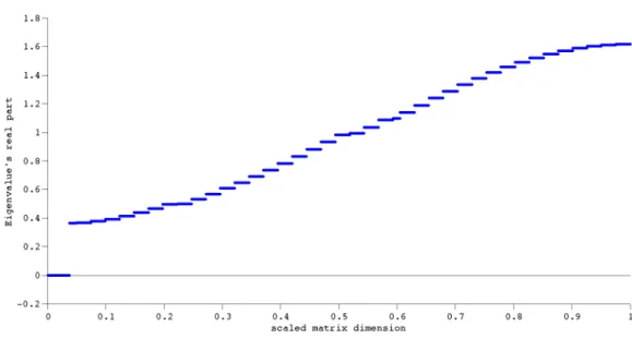
Ultimately, the AML module constructed in Section 3 provides a moderately time consuming algorithm for the estimation of continuous time parametric models. The integrals involved in the likelihood iteration are discretised to obtain simple matrix multiplications on the dened grid. The full vector of the output parameters is the set(θ, κ, σ, ρ, γ, λ0, α0, η), which represents, respectively, the diusion scaling factor for
the observed variable x, the speed of mean reversion constant for the stochastic factor v, its volatility
coecient, the correlation factor of the diusion stochastic factors of x and v, the diusion exponent
factor and the diusion scaling factor. The remaining factors have dierent use according to the model they are used for; theαparameter is a scaling parameter for either the exponential or the extreme value
jump size distribution, whereasηis employed either as the exponent factor for the EVD or as the scaling
factor for the exponential distribution for the jump in thevfactor. Whenever unused, certain parameters
are dropped.
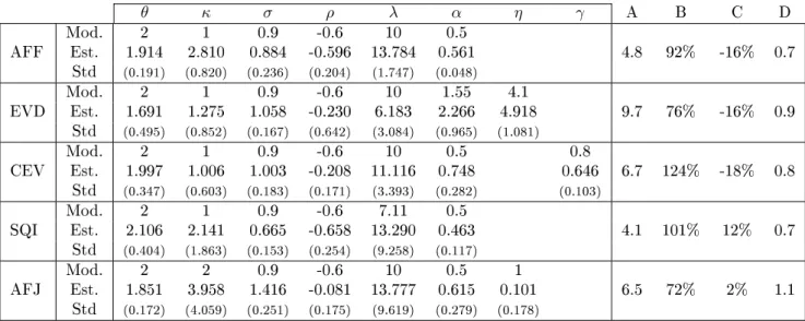
4.2 Diagnostic check of the system state specication
In the rst set of tests, we include the integrated variance into the system and provide statistical evidence of its statistical signicance. We postulate a martingale form for the measurement error which is tested successively in a second set of diagnostic checks, where we want to establish the most likely form of the measurement error. Table2 provides the summary results of the test statistics constructed in this rst part of the empirical section; Table1contains a legenda of the acronyms used in the latter table. In most cases, the only variables that are left free are the measurement error parameters, while the system state parameters are set at the simulation values. In the case of the testing for the exclusion of measurement error, the model parameters have been estimated with AML. We include several ane models, that also include jumps, which are kept at quite a high frequency, when testing for jumps in the ltered path of a pure diusionv. We use the quasi-analytical approximation for ltering non-ane model specications
as the CEV and the squared jump intensity. The drift induced by the jump component is the same for the exponential and EVD jumps size, whereas in the case of the squared jump intensity it is slightly smaller, to compensate for the higher variability generated by the squaring of thevfactor. The expected
jump size is the same for all the models. The integrated variance
Bollerslev and Zhou(2002) use several sample moments of the integrated variance of equity prices, to estimate parametric stochastic volatility models with the method of moments. The background idea is to extend the information available from observed data to improve the performance of the estimation function. Their main focus, however, is on realised volatility with high frequency data. In this paper, we employ the same idea of extending the observable set, but from a dierent perspective. We manipulate the state equation to obtain the dynamics of the squared variation, which, up to the integral approx-imation, is observable. The integrated variance components are then included in the augmented state vector, as in Eq. (18), while a new observable,y1, is obtained. The question we answer in this section is
whether this extension is signicant in terms of the estimation ability of the latent state ofv. However, in
some cases the inclusion of the variabley1could even be necessary before being signicant. For instance,
the lter considered in the estimation exercise with ρ = 0 and lacking the variable y1, for any initial
condition, would be able to produce only a curve decaying to the long run mean, because the absence of correlation completely disconnects the projection of the latent state from the observablex. The latter
feature is related to the intrinsic martingale structure by whichxhas been modelled.
We introduce the integrated variance of the processxin order to augment the information used by the
lter to produce the latent state estimation. We prove here that the inclusion of the integrated variance within the system steers a signicantly informative data ow to the ltering device. We test the latent statevestimation ability of the lter with or without the integrated variancey1. In case of a system with
the latter variable, we include the measurement error ε which we assume to be a martingale diusion.
The model parameters are set to their simulation values, whereas the error parameter is optimised by minimising the mean squared error (MSE) of the y1 against the ltered one. The estimation ability of
the lters is measured with the sample MSE, E(v−v¯)2, of the ltered ¯v path. We apply the t-test
and the F-test on a large sample of model paths, yielding a set of sample MSE's. The test results are presented in Tab. 2, labelled test T0. The null hypotheses are based on the assumptions that the plain
lter without the integrated variance is yielding a MSE which is on average lower and less volatile than those produced by the augmented state lter. The hypotheses correspond to the irrelevance of the lter with an extended observation equation. We consider the case of a pure diusion x, whereby it should
be easier to estimate the variance path as the variance of the observable which is generated totally by a single risk factor. The models encompass ane and non-ane specication, with a constant elasticity of variance specication, with the parameterγ ranging from0.2 to 0.9. Nevertheless, the null hypotheses
are strongly rejected in all the cases under analysis. It is interesting to notice that in the ane case withρ= 0 the reduced state model produces not only a signicantly higher MSE on average, but it also
generates a huge variability of this performance measure. The same happens in the case of the highly sensitive response of thex's diusion to the vfactor.
A martingale measurement error
In the previous section, we have assumed that the augmented observation Eq. (19) contains a measure-ment error ε which is a martingale diusion. In this section, we include the y1 variable and test that
the latter assumption concerning the measurement error is the most likely. As a consequence, with the martingale assumption, the system state is augmented with theεdynamics specication.
With the test labelled T1we rst verify whether assuming a white noise structure for the measurement
error is preferable to a martingale equation. With a large sample, that is2,000 sample paths generated
for a simple ane pure diusion with quite a high diusion coecient for the latent factor v and high
negative correlationρ, we perform a dual tail t-test and F-test for the null that, respectively, the ex-post
MSE average and variance of the estimated sample pathv¯ against the realised trajectories are dierent
within the two samples. We found that these hypotheses are strongly rejected, supporting the conjecture that using a white noise or a martingale form forεare equivalent. However, this approach is not optimal.
In fact, with the sequence of tests labelled T2 and T3, we check for the autocorrelation presence in the
residuals and even for the presence of a unit root in lag polynomial of, respectively, the sample residuals of the white noise and the martingale measurement error form. Again, we choose a simple model structure, that is that of a pure diusion ane model. In this case already, the results are clear. We randomly select from a 2,000 sample path for several model parameter specications, two sample paths upon which we perform a Phillip-Perron test for the presence of unit root and an augmented Dickey-Fuller test for the presence of autocorrelation. The time series which are investigated are the sample measurement error y1−y¯1 output of the ltering algorithm. In the case of the martingale error with the test T3,
the autocorrelation of the residuals are tested after the application of the rst dierence operator, as for the conrmation of the unit root presence. The unit root presence is strongly rejected in the white noise case (test T1), but the presence of autocorrelated residuals is always conrmed. In the case of
the martingale specication of the measurement equation, as in the case of the group of tests T3, we
nd very general conrmation of the unit root presence, which is removed by the application of the rst dierence operator, which is to say that the Dickey-Fuller test generally fails to reject the absence of autocorrelation. This battery of tests on random samples taken from model specication characterised by high and low variance of the latent factorv along with presence and absence of correlated random
drivers provides strong evidence for the adoption of the martingale hypothesis, via the inclusion of the measurement equation within the system state. It is interesting to notice the results of the tests T2-A and
T3-A, whereby the unit root presence is in the rst case rejected and in the second case conrmed. Those
results are produced by two dierent measurement error specications suggesting that the autocorrelated residuals might be self-induced by the smoothing feature of the ltering device. The optimal strategy to deal with this feature is adopting a martingale form which delivers coherent results for both the experiments.