Relax, descend and certify : optimization techniques for typically tractable data problems

Copyright by

Maria Soledad Villar Lozano 2017

The Dissertation Committee for Maria Soledad Villar Lozano certifies that this is the approved version of the following dissertation:

Relax, descend, and certify: optimization techniques for

typically tractable data problems

Committee:

Rachel Ward, Supervisor Afonso S. Bandeira Andrew J. Blumberg Arie Israel

Relax, descend, and certify: optimization techniques for

typically tractable data problems

by

Maria Soledad Villar Lozano, B.S., B.Eng., M.S.

DISSERTATION

Presented to the Faculty of the Graduate School of The University of Texas at Austin

in Partial Fulfillment of the Requirements

for the Degree of

DOCTOR OF PHILOSOPHY

THE UNIVERSITY OF TEXAS AT AUSTIN May 2017

Acknowledgments

I have the deepest feelings of gratitude and admiration to my advi-sor, Rachel Ward, who has taught me, encouraged me, shared great math ideas, and given me amazing opportunities throughout my PhD.

I am also very grateful to have such talented mentors like Dustin Mixon and Afonso Bandeira. I truly appreciate their support, our very en-lightening math discussions, and their friendship.

I am very fortunate to have amazing collaborators. This thesis is in fact based on different projects with multiple coauthors: Pranjal Awasthi, Afonso Bandeira, Andrew Blumberg, Timothy Carson, Moses Charikar, Rav-ishankar Krishnaswamy, Takayuki Iguchi, Dustin Mixon, Jesse Peterson, and of course Rachel Ward. I am thankful I had the opportunity to work with every single one of them.

I thank my thesis’ committee members for the feedback provided. In particular I am grateful to Arie Israel for his sharp comments that greatly improved this manuscript.

I appreciate the help and support from faculty and staff from Uni-verisity of Texas at Austin, in particular Andrew Blumberg, Bubacarr Bah, Dan Knopf, Sandra Cattlet, Thomas Chen and Elisa Bass.

Tornaría, for his central role in my mathematical education and in me com-ing to Austin.

The Uruguay Math Olympiads has played an important part inspir-ing my mathematical curiosity from a very young age. I want to thank Ariel Affonso and everyone that made this unusual career path even possible for me, and everyone who through the Uruguay Math Olympiads is inspiring young kids to love math as I do.

I thank my friends in Uruguay and Austin for their invaluable friend-ship, and in particular Tim for making me happier every day.

Lastly but most importantly I want to acknowledge my family, spe-cially my parents Pilar and José, and my sisters Andrea and Florencia, for being the most important invariant in my life.

Relax, descend, and certify: optimization techniques for

typically tractable data problems

Publication No.

Maria Soledad Villar Lozano, Ph.D. The University of Texas at Austin, 2017

Supervisor: Rachel Ward

In this thesis we explore different mathematical techniques for ex-tracting information from data. In particular we focus in machine learning problems such as clustering and data cloud alignment. Both problems are intractable in the "worst case", but we show that convex relaxations can efficiently find the exact or almost exact solution for classes of "typical" in-stances. We study different roles that optimization techniques can play in understanding and processing data. These include efficient algorithms with mathematical guarantees, a posteriori methods for quality evaluation of so-lutions, and algorithmic relaxation of mathematical models. We develop probabilistic and data-driven techniques to model data and evaluate per-formance of algorithms for data problems.

Table of Contents

Acknowledgments v Abstract vii List of Figures xi Chapter 1. Introduction 1 1.1 Clustering . . . 3 1.1.1 A remark on finding the number of clusters . . . 6 1.2 Gromov-Hausdorff distance and point cloud matching . . . 7 1.3 Relax-and-round versus exact recovery . . . 9 1.4 Main contributions . . . 10 1.4.1 Relaxations of thek-means problem . . . 10 1.4.2 Exact recovery of clustering solutions using

con-vex relaxations . . . 13 1.4.3 Fast certification ofk-means optimality . . . 19 1.4.4 Approximation guarantees . . . 21 1.4.5 A polynomial-time relaxation for the Gromov-Hausdorff distance . . . 24

Chapter 2. Background 27

2.1 Optimization . . . 27 2.1.1 Cone programming . . . 29

2.1.1.1 Complementary slackness and dual cer-tificates . . . 30 2.1.2 Manifold optimization . . . 31

Chapter 3. Manifold optimization techniques fork-means clustering 34

3.1 Thek-means manifold. . . 34

3.2 Gradient of the objective function . . . 36

3.3 Projection of a vector ontoTYM. . . 37

3.4 Homogenous structure ofM . . . 38

3.5 Splitting the tangent space toM . . . 40

3.6 A retraction map . . . 41

3.7 Numerical algorithm . . . 42

3.8 Numerical simulations . . . 42

3.9 Discussion . . . 43

Chapter 4. Finding the exact solution: tightness in convex optimiza-tion 46 4.1 A semidefinite program relaxation fork-means . . . 46

4.1.1 Dual certificate from separation condition . . . 52

4.1.2 Dual certificate from spectral condition . . . 58

4.1.3 Integrality of the relaxation under the stochastic ball model . . . 62

4.1.3.1 Proof of Corollary 4.1.8 . . . 63

4.1.3.2 Proof Theorem 4.1.9 . . . 65

4.2 Integrality for thek-medians LP relaxation . . . 75

4.2.1 Proof of Theorem 4.2.2 . . . 82

4.2.2 Proof of Theorem 4.2.3 . . . 83

4.3 An integrality gap for thek-means LP relaxation . . . 89

Chapter 5. Efficiently certifying exact solutions 94 5.1 A fast test fork-means optimality . . . 99

5.1.1 Leading eigenvector hypothesis test . . . 99 5.1.2 Testing optimality with the power iteration detector 105

Chapter 6. Approximation guarantees for relax and round algorithms110

6.1 The relax-and-round algorithm . . . 111

6.2 Performance guarantee for thek-means SDP . . . 112

6.3 Proof of Theorem 6.2.2 . . . 117

6.4 Denoising . . . 126

6.5 Rounding . . . 130

6.5.1 Numerical example: Clustering the MNIST dataset 132 Chapter 7. Polynomial-time lower bound of NP-hard functions 136 7.1 Semidefinite programming relaxations of Gromov-Wasserstein and Gromov-Hausdorff distances . . . 139

7.2 Topological properties of the relaxed distances . . . 145

7.2.1 Pseudometrics . . . 145

7.2.2 Monotonicity and continuity properties . . . 151

7.2.3 Extension of the distance to compact infinite sets . . 152

7.2.4 Comparison with the Gromov-Hausdorff distance . 153 7.2.5 Topologies induced by relaxed distances . . . 154

7.2.6 Local topological properties . . . 156

7.3 GHMatch: a rank-1 augmented Lagrangian approach to-wards the registration problem . . . 158

7.4 Numerical performance . . . 161

7.4.1 Classification using the distance ˜d_GH . . . 161

7.4.2 Performance of GHMatch . . . 163

Bibliography 167

List of Figures

1.1 Illustration ofk-medians andk-means . . . 4

1.2 Peng and Wei’s semidefinite programming relaxation of (k-means) . 14 1.3 Linear programming relaxation of (k-means) . . . 14

1.4 Linear programming relaxation of (k-medians) . . . 14

1.5 Stochastic ball model. . . 15

1.6 Failure of Lloyd’s algorithm. . . 19

1.7 Illustration of the relax and roundk-means clustering procedure . . 23

3.1 Illustration ofYYT for iterations of Algorithm 1 with successive val-ues ofλ. . . 43

4.1 Illustration for proof of Lemma 4.2.4.. . . 86

5.1 Complementary slackness and probably certifiably correct algorithms 97 6.1 Clustering MNIST withk-means SDP. . . 135

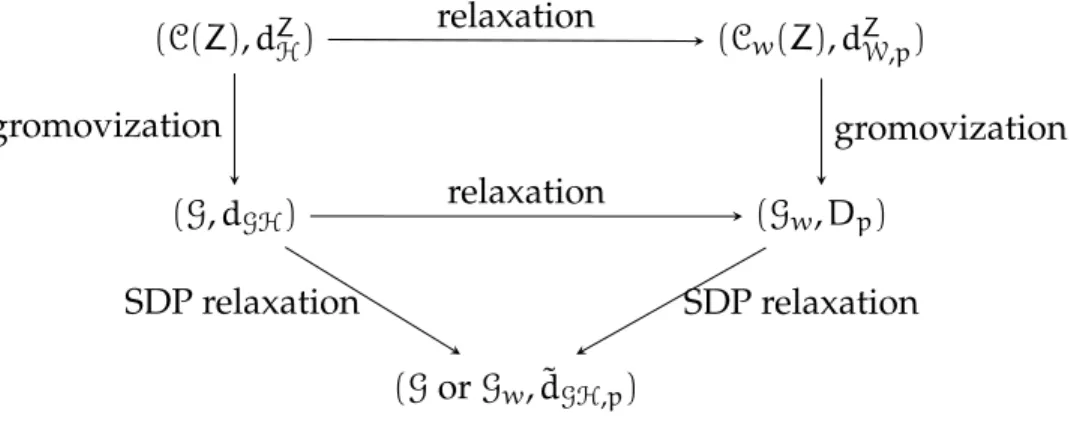
7.1 Diagram relating the different structures and distances . . . 144

7.2 Two non-isometric metric spaces that have relaxed distance 0. . . . 147

7.3 Visual comparison betweend_GHand ˜d_GH,1on a real data set. . . . 162

7.4 Convergence of GHMatch . . . 164

Chapter 1

Introduction

The problem of extracting knowledge from data is very relevant these days. The classical statistical approach for this kind of problem consists in the following steps (i) acquiring and processing data, (ii) formulating a statistical model depending on a few parameters, (iii) formulating a likeli-hood function of the parameters given the data, (iv) solving the optimiza-tion problem (finding the best parameters that maximize the likelihood for the given data).

The machine learning approach takes many of its techniques and ideas from statistics, but it formulates the problems in a slightly different way. For instance, supervised machine learning deals with large amounts of labeled data{(di,li)}n_i=1. Heredi∈Dcorresponds to data (for example an image), andli∈Lrepresents its label (for example ’dog’). Supervised ma-chine learning typically has a training step, with the purpose of inferring thebestfunctionf:D→Lthat adjusts to known information(di,f(d_i) =l_i). The function f is used to predict labels for new data. In a different man-ner, unsupervised machine learning finds hidden structures or patterns in unlabeled data, like clusters or manifolds.

Regardless of the approach to data modeling and processing, all these problems, at the end, amount to solving an optimization problem that can be expressed in the form

minimize fD(x) (1.1)

subject to x∈S.

whereD∈Drepresents the data of our problem in the universe of all pos-sible data D, and x represents a potential answer to the question we are asking about the data. The set of all possible answers isSwhich can be of many different shapes.

Optimization problems arising from data can be intractable in many cases. However, the computational complexity of a problem measures the amount of time or space that it takes to solve its hardest instance. For the problems we study in this thesis (and many other problems existing in the literature) it turns out that even NP-hard problems can be solved in polynomial-time for a large number of instancesD∈D. Compressed sens-ing is a famous example of this phenomenon [21].

In this thesis we focus on two data problems: clustering and point cloud matching. We study different approaches to their underlying opti-mization problem that allow us to:

(i) Find the exact solution of (1.1) for a non-trivial subset ofD.

(ii) Find an approximate solution of (1.1) for a larger subset of D, with explicit approximation bounds.

(iii) Leverage fast heuristic algorithms and mathematical proofs to develop quasi-linear time algorithms (in D) that provide the exact solution of (1.1) for a non-trivial subset ofD.

(iv) Substitute NP-hard functions by tractable proxies that preserve many interesting properties of the original functions.

This description may seem pretty abstract for now. A more concrete explanation is provided in Section 1.4, where we summarize the ideas for the specific problems. However, these techniques may be applied to seem-ingly any data-related problem.

1.1

Clustering

Clustering is a central problem in unsupervised machine learning. It consists of partitioning a given setP, a finite set of points of a metric space (X,d), into k subsets such that some dissimilarity function is minimized. The dissimilarity function is in general chosen with an application in mind. Due to the nature of most machine learning problems, identifying similar data is a main learning step and therefore many complex algorithms rely on clustering subroutines.

The clustering objective known ask-means is one of the most com-mon for data in Euclidean space, andk-medians is widely used in general metric spaces (like tree spaces). Figure 1.1 depicts both problems.

Figure 1.1:Illustration ofk-medians andk-means

Thek-medians objective (left) minimizes the sum of distances from points to their representative data points. Thek-means objective (right) minimizes the average of the squared euclidean distances of all points within a cluster.

the distance is the Euclidean distance d(xi,x_j) =kx_i−x_jk. The goal is to partition the finite set P={x1,. . .,xN}ink clusters such that the sum of the squared euclidean distances to the average point of each cluster (not necessarily a point in P) is minimized. Let A1,A2,. . .,Ak denote a partitioning of the the indices[N] ={1,. . .,N}intoksubsets; if

ct=_|A1_t|

P

j∈Atxjdenotes the centroid of the clustert, then thek-means problem reads minimize A1∪···∪Ak=[N] k X t=1 X i∈At kx_i−ctk2

By expanding the square one obtains the identity P_i∈Atkxi−ctk2= 1 2 1 |At| P i,j∈Atkxi−xjk

prob-lem as the following optimization probprob-lem: minimize A1∪···∪Ak=[N] 1 2 k X t=1 1 |At| X i,j∈At kxi−xjk2. (k-means)

k-medians The k-medians (also known as k-medoids) objective is defined for general metric spaces, where the notion of centroid may not exist. In this setting, clusters are specified bycenters: krepresentative points

from within the set P denoted byc1,c2,. . .,ck. The corresponding par-titioning is obtained by assigning each point to its closest center. The cost incurred by a point is the distance to its assigned center, and the goal is to findkcenter points that minimize the sum of the costs of the points inP: minimize {c1,c2,...,ck}⊂P n X i=1 min t=1,...,kd(xi,ct) (k-medians) Both problems can be expressed as an optimization problem of the form (1.1) whereD=P and S is a discrete set in correspondence with all possible partitions of the points ink clusters. Unfortunately, the combina-toric nature of the set of all possible partitions result in both problems being NP-hard [6, 36]. However, being NP-hard is a statement about the hardest instance of the problem; and there is a line of work that claims that cluster-ing is not hard when data is naturally clustered [12].

In fact, the geometric nature of thek-means problem allows a sim-ple and widely used alternating minimization algorithm known as Lloyd’s algorithm [43]. Lloyd’s algorithm consists of the following steps:

1. select random data points as centers, 2. assign each point to the closest center, 3. recompute centers,

where steps 2 and 3 are repeated until convergence. Lloyd’s algorithm is fast but it often converges to a suboptimal clustering, a local minimizer of (k-means). Not only that, but the output of the algorithm provides no information of how far from optimal it may be.

1.1.1 A remark on finding the number of clusters

Both thek-means andk-medians problem formulations assume that the number of clusterskis a known parameter. Sometimeskis given by the problem, for example in the hand-written digits data set that we study in Section 6.5.1, the number of clusters is 10. However, in many problems the number of clusters is not known a priori and should be estimated.

There exists a few techniques that allow us to find the number of clusters. One of the first methods to estimate the number of clusters is the el-bow method, that can be traced back to [60]. Informally speaking, the method consists of computing thek-means value for different values ofkand essen-tially choosingk?to be such that one does not gain too much when setting the number of clusters k=k?+1 and does not lose too much when with

k=k?−1.

Many methods have been developed since then. For example [69] presents a semidefinite program for clustering that chooses the number of

clusters, and [42] presents a spectral method to find the number of clusters.

1.2

Gromov-Hausdorff distance and point cloud matching

In order to study the convergence of sequences of metric spaces, Gromov introduced what is now called the Gromov-Hausdorff metric [30]. Roughly speaking, this metric generalizes the classic Hausdorff distance be-tween a pair of subsets of an ambient metric space, to a distance bebe-tween a pair of arbitrary metric spaces. This is done by embedding these metric spaces into a third space and taking an infimum over all such embeddings. The Gromov-Hausdorff metric has been of theoretical importance in geo-metric group theory and is at the heart of the subject of “geo-metric geometry”. More recently, the Gromov-Hausdorff distance has been proposed as a basic method for comparing point clouds[48]. A point cloud is simply a finite metric space (often presented as a subset ofRm); this is a fundamen-tal and ubiquitous representation of data. Geometric examples, where the point cloud represents samples from some smooth geometric object, arise from various kinds of shape acquisition devices. Examples with less ob-vious intrinsic geometric structure are frequently generated by biological data (e.g., collections of gene expression vectors). Given two point clouds, a natural question is to determine if they are related by some isometric trans-formation; if not, one might wish to know a quantitative measure of their difference.

Another version of this sort of problem is known as the point reg-istration problem (also sometimes referred to as point matching and net-work alignment). Point registration consists in finding a correspondence between point sets or graphs such that a certain cost function is minimized. It appears in computer vision problems like shape matching [25], computa-tional biology [22], and general pattern recognition problems. In some ap-plications, registering or aligning is particularly challenging since there is no explicit correspondence between the sets, often because deformation has occurred or they have different numbers of points. In such cases it is natural to consider a metric on point clouds that is defined in terms of correspon-dences between point clouds together; the Gromov-Hausdorff distance can be described in terms of a minimax expression over correspondences be-tween the metric spaces, and so is potentially suitable for this purpose.

Unfortunately, exact computation of the Gromov-Hausdorff distance is essentially intractable; it involves the solution of an NP-hard optimization problem. As a consequence, it is natural to consider relaxations. In [47], Mé-moli studied a relaxation referred to as the Gromov-Wasserstein distance — this distance is closely related to distances motivated by optimal trans-port problems [44, 59], to a “distance distribution” metric defined by Gro-mov, and also to the cut distance of graphons. Unfortunately, computing the Gromov-Wasserstein distance still requires solving a non-convex opti-mization problem which does not appear to have attractive performance characteristics in practice.

1.3

Relax-and-round versus exact recovery

A widespread idea to tackle these combinatoric optimization prob-lems is known as therelax and round paradigm. It consists in augmenting the discrete domain Sto a larger set ¯S where one can use optimization al-gorithms; solve the optimization problem in the larger set, obtaining ¯x∈S¯; and then round the solution of the relaxed problem into a feasible point of the original problem ¯x7→x?∈S.

If the functionf_D is convex, relaxing the optimization problem into a convex set ¯S results in a problem with a unique local minimizer, where interior point methods [51] are guaranteed to converge to global optima of the relaxed problem. If we provide an explicit bound for the differencekx¯−

x?kand a Lipschitz constant forfD, we obtain an approximation algorithm for (1.1) with explicit error bounds [63].

Sometimes we may also want to relax S to a non-convex set, for instance, a smooth manifold, where algorithms can be implemented very efficiently [14] but a priori are only guaranteed to converge to local op-tima (though under some hypothesis manifold optimization algorithms had been proven to converge to global optimizers [15]).

If the solution ¯xof relaxed optimization problem in ¯Shappens to be feasible for the original problem (1.1) (i.e.: ¯x ∈S), then ¯x is also optimal for (1.1). In such case we say the relaxation istightor that the relaxation has anintegralsolution.

1.4

Main contributions

1.4.1 Relaxations of thek-means problem

As mentioned before, one can rewrite thek-means problem as minimize 1 2Tr(DX) (1.2) subject to X:= k X t=1 1 |At| 1At1 > At,

whereDis ann×nmatrix such thatDij=kxi−xjk2, andXis a projection matrix into the span of the indicator vectors of each cluster (i.e.: (1At)i=1 ifxi∈Atand 0 otherwise).

An equivalent formulation fork-means is the following optimization in the set of rankkmatrices:

minimize 1

2Tr(DYY

>_{) (1.3)}

subject to Y∈Rn×k, YY>1=1,

Y>Y=Ik, Y_>0.

Here the constraintY>Y=Ik means thatYhas orthonormal columns. Using thatY_>0entry wise, we obtain thatYij6=0implies thatYik=0for allk6=j, so Y has exactly one nonnegative entry per row. The constraint YY>1=

1 implies that the vector 1∈Rn _{belongs to the span of the columns of Y.} Therefore if Y_ij 6=0andY_lj=6 0thenY_ij=Ylj. This shows that ifY is feasible for (1.3) thenX=YY> is feasible for (1.2).

Optimization problems (1.2) and (1.3) are equivalent tok-means, which is an NP-hard problem [6]. A typical way to tackle such hard problems is to

relax the discrete feasible set to a larger set, then use analytic tools to solve the larger problem, and finally round a solution of the larger problem into a feasible solution for the original problem.

For instance, thespectral clusteringtechnique is based on the follow-ing relaxation of (1.3):

minimize 1

2Tr(DYY

>_{) (1.4)}

subject to Y∈Rn×k, Y>Y=Ik.

Note that the solution of (1.4) is a matrix with columns consisting of the top

keigenvectors ofD.

In general, spectral clustering algorithms replace the matrixDby a matrix−K, whereKcorresponds to the Gram matrix of the points mapped to a higher dimensional space (i.e.: Kij =hφ(xi),φ(xj)i for φ :Rn →RN.) One particularly common implementation uses the Gaussian kernel: Kij = exp(−kxi−xjk2/σ2).

Another relaxation ofk-means, that we study in depth in this thesis, is Peng and Wei’sk-means SDP [56], which solves

minimize 1

2Tr(DX) (1.5)

subject to TrX=k, X1=1, X_>0, X0,

whereX0means thatXis symmetric and positive semidefinite. Note that the results from [23] indicate that the constraintX_>0is strictly weaker than the constraintY_>0.

The first relaxation we will focus on is amanifold optimization re-laxation ofk-means in Chapter 3. First note thatk-means can be seen as an optimization problem in a discrete set (the constraint set of (1.3)), but if we remove the non-negative constraintY _>0 we obtain a compact manifold. We consider the relaxation of (1.3) where we relax the non-negative con-straintY_>0to a penalization in the objective, and restrict the minimization toY∈MwhereMis a smooth submanifold ofRn×k:

minimize Tr(DYY>) +λkY−k2F (1.6) subject to Y∈M.

HereY− indicates the negative entries of Y, λ is a non-negative parameter that penalizesYwith negative entries, andMis the submanifold

M={Y∈Rn×k: Y>Y=Ik, YY>1=1}. (1.7) By removingY_>0from the constraint set, our discrete feasible set becomes a smooth manifold without boundary, so we can use manifold optimization algorithms to solve the problem.

Also note that adding the constraint YY>1=1 to spectral clustering is simple and doesn’t change its spectral nature (in particular, if λ=0 the solution can be computed from the topk−1eigenvectors of the projection ofDonto{1}⊥⊂Rn_{). What makes this optimization significantly different} from spectral clustering is the termλkY−k2_Fin the objective.

In Chapter 3 we explain how to implement an efficient manifold op-timization algorithm to approach problem (1.6) and we provide numerical

experiments that suggest that, in some settings, the algorithm converges to the optimal solution of (k-means). Unfortunately we do not have theoreti-cal guarantees for this algorithm yet (the objective of (1.6) is not convex and the algorithm may converge to local minima). However, we will be able to combine this efficient algorithm with the proofs from Chapter 4 to provide an efficient algorithm with a certificate of optimality in Chapter 5.

1.4.2 Exact recovery of clustering solutions using convex relaxations We consider three different convex relaxations of thek-medians and

k-means objectives, described in Figures 1.2, 1.3, and 1.4.

(i) A semidefinite programming (SDP) relaxation ofk-means introduced by Peng and Wei [56],

(ii) a linear programming (LP) relaxation ofk-means,

(iii) and a standard linear programming (LP) relaxation ofk-medians, See Section 2.1.1 for a brief background in linear and semidefinite programs.

We provide deterministic conditions that if satisfied by the point set

P, imply that the corresponding convex optimization program is tight (and therefore it recovers the exact solution of problems (k-medians) or (k-means)).

The deterministic conditions we find do not provide geometric intu-ition a priori. Therefore, in order to evaluate their expressivity, we consider a random point model of naturally clustered data introduce by Nellore and Ward [50] known as the stochastic ball model depicted in Figure 1.5. The

minimize X∈RN×N

1

2trace(DX) (k-means sdp)

subject to X1=1, trace(X) =k, X_>0, X0.

Figure 1.2:Peng and Wei’s semidefinite programming relaxation of (k-means) The symmetric matrix D is defined as D_ij :=kx_i−x_jk2 _forx

i,xj∈P, and X0 means that Xis symmetric and positive semidefinite. IfA₁,. . . A_k is a cluster, the corresponding projection matrix XisPk_t=1|A1

t|1At1

>

At where the indicator vector

(1At)iis 1 if xi∈At and 0 otherwise. Note that relaxation (k-means sdp) relaxes

the set of all cluster projection matrices into a subset of the positive semidefinite matrices. minimize X∈RN×N 1 2trace(DX) (k-means lp) subject to X1=1, trace(X) =k, X=X>, Xii>Xij∀i,j∈[n], Xij>0. Figure 1.3:Linear programming relaxation of (k-means)

This linear programming relaxation replaces the semidefinite constraint from (k-means sdp) with looser linear constraints. In general, linear programs are nu-merically more efficient and simpler to analyze than semidefinite programs. How-ever we prove the quality of the solution of (k-means lp) is inferior to the one of (k-means sdp). minimize z∈RN×N_,y∈RN n X i=1 n X j=1 d(xi,xj)zij (k-medians lp) subject to n X i=1 zij=1∀j∈[n], zij6yi∀i,j∈[n], n X i=1 yi=k, zij,yi∈[0,1].

Figure 1.4: Linear programming relaxation of (k-medians)

The relaxation (k-medians lp) consists of replacing the discrete set{0,1}by the in-terval[0,1]. In the original optimization problem (k-medians) the variabley_i indi-cates whether the pointx_iis a center or not, whilez_ijis 1 if the pointx_jis assigned toxias center, and 0 otherwise. The solution for the integer programming problem (where{z_ij,y_i}∈{0,1}) corresponds to the adjacency matrix for a graph consisting of disjoint star-shaped graphs like the one shown in Figure 1.1.

premise behind evaluating algorithms in this model is that a good algo-rithm should recover the right clusters when the solution isobvious.

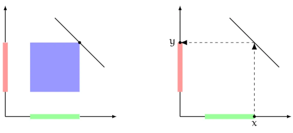
Figure 1.5:Stochastic ball model.

Example of an instance of the stochastic ball model inR2. HereDis the uniform distribution in the unit ball,k=3,n=15, and∆=2.2.

Definition 1.4.1((D,γ,n)-stochastic ball model). Let{γa}k_a=1be ball centers inRm. For eacha, draw i.i.d. vectors{ra,i}n_i=1from some rotation-invariant distributionDwhose support is the unit ball. The points from clusteraare then taken to bexa,i:=ra,i+γa. We denote∆:=mina6=bkγa−γbk2.

Note that when∆ < 2the the clusters overlap and the "cluster solu-tion" is no longer well-defined. We now present informal statements of our main results; see specific sections for more details.

Theorem 1.4.1. Under(D,γ,n)-stochastic ball model and with high probability, Peng and Wei’s SDP relaxation ofk-means (k-means sdp) recovers the clusters up to separation∆ >min{2p2(1+1/m), 2+k2/m}.

Theorem 1.4.2. Under the(D,γ,n)-stochastic ball model a simple LP relaxation for the k-means objective (k-means lp) with high probability fails to recover the

exact clusters at separation∆ < 4, even fork=2clusters.

Theorem 1.4.3. For any constant > 0, there existsnsufficiently large so that the

k-medians LP relaxation(k-medians lp)is tight and recovers the true clustering of the points under the(D,γ,n)-stochastic ball model with arbitrarily high probability as long as∆ > 2+.

The proofs of Theorems 1.4.3, 1.4.2, and 1.4.1 use the same general technique. First, using convex duality, we provide deterministic conditions on the data under which the convex optimization program istight(meaning, the solution of the respective relaxation coincides with the globally optimal partition). We find those deterministic conditions using a technique known as dual certificatedescribed in Section 2.1.1.1. Using random matrix theory we prove that under the stochastic ball model, the deterministic conditions hold with high probability provided that the separation between the centers is not too small.

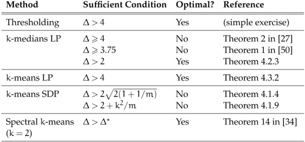
Table 1.1 summarizes the state of the art for recovery guarantees un-der the stochastic ball model. Theorem 1.4.3 is an improvement over [50], where it was shown that (k-medians lp), with high probability, recovers clusters drawn from the stochastic ball model provided the smallest dis-tance between ball centers is ∆_>3.75. We know that exact recovery only makes sense for ∆ > 2 (i.e., when the balls are disjoint). Once ∆ > 4, any two points within a particular cluster are closer to each other than any two points from different clusters, and so in this regime, cluster recovery follows from a simple distance thresholding.

Theorems 1.4.3 and 1.4.2 are tight in their dependence on the clus-ter separation ∆ and appear in [8]. Theorem 1.4.1 is proven through two different dual certificates, the first bound corresponds to the dual certificate from [8] and the second bound comes from the certificate from [34]. Neither of this bounds is tight and in some regimes the certificate from [8] gives a better guarantee than the certificate from [34] whereas in other regimes the opposite is true. The question of what is an optimal dual certificate re-mains open for this problem. An answer to this question could arise from comparing both certificates with the pre-certificate defined in [62].

Under the assumptions of the theorems above, popular heuristic al-gorithms such as Partitioning around Medoids (PAM) and Lloyd’s algorithm

(for k-medians and k-means, respectively) can fail with high probability. Even with arbitrarily large cluster separation, variants of Lloyd’s algorithm, such as k-means++ with overseeding by any constant factor, fail with high probability at exact cluster recovery. See Figure 1.6 for an illustration and [8] for details.

In our numerical experiments we observed that thek-medians linear program (k-medians lp) is often tight, even when the data points are drawn from a single spherical gaussian, were no cluster structure is expected. It re-mains an open problem to understand this phenomenon [10]. Thek-means semidefinite relaxation (k-means sdp) however, is not tight for more general data models, like mixtures of subgaussian distributions. In Section 1.4.4 we describe an algorithm that involves solving the SDP and rounding the

ob-Method Sufficient Condition Optimal? Reference

Thresholding ∆ > 4 Yes (simple exercise)

k-medians LP ∆_>4 No Theorem 2 in [27]

∆_>3.75 No Theorem 1 in [50]

∆ > 2 Yes Theorem 4.2.3

k-means LP ∆ > 4 Yes Theorem 4.3.2

k-means SDP ∆ > 2p2(1+1/m) No Theorem 4.1.4

∆ > 2+k2/m No Theorem 4.1.9

Spectralk-means ∆ > ∆? Yes Theorem 14 in [34] (k=2)

Table 1.1: Summary of cluster recovery guarantees under the stochastic ball model.

The second column reports sufficient separation between ball centers in order for the corresponding method to provably give exact recovery with high probabil-ity. The third column reports whether the sufficient condition on ∆ cannot be improved. Here,∆?=∆?(D,k)denotes the smallest value for which∆ > ∆? im-plies that minimizing the k-means objective recovers planted clusters under the (D,γ,n)-stochastic ball model with probability1−e−ΩD,γ(n)_{. In [34] we prove the}

Figure 1.6:Failure of Lloyd’s algorithm.

Recall the steps 1-3 in Lloyd’s algorithm. The output of the algorithm depends on its initialization. For example, let us say we want to cluster points drawn from the stochastic ball model, illustrated in this figure. If the initial guess has only one point from the two balls at the left and two points from the ball in the right, then Lloyd’s algorithm will fail to identify the correct clusters, obtaining an output similar to the one depicted in this figure. The probability of having a bad initial guess is positive and grows exponentially ink.

tained solution to a partition and we provide approximation guarantees for the algorithm.

1.4.3 Fast certification ofk-means optimality

On one hand we have very fast clustering algorithms like Lloyd’s [43] or manifold optimization based algorithms, whose solutions may be far from optimal. On the other hand we have optimization based algorithms like k-means SDP, which are slow but provide a certificate of optimality. What if we could combine the best of both worlds and obtain a fast algo-rithm with a certificate of optimality?

certifiably correct solutions to hard problems [9]. This technique leverages three components:

(i) A fast non-convex solver that produces the optimal solution with high probability (under some probability distribution of problem instances). (ii) A convex relaxation that is tight with high probability (under the same

distribution).

(iii) A fast method of computing a certificate of global optimality for the output of the non-convex solver in (i) by exploiting convex duality with the relaxation in (ii).

Using Bandeira’s technique in Chapter 5 we develop a quasi-linear time algorithm that provides certificates of k-means optimality of clusters [34], where (i) and (ii) are chosen to bek-means++ andk-means SDP respectively. In many useful applications thek-means SDP is not tight. In fact, in order for Bandeira’s technique to have practical value, we need to develop a robust version of it. In particular, a version that works even when the relaxation is not tight. This is an open problem that basically requires an algorithm that given an approximation solution of a convex optimization problem, it provably provides an approximate solution of the dual problem (faster than solving the dual problem).

The importance of this problem goes beyond clustering applications. It could provide a practical way of measuring the quality of solutions found by fast but maybe unreliable methods. For large datasets, problems tend to

be intractable for higher precision methods and this certificate can be of practical relevance.

1.4.4 Approximation guarantees

We earlier discussed that (k-means sdp), the semidefinite relaxation ofk-means, recovers the optimal clusters for the stochastic ball model. In Chapter 6 we study its performance under the general subgaussian mixture model, which includes the stochastic ball model and the Gaussian mixture model as special cases.

The semidefinite program is not typically tight under this general model, but the optimizer can be interpreted as a denoised version of the data and can be rounded in order to produce a good estimate for the centers (and therefore produce a good clustering).

To see this, let P denote the m×N matrix whose columns are the coordinates of the points we want to cluster: {xt,i}t∈[k],i∈[|At|]. Notice that whenever the semidefinite relaxation is tight,Xhas the form (1.8),

Xij=

1

|At| ifi,j∈At

0 otherwise (1.8)

then for each t ∈[k], PX has |At| columns equal to the centroid of points assigned toAt.

In particular, if Xisk-means-optimal, then PXreports thek -means-optimal centroids (with appropriate multiplicities). Next, we note that ev-ery SDP-feasible matrixX_>0satisfiesX>1=X1=1, and soX>is a

stochas-tic matrix, meaning each column ofPXis still a weighted average of columns from P. Intuitively, if the SPD relaxation (k-means sdp) were close to being tight, then the SDP-optimal Xwould make the columns ofPX close to the

k-means-optimal centroids. Empirically, this appears to be the case (see Figure 1.7 for an illustration). Overall, we may interpretPXas a denoised version of the original dataP, and we leverage this strengthened signal to identify good estimates for thek-means-optimal centroids.

What follows is a summary of our relax-and-round procedure for (approximately) solving thek-means problem (k-means):

Relax-and-roundk-means clustering procedure. Given andm×Ndata matrixP= [x₁· · ·x_N], do:

(i) Compute distance-squared matrix D defined by

Dij =kxi−xjk2₂.

(ii) Solve (k-means sdp), resulting in optimizerX. (iii) Cluster the columns of the denoised data matrix

PX.

For step (iii), we find there tends to bekvectors that appear as columns inPXwith particularly high frequency, and so we are inclined to use these as estimators for thek-mean-optimal centroids (see Figure 1.7, for example). Running Lloyd’s algorithm for step (iii) also works well in practice. To ob-tain theoretical guarantees, we instead find thek columns ofPXfor which the unit balls of a certain radius centered at these points inRm contain the

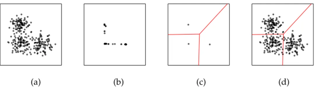
(a) (b) (c) (d)

Figure 1.7:Illustration of the relax and roundk-means clustering procedure (a) Draw 100 points at random from each of three spherical Gaussians over R2. These points form the columns of a2×300matrixP. (b)Compute the300×300 distance-squared matrixDfrom the data in (a), and solve thek-means semidefinite relaxation (k-means sdp) using SDPNAL+v0.3 [71]. (The computation takes about 16 seconds on a standard MacBook Air laptop.) Given the optimizerX, compute PXand plot the columns. We interpret this as a denoised version of the original dataP. (c) The points in (b) land in three particular locations with particularly high frequency. Take these locations to be estimators of the centers of the original Gaussians.(d)Use the estimates for the centers in (c) to partition the original data into three subsets, thereby estimating thek-means-optimal partition.

most columns of PX (see Theorem 6.5.1 for more details). An implemen-tation of our procedure is available on GitHub [67] and an interactive web visualization of the MNIST numerical simulation is available on [66].

In Chapter 6 we provide performance guarantees for the k-means semidefinite relaxation (k-means sdp) when the point cloud is drawn from a subgaussian mixture model. We adapt ideas from Guédon and Vershynin [32] and obtain approximation guarantees comparable with the state of the art for learning mixtures of Gaussians despite the fact that our algorithm is a generick-means solver and uses no model assumptions. In Section 6.5.1 we illustrate its numerical performance on the MNIST handwritten data set.

Recent work by Yan and Sarkar [70] adapted a similar version of our al-gorithm for kernel matrices and proved its strong consistency. They also prove that spectral methods are only weakly consistent, which provides some theoretical evidence of what we observe numerically: the semidefi-nite programming relaxation ofk-means performs much better than other algorithms at finding thek-means solution.

We summarize our approximation result in the following theorem Theorem 1.4.4. Given x1,. . .,xN points drawn independently from a mixture of

k subgaussian distributions in Rm. Say that the subgaussian a, for 1₆a₆k

has centerγa, andσ2 is an upper bound on the maximum covariance. Let∆min=

mina6=bkγa−γbkand similarly∆max. Ifkσ.∆min6∆max.Kσ, then we have

that there exists a permutationπon{1,. . .,k}such that

1 k k X i=1 kvi−γ˜π(i)k22.kK 2 σ2, (1.9)

where vi is what our algorithm chooses as the ith center estimate and γ˜a is the

average of the points sampled from the subgaussiana.

1.4.5 A polynomial-time relaxation for the Gromov-Hausdorff distance In the previous sections we have summarized how to use convex relaxations (i) to find exact solutions to clustering problems, (ii) to certify optimality of solutions acquired by faster but sometimes unreliable algo-rithms, and (iii) to provide approximate solutions with explicit

approxima-tion bounds via a relax and round procedure. Now we consider a different approach to optimization problems where we relax but do not round.

The Gromov-Hausdorff distance between finite metric spacesXand

Y, introduced in Section 1.2, can be formulated as an NP-hard optimization problem that for now we write in the abstract form (1.10). In Chapter 7 we consider a semidefinite relaxation of (1.10) obtaining a tractable optimiza-tion problem of the form (1.11).

d_GH(X,Y) :=minimize f_X,Y(z) (1.10) subject to z∈S.

˜

d_GH(X,Y) :=minimize f˜_X,Y(z) (1.11) subject to z∈S˜.

The relaxation (1.11) defines ˜d_GH, which we prove is a pseudomet-ric on point clouds and can be computed in polynomial time. We also show ˜dGH is a lower bound for the Gromov-Hausdorff distance dGH. Our

semidefinite relaxation (1.11) also providesz∈S˜ that can be interpreted as a relaxed correspondence between point clouds.

We study the topological properties of the relaxed pseudodistance ˜

d_GH (like convergence and compactness) and we observe that for almost every space X there exists a small local neighborhood where the metrics

d_GH and ˜d_GHare equivalent (see Corollary 7.2.8 and previous definitions). In Section 7.3 we exploit the theoretical observations to propose a non-convex optimization algorithm to approach the registration problem efficiently. The output of this algorithm not only provides a local opti-mum for the registration problem, but also an upper bound for the Gromov-Hausdorff distance.

The work in Chapter 7 appears in [68]. Note that a similar ver-sion to our SDP was recently introduced in [38] and further studied in [45] and [24]. Our work provides theoretical validation for some of the com-putational phenomena observed therein and complements their theoretical framework.

Chapter 2

Background

"The great watershed in optimization isn’t between linearity and nonlinearity, but convexity and nonconvexity."

– R. Tyrrell Rockafellar, in SIAM Review, 1993.

2.1

Optimization

In this section we present a small summary of optimization concepts we use in this thesis. For more comprehensive background information we refer the reader to the classic texts in convex optimization [51, 16] and [4] for manifold optimization.

Consider a general optimization problem of the form

minimize f_D(x) (2.1)

subject to x∈S.

When dealing with finite sets of data, we generally can formulate the prob-lems as a combinatorial optimization problem, whereSis a discrete set, and our problem consists of finding an optimal object among a finite set.

with specialized algorithms, but a large family of them, including the ones studied in this thesis, are NP-hard (and therefore one cannot expect to find an efficient algorithm that solves the problem in general). A useful strategy in this case is the relax-and-round paradigm introduced in Section 1.3.

In the convex optimization setting one relaxes the problem (2.1) to a minimization of a convex function over a convex set. In particular we focus in in linear programming (LP) and semidefinite programming (SDP). For LP the convex set considered is a convex polytope (i.e. the intersection of half spaces in Euclidean space). For SDP, the convex set is a spectahedron (i.e. the intersection of the cone of positive semidefinite matrices with an affine space). Both LP and SDP are particular cases of conic optimization, which we describe in Section 2.1.1. Conic optimization problems can be effi-ciently solved with interior point methods (and in general algorithms for LP tend to be more efficient than algorithms for SDP [51]). Conic optimization problems have an advantage with respect to generic convex optimization problems: conic problems have a dual problem that can be easily expressed in closed form. The dual problem is very useful to provide algorithms and theoretical results

A recently popular alternative to convex optimization is manifold optimization [4], where the setS is relaxed to a smooth convex manifold and the geometry of the manifold is exploited to obtain efficient algorithms. The main advantage of manifold optimization algorithms with respect to convex optimization is that for reasonably nice manifolds, manifold

opti-mization algorithms tend to run and converge much faster than interior point methods. The disadvantage is that in general they converge to local optima.

2.1.1 Cone programming

A setK⊂Rn is a cone ifx∈K implies tx∈K for allt_>0. LetK⊂

Rn _{and L⊂R}m _{be closed convex cones, consider c∈R}n_{, b∈R}m_{, and let}

A:Rn→Rmbe a linear operator. Then a cone programming problem is an optimization problem of the form (P).

minimize

x −hc,xi (P)

subject to b−Ax∈L x∈K

ForKclosed convex cone, we define its dual cone asK∗as

K∗:={y: hy,xi_>0 ∀x∈K}. Then the dual problem of (P) is defined as (D):

maximize

y −hb,yi (D)

subject to A∗y−c∈K∗ y∈L∗

where A∗ denotes the adjoint ofA, whileK∗ and L∗ denote the dual cones ofKandL, respectively.

In the optimization jargon we say that (P) is the primal problem and (D) is the dual problem. We say (P) has objective functionx7→−hc,xi, and a pointx∈Rn_{is said to be feasible for (P) if it satisfies the constraints in (P)} (i.e.b−Ax∈Landx∈K).

Proposition 2.1.1(Weak duality). Letxandybe feasible points for(P)and(D)

respectively. Then−hb,yi₆−hc,xi.

Proof. Sinceb−Ax∈Landy∈L∗then the definition of dual cone implies

0₆hb−Ax,yi=hb,yi−hA∗y,xi

then −hb,yi₆−hA∗y,xi. The same computation withx∈Kand A∗y−c∈

K∗gives−hA∗y,xi₆−hc,xiwhich gives the result.

Weak duality says that the dual problem provides lower bounds for the primal objective. Strong duality says that the optimal value of (P) actu-ally equals the optimal value of (D) (see [51] for a proof).

Theorem 2.1.2 (Strong duality). The problem (P) is feasible and has bounded optimal valueαif and only if (D)is feasible and has bounded optimal valueα.

2.1.1.1 Complementary slackness and dual certificates

Ifxand yare feasible for (P) and (D) respectively, weak duality im-plies

or equivalently, hc−A∗y,xi₆0₆hy,b−Axi. By strong duality, x and y

are optimal if and only if these inequalities are equal. That is,

hA>y−c,xi=0=hy,b−Axi.

In that sense, the primal variable x is complementary to the dual constraint A>y−cjust as the dual variable yis complementary to the pri-mal constraintb−Ax. These orthogonality relations are sometimes helpful when expressing the optimal y (called the dual certificate) in terms of the optimalx.

An interesting interpretation for the termdual certificateis that given

xfeasible for (P), if one can findyfeasible for (D) such that−hc,xi= −hb,yi

(or equivalentlyhA>y−c,xi=0=hy,b−Axi), thenyis a proof ofx’s opti-mality for (P).

2.1.2 Manifold optimization

Let us consider an optimization problem of the form

minimize f(Y) (2.2)

subject to Y∈M,

where f:M→ R is a smooth function and M is a compact Riemannian manifold.

For this kind of problems there is a beautiful theory [4] that allows us to think of the optimization problem (2.2) as an unconstrained optimization

where we replace the usual Euclidean ambient space by the Riemannian manifoldM.

The basic gradient descent algorithm relies on gradient and retrac-tion funcretrac-tions,

grad_f:M→T M, (2.3)

retrY :TYM→M. (2.4)

The gradient is computable using the Riemannian structure. The retraction is a choice of map which should satisfy

retrY(0) =0, d dt _t=0 retrY(tV) =V. (2.5) A canonical choice of retraction map is the exponential map forM, but this is not always computationally feasible. IfMis a submanifold of euclidean space,Y∈MandV∈TYM, then retrY(V)will be a first order approximation toY+V.

The algorithm consists of iteratively following the gradient offin the tangent space and then retracting back into the manifold:

Yn+1=retrYn(−αngradf(Yn)).

The stepsize αn can be set to be a small constant or adaptively chosen through a line search. Second order algorithms like trust regions have also been adapted to the manifold optimization setting [4].

In this thesis we restrict ourselves to first order methods, where gra-dient descent methods with backtracking Amijo line-search are proven to converge to a stationary point under mild hypotheses [13].

Theorem 6 in [13]. LetMa Riemannian manifold andf:M→Rbounded from below. Assume thatf◦retrY is Lipchitz with constantLindependent ofY. Then a gradient descent onMwith backtracking Amijo line-search initialized atY0returns

Y∗such that

f(Y∗)6f(Y0) and kgrad_f(Y∗)k6

Chapter 3

Manifold optimization techniques for

k

-means

clustering

3.1

The

k

-means manifold.

Recall our manifold optimization relaxation of k-means (3.1) intro-duced in Section 1.4.1

minimize Tr(DYY>) +λkY−k2F (3.1) subject to Y∈M,

whereλis a non-negative parameter,Y− indicates the negative entries ofY, andMis the submanifold

M={Y∈Rn×k: Y>Y=Ik, YY>1=1}. (3.2) The relaxation (3.1) is a constrained optimization where the set of constraints is a Riemannian manifold, so we can use the theory described in Section 2.1.2.

This chapter is based on the publication:

Timothy Carson, Dustin G. Mixon, Soledad Villar, Rachel Ward. Manifold optimization for k-means clusteringProceedings of the 2017 International Conference on Sampling Theory and Applications (SampTA), 2017 (to appear)

In order to implement the manifold optimization relaxation of k -means we need to explicitly construct the gradient and retraction maps (2.3) and (2.4). The tangent space toMatYis given by

TYM = {V ∈ Rn×k : V>Y + Y>V = 0,(VY> + YV>)1 = 0}. (3.3) Our manifold is a submanifold of a Euclidean space, and our objec-tive function is defined on the entirety of this Euclidean space. As such, we may compute the gradient of the objective function on our manifold by or-thogonally projecting its gradient in Euclidean space onto the tangent space to our manifold. That is, from the orthogonal projection ΠTYM :TYR

n×k _→

TYMwe can compute

gradM_f (Y) =ΠTYM◦ ∇f(Y)

where∇fis the gradient offin the ambient Euclidean spaceRn×k. For our objective function (with parameterλ),

fλ(Y) =Tr(DYY>) +λkY−k2, the gradient is computed in Section 3.2 to be

∇f_λ(Y) =2DY+2λ(Y)−. (3.4) In Section 3.3 we compute the orthogonal projection. It is:

ΠTYM(W) =W−2YΩ− (x1

where x= 1 nWY >_1∈Rn , Ω= 1 4(W >_Y+YW>_−2Y>_(x1>_+1x>_)Y)∈Rk×k . We use the following retraction:

retrY(V) =exp(B)exp(A0)Y, (3.6) where

A=Y>V∈Rk×k,

A0=YAY>∈Rn×n,

B=VY>−YV>−2A0∈Rn×n.

Here exp denotes the matrix exponential. We explain this retraction in Sec-tion 3.6.

3.2

Gradient of the objective function

We compute the ambient space gradient ∇fλ(Y)offλ. By definition we know∇fλ(Y) =Wif and only if for allV∈TYMwe have

hV,Wi=DYfλ(V) =Tr(D(VY>+YV>)) +λTr(V(Y>)−+ (Y−)V>) whereD_Yf_λ(V)is the directional derivative offλ. Equivalently,

Tr(WV>) =Tr(((D+D>)Y+2λ(Y−))V>). SinceDis symmetric we find (3.4).

3.3

Projection of a vector onto

T

Y

M

LetL1:Rn×k→Rk×ksymbeL1(W) =W>Y+Y>Wand letL2:Rn×k→Rn beL2(W) = (WY>+YW>)1. We can write the tangent space asTYM=ker(L) whereL=L1⊕L2:Rn×k→Rk×ksym×Rn.

We can use ker(L)⊥=im(L∗)to compute a parameterization for(TYM)⊥. Then we will solveW−L∗(Ω,x)∈ker(L) for (Ω,x) to find the projection

ΠTYM(W) =W−L

∗_(Ω,x).

We calculate that forΩsymmetric:

hL1W,Ωi=hW>Y,Ωi+hY>W,Ωi=hW>,ΩY>i+hW,YΩi=2hW,YΩi, from which we seeL∗₁Ω=2YΩ. Now calculate forx∈Rn_:

hL2W,xi=h(WY>+YW>)1,xi=hWY>+YW>,x1>i=hW,x1>Y+1x>Yi, soL∗₂x= (x1>+1x>)Y

Now we can findΩandxso thatW−L∗₁Ω−L∗₂x∈ker(L)by solving the system of equations:

L1(W−L∗1Ω−L∗2x) =0

L₂(W−L∗₁Ω−L∗₂x) =0

The first equation reads

W>Y+Y>W−4Ω−2Y>(x1>+1x>)Y=0

We can use this to substituteΩin the second equation to get:

where u= (In−YY>)WY>1 and B= −n(In−YY>). In particular we can choosexandΩas below (3.5). (There is nonuniqueness inxandΩbecause the image of L is not the full stated range, but of course the projection is unique.)

3.4

Homogenous structure of

M

Recall the Definition (3.2) ofM. LetM0be the manifold

M0={YY>:Y∈M}⊂Rn×nsym.

The manifoldM0 is the set of orthogonal projections onto akdimensional subspace of Rn including the vector 1n, and as such each member of M0 is determined by its image. A point in the manifoldM has the additional information of a choice of basis of the image ofX=YY>.

For a subspace A⊂ Rn_{, O(A) is the group of orthogonal matrices} for which Av=v for all v ∈A⊥. Let P ={1n}⊥ ⊂ Rn. We can see M as a homogenous space; it has a transitive action by O(P)×O(Rk)given by multiplication by the first factor on the left and theO(Rk)factor on the right:

M×O(P)×O(Rk)→M

(Y,Q,R)7→QYR.

The multiplication on the right by an element of O(Rk) controls changes which changeYbut notX, which may be seen directly from the computation

(YR)(YR)> =YRR>Y> =YY>. The multiplication on the left by Q∈O(P) allows for any change inX∈M0.

Multiplication ofY∈Mon the right byR∈O(Rk)is always equiva-lent to multiplication ofY on the left byR0=YRY>:

R0Y= (YRY>)Y=YR(Y>Y) =YR.

The matrix (YRY>)is an orthogonal projection onto im(X)composed with an orthogonal transformation of im(X), which may also be shown by com-puting

R0(I−X) =0, R(R0)> =X.

Recalling thatXis an orthogonal projection, the first equality shows thatR0

annihilates im(X)⊥and the second equality shows thatR0acts as an orthog-onal transformation of im(X)(on whichXis the identity).

For eachY₀the action byO(P)×O(Rk)has a stabilizer which is de-termined byX₀=Y₀Y₀>. This is due to redundancies of the right multiplica-tion in the left multiplicamultiplica-tion. The acmultiplica-tion byO(Rk)generates allY∈Mwith the sameX0:

{Y0R:R∈O(Rk)}={Y∈M:YY> =Y0Y0>}, but there are also elements ofO(P)which fixX₀namely,

{Q∈O(Rn) :QX0=X0Q,Q1n=1n}

3.5

Splitting the tangent space to

M

We may use our understanding of M as a homogenous space to compute a splitting of the tangent space TYM into two orthogonal parts; those which generate changes which fixX, and its perpendicular space. Let so(Rn)be the set of antisymmetric matrices inRn.

The matrices in{CY :C∈so(Rn)}which are tangent to the direction of fixedX(generated byO(im(X))⊕O(ker(X))) are

{C∈so(Rn) :CX=XC}.

This is the kernel of the linear mapso(n)→Rn×n_sym given byL(C) =CX−XC. The adjoint mapL∗:Rn×n_sym →so(n)is given byL∗(Ω) =ΩX−XΩ. Therefore

{C∈so(Rn) :CX=XC}⊥={ΩX−XΩ:Ω∈Rn×n_sym}.

GivenV∈TYMwe aim to writeV=BY+YAwhereA∈so(k),B∈so(P)and furthermoreB=ΩX−XΩforΩ∈Rn×n_sym. Under this ansantz, we compute

Y>V,VY>, andYV>and use thatY>Y=Ik to find

A=Y>V, (3.7)

B=ΩX−XΩ=VY>−YV>−2YAY>. (3.8) Using the formula forT_YM(3.3) one can check that we actually recoverVas

V=BY+YAand thatA∈so(Rk)andB∈so(P), i.e.

3.6

A retraction map

GivenV∈TYMwe aim to find a retraction retrY(V)∈M

satisfying (2.5). Write V as V =BY+YA as in (3.7), (3.8). Note we may also seeV asBY+ (YAY>)Y= (B+ (YAY>))Y; this is using the equivalence between multiplication on the right byO(Rk)and multiplication on the left byO(im(X)), mentioned in Section 3.4. LetA0=YAY>. Now set

retrY(V) =exp(B)exp(A0)Y. (3.10) The property (2.5) is straightforward given the differential equation satis-fied by exp, but it is not as obvious that ˜Y =retrY(V)∈M. The condition

˜

Y>Y˜ =Ifollows because we are performing left multiplication by orthogo-nal matrices. To check that ˜YY˜>1n=1nwe may compute,

(exp(B)exp(A0)Y)(exp(B)exp(A0)Y)>1n =exp(B)exp(A0)YY>exp(−A0)exp(−B)1n =exp(B)YY>exp(−B)1n

=exp(B)YY>1n=exp(B)1n=1n.

We have used, successively, that A0(YY>) = (YY>)A0=A0 (so exp(−tA0) commutes withYY>), thatB1n=0(so exp(−tB)fixes1n) and thatYY>1n=

1n. Note that the order of the matrix exponentials matters. For example,

V7→exp(A0)exp(B)YandV7→exp(B)Yexp(A) are paths satisfying (2.5) but will not lie on the manifold ifA016=0.

3.7

Numerical algorithm

The projection and retraction functions from the previous section al-low us to implement gradient descent algorithms in Manopt. In order to tackle the k-means problem, the algorithm we propose entails iteratively solving the manifold optimization relaxation of k-means (3.1), increasing the penaltyλuntil convergence to ak-means feasibleY. See Algorithm 1.

Algorithm 1: Manifold optimization iteration for k-means clus-tering 1: λ₀←0 2: repeat 3: Yn+1←GradientDescent(fλ)//Initialized atYn 4: λ_n+1←2λ_n+1 5: until kY₋k_F<

Theorem 6 in [13] guarantees that step 3 in the algorithm finds a sta-tionary point of the objective. The fact thatλTr(DYY>)is bounded forY∈M

suggests the algorithm may converge to a feasible clustering. It would be very interesting to show that Algorithm 1 converges to the actualk-means solution provided a good initialization.

3.8

Numerical simulations

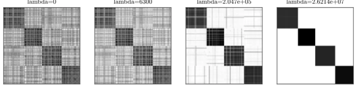
We sample points uniformly from 4 unit balls inR4with centers sep-arated by2.05 (following the stochastic ball model from Definition 1.4.1). We sample 22, 18, 19 and 21 points from each ball respectively. We run Algorithm 1 using Manopt to implement step 3. In Figure 3.1 we plot the

lambda=0 lambda=6300 lambda=2.047e+05 lambda=2.6214e+07

Figure 3.1:Illustration ofYYT for iterations of Algorithm 1 with successive values ofλ.

Note the first image is equivalent to a purely spectral method while the last im-age coincides with the planted solution of thek-means problem. The algorithm is oblivious to the planted order of points. We choose the order where the first points belong to the first cluster, and so on, to simplify visualization.

results.

3.9

Discussion

Before manifold optimization became popular, Burer and Monteiro [20] introduced the idea of using a low rank factorization of a matrix in order to solve a semidefinite program of the form.

minimize Tr(CX) (3.11)

subject to Tr(AiX) =bi16i6m, X0

According to the Pataki bound [55], the solution of (3.11) is a matrixX=YY>

for some Y ∈Rn×p with p(p+1)₂ 6m. Therefore if we replace the positive semidefinite constraint in (3.11) by X=YY> for Y∈Rn×p the global mini-mizer of both problems coincide. In their paper, Burer and Monteiro pro-pose an augmented lagrangian iteration in X=YY>. They prove it verges to a stationary point of their objective. Since the objective is not

con-vex there is a priori no guarantee that it won’t converge to some spurious stationary point.

Later work by Journée and collaborators [37] introduced a manifold optimization algorithm and proved that, under somewhat restrictive con-ditions (not satisfied by our clustering problem), it converges to the global optimizer.

Recent work by Boumal, Voroninski and Bandeira [15] extend Journée’s work by showing that the Bourer-Monteiro problem (i.e. the minimization in matrices of the formYY>) is equivalent to respective SDP for some spe-cific problems. They actually show that for those problems there are no spurious stationary points.

Some natural questions arise: (a) How small can pbe chosen with still no spurious stationary point? In their original paper Burer and Mon-teiro suggested that if the rank of the planted solution is kone should be able to choose p=k+1 orp=k+2. (b) Is it possible to adapt manifold optimization methods to singular manifolds? And in particular, (c) can a theory like this be developed for manifolds with boundary?

To the best of our knowledge the best algorithms that can deal ef-ficiently and reliably with semidefinite programs with non-negative con-straints are based on interior point methods [51]. As far as we know, there is no theory that provides convergence guarantees for matrix factorization based algorithms in presence of non-negative constraints; nor even

suc-cessful implementation for algorithms like that for generic SDPs with non-negative constraints.

Chapter 4

Finding the exact solution: tightness in convex

optimization

4.1

A semidefinite program relaxation for

k

-means

Recall Peng and Wei’s semidefinite relaxation (k-means sdp) of the

k-means problem (k-means). minimize

X∈RN×N

1

2trace(DX) (k-means sdp)

subject to X1=1, trace(X) =k, X_>0, X0.

In this section we show (k-means sdp) is typically tight under the stochastic ball model. We do it in two different ways, one appears in [8] and the other one in [34]. The basic idea is (i) to find a deterministic condition on the set

This chapter is based on two publications:

Pranjal Awasthi, Afonso S. Bandeira, Moses Charikar, Ravishankar Krishnaswamy, Soledad Villar, Rachel Ward. Relax, no need to round: Integrality of clustering formulations.

Proceedings of the 2015 Conference on Innovations in Theoretical Computer Science, pp. 191-200. ACM, 2015.

Takayuki Iguchi, Dustin G. Mixon, Jesse Peterson, Soledad Villar.Probably certifiably correct k-means clusteringMathematical Programming, 2016 (to appear).

In both of the papers the author contributed in developing the main ideas of the paper, the mathematical proofs and numerical experiments.

of points under which the relaxation finds the k-means-optimal solution, and (ii) to discuss when this deterministic condition is satisfied with high probability under the stochastic ball model.

To find the dual program to (k-means sdp) we leverage the cone pro-gramming theory from Section 2.1.1. In our case, c= −D, x=X, and K is simply the cone of positive semidefinite matrices (as isK∗). Before we deter-mineL, we need to interpret the remaining constraints in (k-means sdp). To this end, we note that Tr(X) =kis equivalent tohX,Ii=k,X1=1is equiva-lent to having X,1 2(ei1 > +1e>_i ) =1 ∀i∈{1,. . .,N}, andX_>0is equivalent to having

X,1 2(eie > j +eje>i ) >0 ∀i,j∈{1,. . .,N}, i₆j.

(These last two equivalences exploit the fact thatXis symmetric.) As such, we can express the remaining constraints in (k-means sdp) using a linear operator Athat sends any matrix Xto its inner products with I, {1₂(ei1>+

1e>_i )}N_i=1, and{1₂(eie>_j +eje>_i )}N_i,j=1,i6j. Note that the remaining constraints in (k-means sdp) are equivalent to havingb−Ax∈L, whereb=k⊕1⊕0and

L=0⊕0⊕RN(N+1)/2_>0 . Writingy=z⊕α⊕(−β), the dual of (k-means sdp) is then given by

minimize z∈R,α∈RN_,β∈RN×N kz+ N X i=1 αi (k-means sdp dual) subject to Q:=zI+ N X i=1 α_i·1 2(ei1 >_+1e> i ) − N X i=1 N X j=i β_ij·1 2(eie > j +eje>i ) +D0 β_>0

For notational simplicity, from this point forward, we organize in-dices according to clusters. For example,1ashall denote the indicator func-tion of the ath cluster. Also, we shuffle the rows and columns ofX and D

into blocks that correspond to clusters; for example, the(i,j)th entry of the (a,b)th block of Dis given byD(a_ij,b). We also indexαin terms of clusters; for example, the ith entry of the ath block ofα is denotedαa,i. For β, we

identify β:= N X i=1 N X j=i βij· 1 2(eie > j +eje>i ).

Indeed, wheni₆j, the(i,j)th entry ofβisβij. We also considerβas having its rows and columns shuffled according to clusters, so that the(i,j)th entry of the(a,b)th block isβ(a_ij,b).

With this notation, the following proposition characterizes all possi-ble dual certificates of (k-means sdp):

Proposition 4.1.1. Take X:= Pk_a=1n1 a1a1

>

a, where na denotes the number of

points in clustera. The following are equivalent:

(b) Every solution to the dual program(k-means sdp dual)satisfies

Q(a,a)1=0, β(a,a)=0 ∀a∈{1,. . .,k}.

(c) Every solution to the dual program(k-means sdp dual)satisfies

αa,r= − 1 na z+ 1 n2 a 1>D(a,a)1− 2 na e>_rD(a,a)1 ∀a∈{1,. . .,k}, r∈a.

Proof. (a)⇔(b): By complementary slackness, (a) is equivalent to having both hA∗y−c,Xi=0 (4.1) and hy,b−A(X)i=0. (4.2) SinceQ0, we have hA∗y−c,Xi=hQ,Xi= Q, k X t=1 1 nt 1t1>t = k X t=1 1 nt 1>_tQ1t>0,

with equality if and only ifQ1a =0 for everya∈{1,. . .,k}. Next, we recall thaty=z⊕α⊕(−β),b−A(X)∈L=0⊕0⊕RN(N+1)/2_>0 , andb=k⊕1⊕0. As such, (4.2) is equivalent to βhaving disjoint support with {hX,1₂(eie>_j +

eje>_i )i}N_i,j=1,i6j, i.e.,β(a,a)=0for every clustera.

(b)⇒(c): Take any solution to the dual SDP (k-means sdp dual), and note that Q(a,a)=zI+ Xk t=1 X i∈t αt,i· 1 2(et,i1 >_+1e> t,i) (a,a) −β(a,a)+D(a,a) =zI+X i∈a αa,i· 1 2(ei1 >_+1e> i ) +D (a,a) , (4.3)

where the 1 vectors in the second line are na-dimensional (instead of N -dimensional, as in the first line), and similarly for ei (instead of et,i). We

now consider each entry ofQ(a,a)1, which is zero by assumption:

0=e>_r Q(a,a)1 =e>_r zI+X i∈a αa,i· 1 2(ei1 >_+1e> i ) +D(a,a) 1 =z+X i∈a αa,i· 1 2(e > rei1>1+e>r1e>i 1) +e>rD(a,a)1 =z+X i∈a αa,i· 1 2(naδir+1) +e > rD(a,a)1. (4.4) As one might expect, these na linear equations determine the variables

{αa,i}i∈a. To solve this system, we first observe

0=1>Q(a,a)1 =1> zI+X i∈a αa,i· 1 2(ei1 >_+1e> i ) +D(a,a) 1 =naz+ X i∈a αa,i· 1 2(1 >_e i1>1+1>1ei>1) +1>D(a,a)1 =naz+na X i∈a αa,i+1>D(a,a)1, and so rearranging gives

X i∈a αa,i= −z− 1 na 1>D(a,a)1.