Bayesian ranking and selection methods using hierarchical mixture models in microarray studies.

(1)

Title Bayesian ranking and selection methods using hierarchical_{mixture models in microarray studies.}

Author(s) Noma, Hisashi; Matsui, Shigeyuki; Omori, Takashi; Sato,_Tosiya

Citation Biostatistics (2010), 11(2): 281-289

Issue Date 2010-04

URL http://hdl.handle.net/2433/139478

Right © The Author 2009. Published by Oxford University Press.; 許_{諾条件により本文は2011-05-01に公開}

Type Journal Article

Textversion author

(2)

Biostatistics (2010), 11, 2, pp. 281-289 doi: 10.1093/biostatistics/kxp047

Bayesian ranking and selection methods

using hierarchical mixture models in microarray studies

HISASHI NOMA

Department of Biostatistics, Kyoto University School of Public Health Yoshida Konoe-cho, Sakyo-ku, Kyoto 606-8501, Japan

SHIGEYUKI MATSUI

Department of Data Science, The Institute of Statistical Mathematics 10-3 Midori-cho, Tachikawa, Tokyo 190-8562, Japan

TAKASHI OMORI, TOSIYA SATO

Correspondence: Hisashi Noma

Phone +81-75-753-9466 FAX +81-75-753-4487

e-mail: [email protected]

(3)

Summary

The main purpose of microarray studies is screening to identify differentially expressed genes as candidates for further investigation. Because of limited resources in this stage, prioritizing or ranking genes is a relevant statistical task in microarray studies. In this article, we develop three empirical Bayes methods for gene ranking on the basis of differential expression, using hierarchical mixture models. These methods are based on (1) minimizing mean squared errors of estimation for parameters, (2) minimizing mean squared errors of estimation for ranks of parameters, and (3) maximizing sensitivity in selecting prespecified numbers of differential genes, with the largest effect. Our methods incorporate the mixture structures of differential and non-differential components in empirical Bayes models to allow information borrowing across differential genes, with separation from nuisance, non-differential genes. The accuracy of our ranking methods is compared with that of conventional methods through simulation studies. An application to a clinical study for breast cancer is provided.

Key words:empirical Bayes; gene expression; hierarchical mixture models; microarrays;

(4)

1

1. Introduction

Recent developments in gene expression microarrays have enabled comprehensive screening of differentially expressed genes between different clinical subclasses. In genome-wide studies with microarrays, multiple testing is widely adopted, and statistically significant genes are reported as candidate genes for further investigation. Because of limited resources at this stage, prioritizing or ranking genes is needed.

There are at least two criteria on which genes are ranked; one is related to the probability of non-differential expression, the other is to the magnitude of differential expression or the strength of association with the clinical outcome. An example of the former criterion is the local false discovery rate, which represents the posterior

probability of non-differential expression of each gene (Efron and others, 2001; Efron,

2008). A similar or related statistic using hierarchical Bayes models was derived and

discussed by Newton and others (2004). The ranking based on the local false discovery

rate is optimal for selecting differentially expressed genes from the viewpoint of

Bayesian decision theory (Berger, 1985; McLachlan and others, 2006).

For the latter criterion regarding magnitude of association, the fold change—which corresponds to the ratio or difference of mean expression levels between different clinical

subtype classes—is commonly used (McLachlan and others, 2004; Guo and others,

2006; Choe and others, 2005). Some authors have reported that gene ranking based on

the fold change is reproducible (MAQC Consortium, 2006) and accurate for large

absolute changes in gene expression (Witten and Tibshirani, in preparation1). However,

the accuracy of gene ranking can be improved by ―borrowing strength‖ across genes. Specifically, the ranking of empirical Bayes estimators can be more accurate than that of

1

(5)

2

conventional statistics such as maximum likelihood estimators (Laird and Louis, 1989). Laird and Louis (1989) and Shen and Louis (1998) discussed optimal ranking in

empirical Bayes inference. Lin and others (2006) discussed various loss functions in

Bayesian optimal ranking and selection rules, and derived optimal rules for selecting top-ranked features.

An important feature of microarray data is that a large proportion of the genes investigated are non-differential. The incorporation of this feature of microarray data could allow for information-sharing across differential genes separated from nuisance, non-differential genes. In this article, we propose empirical Bayes methods for gene ranking on the basis of the strength of association under structural models that reflect this feature. Specifically, we assume a hierarchical mixture model with a two-stage compound sampling model, in which the second stage of the model is a mixture distribution of differential and non-differential components (Newton and Kendziorski, 2003; Lönnstedt

and Speed, 2002; Gottardo and others, 2003).

We present the framework of the hierarchical mixture modeling and its empirical Bayes inference in Section 2 and develop three ranking and selection rules in Section 3. In Section 4, we compare the proposed rules with conventional or other methods through simulations. We describe the application to a breast cancer clinical study in Section 5. Discussion is provided in Section 6.

(6)

3

2. Hierarchical mixture modeling

The gene expression data considered here comprise normalized log ratios from two-color cDNA arrays or normalized log signals from oligonucleotide arrays (e.g., Affymetrix GeneChip). We consider a two-class comparison problem: a binary response—e.g., a poor prognosis and good prognosis, is compared on the basis of the expression levels of

m candidate genes from n samples. For gene j, let θj be the parameter of interest, i.e., the

difference in the mean expression level between the two classes (j = 1, …, m). As an

estimator of θj, let Yj be the fold change, which is the difference in the sample mean

expression level obtained from n samples (Guo and others, 2006; Choe and others, 2005).

We consider a two-stage model with i.i.d. sampling from a three-component mixture prior

and from a normal gene-specific sampling model:

Yj | θj ~ N(θj, σj2) (2.1)

θj ~ π0δ(θ) +π1g1(θ |ξ1) + π2 g2(θ |ξ2).

Here, δ(θ) is the Dirac delta function, representing non-differential expression between

two classes. The density functions g1(θ |ξ1) and g2(θ |ξ2) correspond to the non-null

components of under-expression and over-expression, respectively, for a particular class,

e.g., poor prognosis. The proportion πi represents the mixing proportion (i = 0, 1, 2), with

π0 + π1 + π2 = 1. In the first-stage model in (2.1), we assume that the gene-specific

variance σj2 is known. We denote Zij(i = 0,1,2; j = 1,2,…,m) as unobservable indicator

random variables, such that Zij = 1 if gene j belongs to the i-th component, and Zij = 0

otherwise. The πi (i = 0,1,2) correspond to the probability of Zij = 1. An estimate of the

hyperparameter η = (π0, π1, ξ1, ξ2) can be obtained by maximizing the marginal likelihood

(7)

4

(Dempster and others, 1977) to cope with the unobservable indicator variable Zij in the

mixture model. The hyperparameters of interest, i.e., ξ1 and ξ2 in the distribution of the

effect sizes j, can be estimated more stably by using fixed or, more generally,

constrained estimates of the mixing proportions or by introducing prior distributions on

the mixing proportions in the EM algorithm (e.g., Gottardo and others, 2003; Newton

and others, 2001; Newton and others, 2004; Lo and Gottardo, 2007). In this article, we

consider the former strategy and adopt a two-stage procedure that estimates π0 as in

Storey (2002) and treat this estimate as a fixed value in the EM algorithm. We assume

conjugate normal distributions N(μ1, τ12) and N(μ2, τ22) (μ1 > 0, μ2 < 0) for g1(θ| ξ1) and

g2(θ| ξ2), respectively.

3. Posterior inference

For simplicity, our discussion here is restricted to identifying genes with the greatest

positive θj, i.e., overexpressed genes for a particular class. Its extension to the two-sided

version—to obtain genes with the greatest absolute θj for both over-expressed and

under-expressed genes—is straightforward.

3.1. Rankingbased on posterior mean (PM)

From model (2.1), we obtain the posterior distribution:

where p0j, p1j, and p2j are the posterior densities of each component, which are obtained as

(8)

5            2 2 2 2 2 2 2 2 , N j i j i j i i j j i σ τ σ τ σ τ μ σ y τ , (i = 1,2)

respectively. The posterior probability that gene j belongs to the i-th component (i =

0,1,2) is ) | ( ) | ( ) ( ) | ( ) | 1 Pr( 2 2 2 1 1 1 0 0 ξ ξ ξ j j j j j j i j ij i j ij y h π y h π y h π y h π y Z     _. _(3.1)

Here, h0j, h1j, and h2j are the marginal densities of the Yjs, in each component, namely N(0,

σj2), N(μ1, σj2 + τ12), and N(μ2, σj2 + τ22) for i = 0,1,2, respectively.

Minimizing the squared error loss, the Bayes estimator of θj is the posterior mean

(Carlin and Louis, 2000). For the hierarchical mixture model, the posterior mean is obtained as

+ Pr(Z2j = 1| yj) E[θj|Z2j = 1,Yj] . (3.2)

This is the weighted average of the posterior means of each component, where the weights are the posterior probabilities of component membership (3.1). The ranking is thus obtained via the magnitude of the posterior means (the ‗PM‘ method).

3.2. Ranking based on rank posterior means (RPM)

If the ranks of the parameters are the target feature, using the rank estimator is more appropriate than using the parameter estimator (Laird and Louis, 1989; Shen and Louis, 1998; Louis and Shen, 1999). We consider ranking within differential genes with positive effects, defined as



   m k k j k j j Z Z I θ θ R 1 1 1 ( ) ,

(9)

6

where Rj has a large value when gene j belongs to the non-null component with positive

effect and has a large θjvalue, or is 0 when gene j belongs to the other components. For

the squared error loss, the Bayes estimator of Rj is the posterior mean:



     m k k j k j j k j j j j y Z y Z y θ θ y y R E 1 1 1 1| ) Pr( 1| )Pr( | , ) Pr( ] | [ . (3.3)

Thus, gene ranking is obtained by the rank posterior means (the ‗RPM‘ method).

3.3. Rankingbased on tail-area posterior probability (TPP)

Because of the limited resources available in subsequent studies, the number of selected

genes may be prespecified as a small number, K (Matsui and others, 2008). In this

situation, we consider the K genes with the greatest positive effects as the target. Lin and

others (2006) provided various loss functions and derived optimal ranking and selection rules via Bayesian decision theory; we generalize their rank-based misclassification loss

function that equivalently penalizes to misclassifications between the true top K ranked

genes and other the differential genes:







   m j est j j est j j est R R K FN R R K FP m R R K L 1 1 / 0 ( , , ) ( , , ) 1 ) , , ( , where FP(K, Rj, Rjest) = I{Rj ≤ m1 – K, Rjest > m1 – K} FN(K, Rj, Rjest) = I{Rj > m1 – K, Rjest ≤ m1 – K} .

The Rjest are estimators of the Rj, and m1 = ∑j Z1j is the number of genes generated from

the non-null component with positive effects in the m measured genes.

The derived optimal rule is to select K genes which have large values of

(10)

7

as in Lin and others (2006). However, it is difficult to obtain the posterior distribution of

Rj and to calculate j(K) directly. Instead, we can use a simple computable approximation

of j(K). Define γ = K / (m1+1) and let G1 be the cumulative distribution function of g1.

Under the similar conditions of Theorem 5 described in Lin and others (2006), the

approximation of j(K) is obtained as ) | 1 Pr( ) , 1 | ) ( Pr( ) ( *_j K  θ_j G₁1 γ Z₁_j  y Z₁_j  y P , (3.4) where



       _m j j j m j j j j j j y Z y Z y z t θ t G 1 1 1 1 1 1 ) | 1 Pr( ) | 1 Pr( ) , 1 | Pr( ) ( .

P*j(K) corresponds to the tail-area posterior probability of θj. Proof of this approximation

is provided in the Supplementary Material. Here, we denote this rule as the ‗TPP

(tail-area posterior probability‘ method. The quantity m1 can be replaced by its estimator

∑j Pr(Z1j = 1|yj) (McLachlan and others, 2004).

4. Simulation studies

We conducted a series of simulation studies to assess the performance of our proposed methods. Details of the simulations are presented in Section A of the Supplementary

Material available at Biostatistics online.

In summary, the sensitivity and root mean squared error (RMSE) of all the proposed methods were better than those of the other methods. As was expected, the TPP method had the greatest sensitivity, the RPM method had the lowest RMSE values, and the posterior probability of differentially expressed (PPDE) (3.1) ranking had the lowest false

(11)

8

positive rate. The posterior mean under unimodal hierarchical model (PMU) method,

which lacks mixture components, had a lower sensitivity and a larger RMSE, compared with the PM method. The fold change had comparable sensitivity and RMSE values for large sample sizes, but not for small sample sizes. The fold change had very large false positive rates even when the sample size was large, because it does not guard against selecting null genes.

5. Application to a breast cancer study

We illustrate the proposed methods using the dataset from a breast cancer clinical study

(Wang and others, 2005). The data are available from the NCBI GEO database

(GSE2034). This study was a large Affymetrix-based gene expression profiling study of 286 untreated patients with lymph-node-negative primary breast cancer, and analyzed estrogen receptor positive and negative patients separately. Here, we restrict our attention to the estrogen receptor positive patients. In this study, out of 22,283 genes, 60 genes were selected on the basis of statistical significance for predicting the risk of relapse. We considered comparison of patients who were relapse-free at five years (good prognostic group) and the other patients (poor prognostic group). During the follow-up period, of the 204 estrogen receptor positive patients, 138 patients were relapse-free at five years, whilst 66 developed distant metastasis.

The hyperparameters were estimated as πˆ0 0.769 , πˆ1 0.055 , πˆ2 0.176 ,

182 . 0 ˆ₁ 

μ , τˆ₁2 0.0212, μˆ₂ 0.149 , τˆ₂2 0.0142. The σj2 were estimated on a

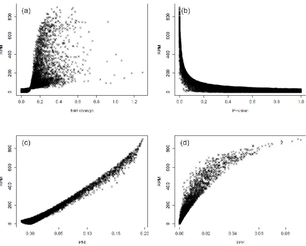
gene-by-gene basis assuming a common variance between the two prognostic groups. Figure 1 represents comparison between the RPM statistic, which was shown to yield

(12)

9

good gene ranking in the simulation studies in Section 4, and the other statistics for overexpressed genes in the poor prognostic group. Similar trends were observed in underexpressed genes for the poor prognostic group. Figure 1(a) indicates substantial discrepancy in gene ranking between the RPM statistic and the fold change. In Figure

1(b), top ranked genes based on the RPM statistics had the smallest P-values, but

low-ranked genes using the RPM statistic could also have very small P-values. Figures

1(c) and (d) indicate good agreement of gene ranking among the PM, RPM, and TPP statistics, especially, for the greatest values of these statistics (i.e., for top-ranked genes). For example, out of top 30 genes based on the RPM statistic, 27 and 21 genes were also selected in top 30 genes based on the PM and TPP statistics, respectively. The discrepancy in gene ranking between the proposed methods and fold change in Figure 1(a) would reflect very high false positive rates for fold change as we found in our simulation study.

We also investigated overlap of top genes between the proposed methods and the 60 genes reported in the original paper (see Section B of the Supplementary Material at

Biostatistics online). There were 7 overlaps when the top 30 genes were selected by the RPM method for each of overexpression and underexpression in the poor prognostic group. 26 (43%) of the 60 genes reported in the original paper were amongst the top 1% of genes according to their RPM values. As indicated by Figure 1(b), there were fewer

overlaps between the proposed methods and the t-statistic. Because the sensitivity of the

proposed methods was higher, gene ranking based on the proposed methods would be more reliable.

(13)

10

6. Discussion

In microarray studies, prioritizing or ranking genes is an important statistical task. Because the number of simultaneous comparisons can go into the tens of thousands, gene ranking can suffer from a lack of accuracy. Sharing information across genes and incorporating the null/non-null mixture structure are expected to be effective in improving accuracy. As seen in our simulations, the proposed PM, RPM, and TPP methods showed higher sensitivity and lower error of rank estimation for differential genes with the greatest effects, compared to conventional methods. In addition, these methods had low false positive rates. Although the results of our resampling studies indicated that such good performance can be compromised by violating the model assumptions, including independence among genes and the normality of gene expressions, our ranking methods, especially the RPM method, were still accurate compared to the other methods. Violation of normality can be handled by using other parametric distributions, as noted in Section 2. The greater accuracy of the PM method, compared to

the PMU method, shows that incorporating the null-mixture component is effective in

improving ranking accuracy. The PPDE ranking had the lowest false positive rate, as was

expected because of its theoretical optimality (Berger, 1985; McLachlan and others,

2006). These results are reasonable because a ranking method performs well for the criterion or loss function in gene ranking from which it is derived. Ranking methods should be selected according to the criterion of interest in gene ranking, i.e., depending on the probability of non-differential expression or the magnitude of differential expression.

(14)

11

good performance in sensitivity and RMSE of gene ranking under large sample scenarios

(n/2 = 80) in the simulations described in the Supplementary Material. Further, the RMSE

of fold change was lower than the proposed empirical Bayes methods under large sample scenarios in the resampling exercise in the Supplementary Material. A similarly good performance using conventional methods, compared to those of empirical Bayes methods, has also been seen with large samples in other experiments (Greenland, 1993). In small sample scenarios, however, optimality was largely violated. Further, with respect to false positive rates, the ranking of the fold change did not perform well, even with large samples. Although the MAQC project (MAQC Consortium, 2006) reported good reproducibility of ranking based on fold change, ―accuracy‖ and ―reproducibility‖ are different concepts as remarked by Witten and Tibshirani (in preparation). Hence, ranking via the fold change is not recommended for general use when the objective is to prevent false positive detection.

For general practical use, the proposed three methods should be used according to the purpose of analysis. However, for the three proposed methods, the sensitivities in detecting differential genes with the greatest effects as well as the false positive rates were comparable. Accordingly, we would recommend the RPM method.

As noted in Section 2, attempts to obtain stable estimates of the hyperparameters of

interest, i.e., ξ1 and ξ2 in the distribution of the effect sizes j, include the use of

reasonable estimates of the mixing proportions such as treating π0 as fixed quantities,

invoking reasonable constraints or placing prior distributions on the mixing proportions in the EM algorithm. Comparison of these approaches is outside the scope of this paper, but it is an important subject for future research.

(15)

12

The R code for gene ranking is available in the Supplementary Material at

Biostatistics online.

Supplementary Material

Supplementary material is available at http://biostatistics.oxfordjournals.org.

Acknowledgements

The authors would like to thank Tomonori Oura for many valuable comments and advice on an earlier draft of this article, and the editor for helpful comments and suggestions.

(16)

13

References

Berger, J. O. (1985). Statistical Decision Theory and Bayesian Analysis, New York:

Springer.

Carlin, B. P. and Louis, T. A. (2000). Bayes and Empirical Bayes Methods for Data

Analysis. New York: Chapman & Hall.

Choe, S. E., Boutros, M., Michelson, A. M., Church, G. M. and Halfon, M. S. (2005). Preferred analysis methods for Affymetrix GeneChips revealed by a wholly defined

control dataset. Genome Biology6, R16.

Dempster, A. P., Laird, N. M. and Rubin, D. B. (1977). Maximum likelihood from

incomplete data via the EM algorithm (with discussion). Journal of the Royal

Statistical Society, Series B 39, 1–38.

Efron, B., Tibshirani, R., Storey, J. and Tusher, V. (2001). Empirical Bayes analysis of a

microarray experiment. Journal of the American Statistical Association 96,

1151–1160.

Efron, B. (2008). Microarrays, empirical Bayes and the two-groups model (with

discussion). Statistical Science23, 1–47.

Gottardo, R., Pannucci, J. A., Kuske, C. R. and Brettin, T. (2003). Statistical analysis of

microarray data: a Bayesian approach. Biostatistics4, 597–620.

Greenland, S. (1993). Methods for epidemiologic analyses of multiple exposures: A review and comparative study of maximum-likelihood, preliminary testing, and

empirical-Bayes regression. Statistics in Medicine12, 717–736.

Guo, L., Lobenhofer, E. K., Wang, C., Shippy, R., Harris, S. C., Zhang, L., Mei, N., Chen, T., Herman, D., Goodsaid, F. M., Hurban, P., Phillips, K. L., Xu, J., Deng, X. T., Sun,

(17)

14

Y. M. A., Tong, W. D., Dragan, Y. P. and Shi, L. M. (2006). Rat toxicogenomic study

reveals analytical consistency across microarray platforms. Nature Biotechnology24,

1151–1161.

Laird, N. M. and Louis, T. A. (1989). Empirical Bayes ranking methods. Journal of

Educational Statistics 14, 29–46.

Lin, R., Louis, T. A., Paddock, S. M. and Ridgeway, G. (2006). Loss function based

ranking in two-stage, hierarchical models. Bayesian Analysis1, 915–946.

Lo, K. and Gottardo, R. (2007). Flexible empirical Bayes models for differential gene

expression. Bioinformatics23: 328–335.

Lönnstedt, I. and Speed, T. P. (2002). Replicated microarray data. Statistica Sinica 12,

31–46.

Louis, T. A. and Shen, W. (1999). Innovations in Bayes and empirical Bayes methods:

estimating parameters, populations and ranks. Statistics in Medicine18, 2493–2505.

MAQC Consortium (2006). The MicroArray Quality Control (MAQC) project shows

inter- and intraplatform reproducibility of gene expression measurements. Nature

Biotechnology24, 1151–1161.

Matsui, S., Zeng, S., Yamanaka, T. and Shaughnessy, J. (2008). Sample size calculations

based on ranking and selection in microarray experiments. Biometrics64, 217–226.

McLachlan, G. J., Bean, R. W. and Jones, L. B.-T. (2006). A simple implementation of a normal mixture approach to differential gene expression in multiclass microarrays.

Bioinformatics22, 1608–1615.

McLachlan, G. J., Do, K. -A. and Ambroise, C. (2004). Analyzing Microarray Gene

(18)

15

Newton, M. A., Kendsiorski, C. M. (2003). Parametric empirical Bayes methods for

microarrays. In Parmigiani, G., Garrett, E. S., Irizarry, R. A. and Zeger, S. (eds), The

Analysis of Gene Expression Data: Methods and Software. New York: Springer, pp. 254–271.

Newton, M. A., Kendziorski, C. M., Richmond, C. S., Blattner, F. R. and Tsui, K. W. (2001). On differential variability of expression ratios: Improving statistical

inference about gene expression changes from microarray data. Journal of

Computational Biology8: 37–52.

Newton, M. A., Noueiry, A., Sarkar, D. and Ahlquist, P. (2004). Detecting differential

gene expression with a semiparametric hierarchical mixture method. Biostatistics 5,

155–176.

Shen, W. and Louis, T. A. (1998). Triple-goal estimates in two-stage hierarchical models.

Journal of the Royal Statistical Society, Series B 60, 455–471.

Storey, J. D. (2002). A direct approach to false discovery rates. Journal of the Royal

Statistical Society, Series B 64, 479–498.

Wang, Y., Klijn, J. G., Zhang, Y., Sieuwerts, A. M., Look, M. P., Yang, F., Talantov, D., Timmermans, M., Meijer-van Gelder, M. E., Yu, J., Jatkoe, T., Berns, E. M., Atkins, D. and Foekens, J. A. (2005). Gene-expression profiles to predict distant metastasis

(19)

Figure 1. Comparison of the RPM statistic with other statistics for the breast cancer dataset. The four panels show scatter plots of the RPM statistic versus the fold change (a),

the P-values from two-sample t-tests (b), the PM statistic (c), and the TPP statistic with K