Selected topics in measurement error and functional data analysis

(1)

2016

Selected topics in measurement error and

functional data analysis

Yuhang Xu

Iowa State University

Follow this and additional works at:https://lib.dr.iastate.edu/etd Part of theBiostatistics Commons

This Dissertation is brought to you for free and open access by the Iowa State University Capstones, Theses and Dissertations at Iowa State University Digital Repository. It has been accepted for inclusion in Graduate Theses and Dissertations by an authorized administrator of Iowa State University Digital Repository. For more information, please [email protected].

Recommended Citation

Xu, Yuhang, "Selected topics in measurement error and functional data analysis" (2016).Graduate Theses and Dissertations. 16299.

(2)

by

Yuhang Xu

A dissertation submitted to the graduate faculty in partial fulfillment of the requirements for the degree of

DOCTOR OF PHILOSOPHY

Major: Statistics

Program of Study Committee: Yehua Li, Major Professor

Songxi Chen Jae-kwang Kim William Q. Meeker

Dan Nettleton

Iowa State University Ames, Iowa

2016

(3)

ABSTRACT

Measurement error frequently occurs in scientific studies when precise measurements of variables are unavailable or too expensive. It is well-known that in regression models ignoring measurement error leads to biased estimation of regression coefficients. In this thesis, we propose semiparametric methods to correct the bias and improve the efficiency of estimation under two frameworks. Firstly, for proportional hazards models with mea-surement error in covariates, we propose a new class of semiparametric estimators by solving estimating equations based on the semiparametric efficient scores. The baseline hazard function, the hazard function for the censoring time, and the distribution of the true covariates are all treated as unknown infinite dimensional. The proposed estimators prove to be locally efficient. Secondly, for a general regression model when error-prone surrogates of true predictors are collected in the primary data set while accurate mea-surements of the predictors are available only in a small validation data set, we propose a new class of semiparametric estimators for the regression coefficients based on expected estimating equations. The measurement error model is calibrated nonparametrically us-ing a kernel smoothus-ing method. We prove that the proposed estimators are consistent, asymptotically unbiased and normal in both scenarios.

Functional data appear more and more often in scientific fields due to technological advances. In functional data analysis (FDA), function principal components analysis (FPCA) has become one of the most important modeling and dimension reduction tools. Motivated by a recent root image study in plant science where the data have a natural three-level nested hierarchical structure, we analyze the data using multilevel FPCA. We estimate the covariance function of the functional random effects by a fast penalized

(7)

tensor product spline approach, perform multilevel FPCA using the best linear unbiased predictor of the principal component scores, and improve the estimation efficiency by an iterative algorithm. We choose the number of principal components using a conditional Akaike Information Criterion and test the effect in the mean function using a general-ized likelihood ratio test statistic based on the marginal likelihood and the conditional likelihood. Extensive simulation studies have been carried out to evaluate the validity of our proposed methods.

(8)

CHAPTER 1. OVERVIEW

1.1 Measurement error

A common problem in statistics is to make inference about the relationship between a response variable and predictors. In many scientific studies, however, surrogates of the predictors are collected because precise measurements of the true predictors are either

unavailable or too expensive. For example, in Chapter 2, Xu, Li, and Song (2016)

analyzed a data set collected in HIV clinical trials where CD4 cell counts cannot be measured accurately and are hence subject to measurement errors; in our motivating data in Chapter 3, one of the key predictors, the body mass index (BMI), is calculated based on self-reported weight and height and is subject to measurement errors. Measurement error in covariates has several bad effects such as causing bias in parameter estimation and leading to a loss of power for detecting the relationship between the response and covariates.

To perform a measurement error analysis, usually extra information except the re-sponse and the surrogates of predictors is needed. Usually, there are two sources of data which allow us to correct the effects mentioned above. The first type of data is called replication data where replicates of the surrogates are available for each subject. In the data analysis conducted in Chapter 2, CD4 cell counts are measured multiple times for each patient, so replication data are available. Usually, an assumption about the surro-gates and the true predictors needs to be made. For example, the most standard one is the classic measurement error model (Fuller, 1987; Carroll et al., 2006) which assumes

(9)

that the surrogates equal to the sum of the true predictors and measurement errors. The second type of data is called validation data where true predictors are available in an extra validation data set. For example, in Chapter 3, we analyze a data set from the Korean Longitudinal Study of Aging (KLoSA) where precise physical measurements on the height and weight are available for a part of the subjects. For this type of data, as we stated in Chapter 3, the traditional measurement error model assumption can be relaxed and a nonparametric measurement error model can be considered using the validation data.

In survival analysis, the proportional hazards model (Cox, 1972) is the most widely used model. When all or a subset of the covariates are measured with error, lots of methods have been proposed to deal with measurement errors in the proportional haz-ards model. For example, regression calibration (Prentice, 1982; Wang et al., 1997), SIMEX (Li and Lin, 2003), likelihood-based methods (Hu, Tsiatis, and Davidian, 1998; Su and Wang, 2012), Bayesian methods (Cheng and Crainiceanu, 2009) and score es-timating equation methods. However, none of those methods leads to semiparamet-ric efficient estimation of the regression coefficients in the proportional hazards model. Based on semiparametric efficient scores, in Chapter 2, we partially solve this problem by proposing locally efficient semiparametric estimators for the regression coefficients. Our methodology is partly motivated by Tsiatis and Ma (2004) which proposed locally effi-cient semiparametric estimators in the general setting of functional measurement error models.

When validation data are available, for a general regression problem which assumes that the conditional density of the response given the predictors follows a known para-metric form, Chapter 3 considers semiparapara-metric estimation of the regression parameters. Although there are some literature on semiparametric methods based on the likelihood or score equations and they consider a nonparametric measurement error model cali-brated using the validation data, they all have some limitations. For example, Carroll

(10)

and Wand (1991) and Wang and Wang (1997) limit their focus to logistic regression models; Pepe and Fleming (1991) requires the surrogates to be categorical; the method proposed in Wang and Yu (2007) is inconsistent in general. Based on expected estimating equations (Wang and Pepe, 2000), we propose kernel-based semiparametric estimators for the regression coefficients to overcome all the limitations mentioned above.

1.2 Functional data analysis

In many scientific fields, such as biometrics, econometrics, plant science, etc., data are often collected over a continuum of time or space. For example, in a root image study as we described in Chapter 4, plant scientists at the University of Wisconsin-Madison used digital cameras to measure root tips angles of each maize seed every 3 minutes for a total duration of 3 hours. This type of data are named as functional data because it is often assumed that they represent a sample of i.i.d. smooth random functions over a specific time or space. Partly due to the increasing availability of functional data, functional data analysis, often called FDA, has received considerable attention in the last decade and has become one of the most active areas in modern statistics. Details about the methodology development in FDA can be found in Ramsay and Silverman (2005).

In FDA, functional principal component analysis (FPCA) proves to be one of the most important modeling and dimension reduction tools. In FPCA, based on the

Karhunen-Lo`eve expansion and the selection of the number of principal components, random

trajec-tories are usually reduced to a linear combination of few functional principal component scores and eigenfunctions which explain major amount of variation of the random

trajec-tories. Among the methods proposed in FPCA, the method proposed by Yao, M¨uller, and

Wang (2005), principal components analysis through conditional expectation (PACE), has become one of the most popular methods. Some theoretical properties of FPCA

(11)

There have been some recent research in hierarchical or multilevel functional data analysis. For example, Di et al. (2009) studies two-level hierarchical functional data from a sleep heart health study and Li, et al. (2015) analyzes three-level functional data from an exercise intervention trial. The data motivate our study in Chapter 4 also have a three-level hierarchical structure. In the current literature on hierarchical FPCA, including Di et al. (2009) and Li, et al. (2015), they select the number of components subjectively using an ad hoc “percentage of variation explained” (PVE) method which is very subjective and often leads to a wrong model as we described in Chapter 4. For this reason, a data-driven method for the model selection in multilevel FPCA is more than necessary. In Chapter 4, we extend the recent work of Li, Wang, and Carroll (2013) for independent functional data to the hierarchical setting and propose a data-driven method based on a conditional Aikaike information criterion (AIC). There is relatively little work on nonparametric inference for hierarchical functional data, but in order to test the moon phase effect on the maize seeds gravitropism, it is interesting to compare a full model where the mean function is bivariate and depends on both the measuring time and the lunar day and a reduced model where the mean function only depends on the measuring time. Motivated by this scientific question, we propose generalized likelihood ratio (GLR) test statistics (Fan, Zhang, and Zhang, 2001) for this type of test in hierarchical functional data in Chapter 4. The GLR test statistics are based on the marginal likelihood, conditional likelihood and working independence, respectively.

(12)

CHAPTER 2. LOCALLY EFFICIENT SEMIPARAMETRIC

ESTIMATORS FOR PROPORTIONAL HAZARDS MODELS

WITH MEASUREMENT ERROR

A paper published inScandinavian Journal of Statistics

Yuhang Xu1_{, Yehua Li}2_{, and Xiao Song}3

Abstract

We propose a new class of semiparametric estimators for proportional hazards mod-els in the presence of measurement error in the covariates, where the baseline hazard function, the hazard function for the censoring time, and the distribution of the true covariates are considered as unknown infinite dimensional parameters. We estimate the model components by solving estimating equations based on the semiparametric efficient scores under a sequence of restricted models where the logarithm of the hazard func-tions are approximated by reduced rank regression splines. The proposed estimators are locally efficient in the sense that the estimators are semiparametrically efficient if the dis-tribution of the error-prone covariates is specified correctly, and are still consistent and asymptotically normal if the distribution is misspecified. Our simulation studies show that the proposed estimators have smaller biases and variances than competing methods. We further illustrate the new method with a real application in an HIV clinical trial.

1_{Primary researcher and author, Graduate student, Department of Statistics, Iowa State University.} 2_{Author for correspondence, Associate Professor, Department of Statistics, Iowa State University.} 3_{Associate Professor, Department of Epidemiology and Biostatistics, University of Georgia.}

(13)

2.1 Introduction

The proportional hazards model or the Cox model (Cox, 1972) is the most widely used model in survival analysis. When all or a subset of the covariates are measured with error, it is well known that the naive method which substitutes the mismeasured values for the true covariates leads to biased estimation (Prentice, 1982). There are a large amount of methods in the literature on measurement error problems for the Cox model, including approximation methods such as regression calibration (Prentice, 1982; Wang et al., 1997) and SIMEX (Li and Lin, 2003), likelihood-based methods (Hu, Tsiatis, and Davidian, 1998; Su and Wang, 2012), Bayesian methods (Cheng and Crainiceanu, 2009) and score estimating equation methods. Typical score methods include the conditional score method (Tsiatis and Davidian, 2001; Song, Davidian, and Tsiatis, 2002) and the corrected score method (Nakamura, 1992; Huang and Wang, 2000; Song and Huang, 2005). The readers are referred to Carroll et al. (2006) for a comprehensive account of these methods.

The method we propose in this paper is most closely related to score estimating equation methods. Unlike likelihood-based methods, score methods do not assume a parametric model for the distribution of the true covariate. However there are still some drawbacks for existing score methods. For example, the conditional score approach relies on the existence of a complete and sufficient statistic and therefore is not applicable to situations where such a statistic cannot be easily obtained. One simple example where a complete and sufficient statistic does not exist is the quadratic logistic regression model described in Tsiatis and Ma (2004). More importantly, semiparametric efficiency has not yet been established for any existing score estimating equation methods in survival analysis.

Tsiatis and Ma (2004) proposed locally efficient semiparametric estimators in the general setting of functional measurement error models. Their method is based on

(14)

semi-parametric efficient scores rather than complete and sufficient statistics and therefore is more general. Their method was first proposed for parametric regression models, where the response depends on a parametric function of the true covariates, and was further extended by Ma and Carroll (2006) to a class of semiparametric regression models, where

the response variableY depends on a parametric form of an error-prone covariateX and

a nonparametric function of an error-free univariate covariate Z. Ma and Carroll (2006)

proposed a backfitting algorithm, where the nonparametric function was estimated by a local estimating equation. In particular, they applied their method to the generalized partially linear models as a special case.

Unlike the models considered in Ma and Carroll (2006), the likelihood of the Cox model depends on an unknown baseline hazard function, the hazard function for the censoring time, and their integrals, i.e., the corresponding cumulative hazard functions. Constructing local estimating equations for the Cox model is difficult especially when some of the covariates are measured with error. Our strategy is to apply the method of Tsiatis and Ma (2004) to a restricted model where the logarithms of the baseline hazard function and the censoring hazard function are both approximated by regression splines (Zhou, Shen, and Wolfe, 1998; Zhu, Fung, and He, 2008). By slowly increasing the rank of the spline approximation with the sample size, the efficient score under the restricted model becomes an estimating equation with diverging number of covariates (Wang, 2011). There has also been a large amount of literature on estimating the baseline hazard function using splines, including Kooperberg, Stone, and Truong (1995), and Huang (1996). However, none of them has dealt with efficient estimation in measurement error problems.

The rest of the paper is organized as follows. We introduce the model framework in

Section 2.2.1 and propose a class of locally efficient estimators under a class of broadly

defined sub-models in Section2.2.2. We discuss the asymptotic properties of the resulting

(15)

size in Section 2.2.3 and provide a specific implementation strategy based on spline

approximations in Section 2.2.4. We provide two simulation studies in Section 2.3 and

a real data application in AIDS clinical trials in Section 2.4 to illustrate the proposed

method. Some concluding remarks are provided in Section 2.5, and all technical proofs

are presented in the Appendix, Section2.7.

2.2 Locally efficient semiparametric estimation

2.2.1 Model specification and assumptions

We consider right censored failure time data collected from n independent

sub-jects. For subject i, let Ti and Ci be the failure and censoring times, Zi be a p1

-dimensional error-free covariate and Xi be a p2-dimensional error-prone covariate. Let

Vi = min(Ti, Ci) be the observed event time and ∆i =I(Ti ≤ Ci) be the failure

indica-tor. We assume the censoring time is independent of the failure time and the covariates.

However, this assumption can be relaxed (see Section 2.5). The hazard of the failure

time Ti is related to Xi and Zi through a proportional hazards regression model

λi(t) = lim

dt→0pr(t≤Ti < t+ dt|Ti ≥t,Xi,Zi)/dt

= λ(t) exp{g(Xi,Zi, θθθ1)}, (2.1)

whereλ(·) is an unspecified baseline hazard function andg(Xi,Zi, θθθ1) is a known function

of Xi and Zi up to a p-dimensional parameterθθθ1. The most commonly used parametric

structure for g(·) is the linear structure, i.e. g(Xi,Zi, θθθ1) = XTiβββ +Z

T

iααα with θθθ1 =

(βββT

, αααT₎T _and _p ₌ _p

1 +p2. However, we also allow more general parametric structures

for g(·), such as a quadratic regression model g(Xi,Zi, θθθ1) = Xiβ1 +Xi2β2 +ZTiααα with

θθθ1 = (β1, β2, αααT)T and p =p1+p2+ 1. Instead of observing Xi, we only observe Wi, a

surrogate forXi. We assume that (V,∆) andWare conditionally independent given the

(16)

For example, under a Gaussian classical measurement error model W =X+U, where

U∼Normal(0,ΣΣΣU) is a measurement error independent of X, the assumption requires

the covariance matrix ΣΣΣU to be known. This assumption can be later relaxed to allow

for unknown parameters in p(w|xxx,z), see remark 3 in Section 2.2.2.

Denote the observed data as O= (V,∆,WT

,ZT

)T

and the data comprising the true covariate as D= (V,∆,WT_,_XT_,_ZT₎T_{. Following (}_2.1_{), the probability density of} _D _is

p(d) = [λ(v) exp{g(xxx,z, θθθ1)}]δexp[−Λ(v) exp{g(xxx,z, θθθ1)}]

×{λC(v)}1−δexp{−ΛC(v)}p(w|xxx,z)p(xxx|z)p(z), (2.2)

where Λ(t) = Rt

0 λ(u)du is the baseline cumulative hazard function, and λC(·) and

ΛC(·) are the hazard and cumulative hazard functions for the censoring time. We

col-lect the four infinite dimensional nuisance parameters in the model into ηηη = {p(xxx |

z), p(z), λ(·), λC(·)}.

The model specified in (2.2) is a semiparametric model Tsiatis (2006) with a

para-metric componentθθθ1 and a nonparametric componentηηη. Define the Hilbert space HD of

all L2 measurable functions h(D) of D with finite variance, and equip HD with the

co-variance inner product, hh1(D), h2(D)i=E{h1(D)h2(D)} for any h1(D), h2(D)∈HD.

The nuisance tangent space, denoted as ΛF, is the linear subspace in HD spanned by

the nuisance scores of all parametric sub-models (Tsiatis and Ma, 2004). Two elements

h1, h2 ∈ HD are orthogonal to each other, or h1 ⊥ h2, if hh1, h2i = 0. For any h ∈ HD

and any subspace A ⊂ HD, define the projection of h on A, denoted by Π(h|A), to

be the unique element ha ∈ A such that h−ha is orthogonal to all elements in A, or

(h−ha)⊥A. Ifhhh= (h1, . . . , hr) is a vector of random elements in HD, define Π(hhh|A) to

be the vector resulted from projecting each entry ofhhh onA. Also define the orthogonal

complement of a subspace A as A⊥={g ∈HD : g ⊥A}.

In our problem, the nuisance tangent space can be further decomposed into four

(17)

censoring indicator by timeu,N(u) = I(V ≤u,∆ = 1) be the observed failure indicator,

and Y(u) =I(V ≥u) be the at-risk indicator. Define martingale increments dMC(u) =

dNC(u)−λC(u)Y(u)du and dM(u,X,Z) = dN(u)−λ(u) exp(XT_β_β_β₊_ZT_α_α_α₎_Y₍_u_)d_u_{. As}

derived in Tsiatis and Ma (2004), the nuisance tangent subspaces associated withp(xxx|z)

and p(z) are

Λ1D = [h(X,Z)∈HD : E{h(X,Z)|Z}= 0],

Λ2D = [h(Z)∈HD : E{h(Z)}= 0].

Tsiatis (2006) shows that the nuisance tangent subspaces associated with λ(·) andλC(·)

are

Λ3D = {∫a(u) dM(u,X,Z)},

Λ4D = {∫a(u) dMC(u)},

where a(u) is any integrable function of u. It is easy to verify that the four nuisance

tangent subspaces above are orthogonal to each other under the covariance inner product, and hence ΛD is a direct sum of the four subspaces, i.e. ΛD= Λ1D⊕Λ2D⊕Λ3D⊕Λ4D.

Similarly, we define the Hilbert space H of functions on the observed data. Using

arguments similar to those in Tsiatis and Ma (2004), we can see that H =E(HD|O) =

{E(h|O) : h∈HD} and the nuisance tangent space based on the observed data is

Λ =E(ΛD |O) = Λ1+ Λ2+ Λ3+ Λ4,

where Λi = E(ΛiD | O), i = 1, . . . ,4. Since Λ2D and Λ4D only consist of functions of

the observed data, it is easy to see that Λ2 = Λ2D and Λ4 = Λ4D, and they are both

orthogonal to Λ1 and Λ3. However, Λ1 and Λ3 are no longer orthogonal to each other.

The observed-data score is a p-dimensional vector E[∂/∂θθθ1{logp(d)} | O]. The

semiparametric efficient score is the projection of the observed-data score onto Λ⊥, the

(18)

the root of the efficient score is the most efficient estimator for θθθ1. However, except

for a few special cases, the semiparametric efficient score usually involves the unknown

nuisance parameterηηη and does not have a close form.

2.2.2 Locally efficient estimators under a restricted sub-model

To motivate our locally efficient semiparametric estimator, we consider a sub-model of (2.2) where both ν(t;γγγ₁) = log{λ(t)} and νC(t;γγγ₂) = log{λC(t)} are modeled para-metrically. Suppose the parametersγγγ₁ andγγγ₂ are of dimensionsK1 andK2 respectively,

and we will refer to this sub-model as the restricted model. Defineθθθ2 = (γγγT1, γγγ T 2) T ,θθθ = (θθθT 1, θθθ T 2) T

,K =K1+K2 andq=p+K. Then the restricted

model is a semiparametric sub-model with a q-dimensional parametric componentθθθ and

a nonparametric component ηηηR ₌ _{p₍_x_x_x _| _z₎_{, p}₍_z₎_}_{. Under this restricted model, the}

nuisance tangent spaces forD and O, denoted by ΛR

D and Λ

R_{, have simpler structures}

ΛR

D = Λ1D⊕Λ2D, ΛR = Λ1⊕Λ2,

where ΛR

iD and Λ

R

i, i= 1,2, are defined as in Section 2.2.1.

In locally efficient semiparametric estimation, the underlying conditional densityp(xxx|

z) is allowed to be misspecified. Denote the possibly incorrect conditional density by

p∗(xxx | z), expectations or conditional expectations calculated under the misspecified

distribution by E∗(·), and expectations calculated under the true distribution by E(·).

Define the Hilbert spaces, H_D∗ and H∗, for D and O under the misspecification, where

the inner product is defined onE∗(·). Similarly, ΛR∗

D = Λ ∗ 1D⊕Λ ∗ 2D and Λ R∗ _{= Λ}∗ 1⊕Λ ∗ 2 are

the nuisance tangent spaces of the restricted model under p∗(xxx | z). Denote Π∗ as the

projection operator under E∗(·).

The score vector based on D under the restricted model is

(19)

and the observed-data score vector under p∗(xxx|z) is S_θ_θ∗_θ(O) = E∗{SD,θθθ(V,∆,X,Z)|O} = R SD,θθθ(V,∆, xxx,Z)p(V,∆|xxx,Z;θθθ0)p(W|xxx,Z)p∗(xxx|Z) dµ(xxx) R p(V,∆|xxx,Z;θθθ0)p(W|xxx,Z)p∗(xxx|Z) dµ(xxx) , (2.3)

where dµ(·) denotes the dominating measure in the domain ofX. Based on the observed

score (2.3), the efficient score for the restricted model under p∗(xxx|Z) is

S∗_eff(O, θθθ) =S∗_θ_θ_θ(O)−Π∗{S_θ_θ∗_θ(O)|ΛR∗_}.

(2.4)

The following Lemma follows directly from Theorem 1 of Tsiatis and Ma (2004) and provides clues to find Π∗{S∗_θ_θ_θ(O)|ΛR∗_}_.

Lemma 1 Suppose the restricted model is true, and p∗(xxx|z) andp(xxx|z) have the same support, then almost surely, the space orthogonal to ΛR∗

1 ⊕Λ R∗ 2 is [h(O) :E{h(O)|X,Z}=0]. By the definition of ΛR∗_{, Π}∗_{_S∗ θθθ(O) | Λ R∗_} _{is of the form} _E∗_{h₍_X_,_Z₎ _| _O_}_{. By}

Lemma 1, almost surely, h(X,Z) needs to satisfy the integral equation

E∗[S_θ∗_θ_θ(O)−E∗{h(X,Z)|O} |X,Z] =0. (2.5)

Details of how to solve the integral equation above can be found in Section 2.2.4.

Remark 1 Under the restricted model, the efficient score in (2.4) becomes

S∗_eff(O, θθθ) = S_θ∗_θ_θ(O)−E∗{h(X,Z)|O}, (2.6)

where h(X,Z) is the solution of (2.5). Lemma 1 implies that E{S∗_eff(O, θθθ)| X,Z} =0, which in turn impliesE{S∗_eff(O, θθθ)}=0 and S∗_eff(O, θθθ) as an element in H is orthogonal to Λ1 + Λ2. In other words, even if p∗(xxx | Z) is misspecified, the estimating equation

(20)

Based on the efficient score (2.6), we construct the estimating equation Sn(θθθ) = n−1 Pn i=1S ∗ eff(Oi, θθθ) = 0, (2.7)

whereOi = (Vi,∆i,Wi,Zi),i= 1, . . . , n. Denote the solution of (2.7) bybθθθ_n, which yields

a partition (bθθθ T 1n,γγbγ T 1n,γγbγ T 2n) T

the same way as for θθθ. Then bθθθ₁_n contains the estimators of

the Cox regression coefficients that are of main interests.

Remark 2 The possibly misspecified conditional density p∗(xxx | z) is often assumed to have a parametric formp∗(xxx|z;τττ), whereτττ is an unknown finite-dimensional parameter

of which a root-n consistent estimator τττ_b exists. Tsiatis and Ma (2004) shows that

replacing p∗(xxx|z;τττ) withp∗(xxx|z;_bτττ) does not cause any additional variation in the final estimatorbθθθ_n.

Remark 3 So far, we have assumed p(w|xxx,z) to be known. In reality, this distribution

usually depends on an unknown measurement error model parameterγγγ_mem. For example,

under the classical measurement error modelW =X+U,γγγ_mem = ΣΣΣU is the covariance

matrix of the measurement error. One can estimate this parameter through replicates of

Wand plug the estimate into the estimating equation (2.7). Replicates of the surrogate

exist in many applications, including the AIDS clinical trial data in Section2.4. However,

as pointed out in Ma and Carroll (2006), though this plug-in method is robust, it may cause loss of efficiency. A more efficient method is to construct an additional estimating

equation forγγγ_mem and solve this equation with (2.7) simultaneously. See Section 3.6 of

Ma and Carroll (2006) for the construction of this additional equation.

2.2.3 Locally efficient estimators based on regression splines

We now provide a more specific strategy to parameterize ν(t) and νC(t), where we

will use regression splines (Zhou, Shen, and Wolfe, 1998; Zhu, Fung, and He, 2008). For any interval [a, b], let a = κ1−r = · · · = κ0 < κ1 < · · · < κJ+1 = · · · = κJ+r = b be

(21)

a sequence of knots, normalized B-spline functions (Schumaker, 1981; Zhou, Shen, and

Wolfe, 1998) of order r are defined as

Bj(t) = (κj −κj−r)[κj−r, . . . , κj](κ−t)r+−1, j = 1, . . . , K,

where K = J +r, [κj−r, . . . , κj]g(κ) is the rth order divided difference of the function

g(κ) on κj−r, . . . , κj and (x)+ = max(x,0). We collect B-spline basis functions in a K

-dimensional vector as B(t) = {B1(t), . . . , BK(t)}T. The B-spline functions can also be

evaluated using the recursive formula provided in Appendix D.

Suppose the study is conducted within a compact time intervalT so that any subject,

who has not failed or dropped out by the end ofT, is automatically right censored. Define

the class of H¨older continuous functions onT as

Cr,a(T) = {f : sup_t₁_,t₂_∈T|f(r)₍_t

1)−f(r)(t2)|/|t1−t2|a <∞} (2.8)

for some nonnegative integer r and some a > 0, where f(r) _{is the} _r_{th derivative of} _f

and a is called the H¨older exponent. H¨older continuity is a strong form of continuity for

functions. If f ∈Cr,a₍_T_{), not only is} _f(r) _{continuous over} _T_{, but} _f(r)₍_t

1)→ f(r)(t2) no

slower than the rate of |t1−t2|a as t1 → t2. Define the L∞ norm of a function f on T

as kfk∞= supt∈T |f(t)|.

Recall that ν(t) = log{λ(t)} and νC(t) = log{λC(t)} are the log baseline hazard

functions for the failure time and censoring time respectively, we model ν(t) and νC(t)

as splines to guarantee that estimators of λ(t) and λC(t) are non-negative. We assume

that the true log hazard functions are ν0 ∈ C1r1,a1 and νC,0 ∈ Cr2,a2(T) for some r1, r2, a1, a2 > 0. Let B1(t) and B2(t) be K1- and K2-dimensional vectors of normalized

B-spline basis functions of orders r1 and r2 with interior knots equally placed in T. We

allow K1 and K2 to increase slowly with the sample size, and define Be₁(t) =K

1/2 1 B1(t)

and Be₂(t) = K 1/2

2 B2(t) for the convenience of asymptotic analysis. Under the H¨older

continuity assumption above, there exist the best spline approximations to the true log hazard functions denoted by ν∗(t) = Be₁T(t)γγγ∗₁ and ν_C∗(t) = BeT₂(t)γγγ∗₂ for some spline

(22)

coefficient vectorsγγγ∗₁andγγγ∗₂such thatkν∗_−ν

0k∞ =O(K₁−r1) andkνC∗−νC,0k∞ =O(K −r2 2 )

(Schumaker, 1981).

Now we turn to the restricted model with ν and νC parameterized asν(t) = BeT₁(t)γγγ₁

and νC(t) = BeT₂(t)γγγ₂. The “true” parameters under this model are collected in θθθ ∗ = (θθθT 10, θθθ ∗T 2 ) T

, whereθθθ10 is the true value ofθθθ1 andθθθ∗2 = (γγγ∗ T 1 , γγγ∗

T 2 )

T

contains the coefficients

of best possible spline approximations. Whenν and νC are nonparametric and belong to

the H¨older class defined above, the estimation equations in (2.7) are slightly biased with

E{Sn(θθθ

∗

)}=Oe(max_i₌₁_,₂K_i−ri), (2.9)

where Oe(·) denotes the order uniformly for all entries of a vector or a matrix.

To develop the asymptotic theory for the proposed estimator bases on regression

spline approximation, we first introduce some notations and conditions. We use k · k to

denote the L2 _{norm of either a vector or a function:} _ka_a_ak_{= (}_a_a_aT_a_a_a₎1/2 _{for a vector} _a_a_a _and kfk={R

T f

2₍_t₎_dt}1/2 _{for a function} _f _{in the H¨}_{older class. Denote the parameter in (}_2.2₎

with nonparametric log-hazard functions by ΘΘΘ = (θθθ1, ν, νC), which is an element in a

Banach space with the normkΘΘΘk= (kθθθ1k2+kνk2+kνCk2)1/2. Let`(ΘΘΘ) = log{p(D|ΘΘΘ)}

be log-likelihood of data D, define its Gˆateaux derivative along the direction ΘΘΘ† =

(θθθ†₁, ν†, νC†) as

d`(ΘΘΘ; ΘΘΘ†) = lim

t→0{`(ΘΘΘ +tΘΘΘ

†

)−`(ΘΘΘ)}/t.

Denote the projection into the subspace orthogonal to ΛR∗ _{by Π}∗

⊥(·) and define

S∗(ΘΘΘ; ΘΘΘ†) = Π∗⊥[E∗{d`(ΘΘΘ; ΘΘΘ †

)|O}]. (2.10)

Let_S(ΘΘΘ; ΘΘΘ†) be a special case of_S∗(ΘΘ; ΘΘ ΘΘ†) whenp(xxx|z) is correctly specified. We will make the following assumptions:

Assumptions.

(1) Denote the true parameter by ΘΘΘ0 = (θθθ10, ν0, νC,0) and assume that there exist some

positive constants C0,C1 and C2 such that

(23)

for all ΘΘΘ† and ΘΘΘ with kΘΘΘ−ΘΘΘ0k ≤C0.

(2) Assume Ki =O(nli) for i= 1,2, with max

i=1,2(li)<1/3 and mini=1,2(liri)>1/2.

Remark 4 Assumption (1) imposes a nondegeneracy and boundedness condition for the

semiparametric efficient score (Tsiatis and Ma, 2004; Shen, 1997). Assumption (2) speci-fies the rate of growth of the dimension of the spline spaces relative to the sample size. It means that if higher order B-spline basis functions are used, fewer functions are required.

It also implies that ri ≥ 2, i= 1,2, so linear or higher order spline functions should be

used.

Under these assumptions, we present the theoretical properties of the proposed esti-mators based on spline approximations. Proofs of the following theorems are provided in the Appendix.

Theorem 1 The estimating equations in (2.7) yield a sequence of consistent solutions with kbθθθ_n−θθθ∗k=O_p(δ_n), where δ_n= (K/n)1/2+ max_i₌₁_,₂K

−ri+1/2

i .

Theorem 2 SupposeΓΓΓ and ΣΣΣ defined in (2.17) exist,

n1/2(θθθb₁_n−θθθ₁₀)→Normal(0,ΓΓΓ−1ΣΣΣΓΓΓ−1)

in distribution. If the conjectured model p∗(xxx | z) is specified correctly, the asymptotic covariance matrix can be further simplified as ΣΣΣ−1.

Theorem 3 The proposed semiparametric estimatorbθθθ₁_n is locally efficient. That is, the

estimator is semiparametrically efficient if p∗(xxx | z) is specified correctly, and is still consistent if p∗(xxx|z) is specified incorrectly.

Theorem 1 suggests that there exist a sequence of solutions to the estimating equation that converge to the true parameter. However, as in all estimating equation literature, the uniqueness of the solution is hard to show and often not guaranteed. The result

(24)

in Theorem 1 does not guarantee uniqueness of the solution to our estimating equation either in finite sample or in large sample limit. Carroll et al. (2006) recommend to solve the estimating equation with multiple initial values and, if distinct solutions are found, choose the one that is the closest to the naive estimator. In our simulation studies, we have never encountered multiple root problems with our estimator.

Recall that the parameter vector θθθ contains both the parametric component θ1 and

the spline coefficientsθθθ2. For both theoretical derivation (see our proof of Theorem 2)

and practical calculation, we need to calculate the asymptotic covariance ofθθθb_n. As the

dimension of spline basis functions increases, this covariance matrix also has an increasing dimension. In Theorem 2, we focus on the asymptotic distribution of the parametric part,

the dimension of which is finite, and thus can establish a root-n convergence rate. The

asymptotic covariance of θb1n is the upper left sub-matrix of a much bigger covariance

matrix with an increasing dimension. In calculating this sub-matrix, we define ΣΣΣ and ΓΓΓ

as limits of various matrices. They have complicated forms that are hard to use directly.

In practice, we estimate the covariancebθθθ_ndirectly using a sandwich formula (see Section

2.2.4 for more details), and the covariance ofbθθθ₁_n is extracted as a sub-matrix.

2.2.4 Implementation details

For given Ki and ri, i = 1,2, we use the following algorithm to solve θθθb_n from the

estimating equation (2.7) and obtain the estimate of its covariance matrix.

Algorithm.

(1) Choose an appropriate initial value forθθθ= (θθθT 1, θθθ

T 2)

T_{. Specifically, an initial value for}

θθθ1 is obtained using the conditional score method (Tsiatis and Davidian, 2001; Song,

Davidian, and Tsiatis, 2002). The initial value forθθθ2 = (γγγT1, γγγ T 2)

T _{is obtained through}

a naive maximum likelihood method (Kooperberg, Stone, and Truong, 1995) where we modelν(t) and νC(t) as splines and replace Xi withWi (or Wi if replicates of Wi

(25)

(2) Solve θθθb_n from (2.7) using a derivative-free optimization algorithm. For example,

we use the function lsqnonlin in MATLAB. In order to solve (2.7), we first need to

solvehhh(X,Z) from the integral equation (2.5), where we use a simple approximation

technique proposed by Tsiatis and Ma (2004). We discretize the value of X on m

points, xxx1, . . . , xxxm, spread across the support of X, so that the function hhh(X,Z)

becomes a q by m matrix hhh(Z) = {hhh(xxx1,Z), . . . , hhh(xxxm,Z)} for any Z. Then, the

integral equation (2.5) is reduced to linear equations A(Z)hhhT

(Z) = bbbT

(Z), where

A(Z) andbbb(Z) are m×m and q×m matrices defined similarly as in equation (20)

in Tsiatis and Ma (2004) but adapted to fit our setting.

(3) We estimate the covariance matrix ofbθθθ_n by a sandwich formula similar to equation

(18) in Tsiatis and Ma (2004)

c

cov(bθθθ_n) ={J_n(bθθθ_n)}−1G_n(bθθθ_n){JT_n(bθθθ_n)}−1,

where Jn(θθθ) = −∂/∂θθθ{Sn(θθθ)} and Gn(θθθ) = n−1Pn_i₌₁S∗eff(Oi, θθθ)S∗effT(Oi, θθθ). The

derivative Jn(θθθ) does not have an explicit form and is computed using numerical

differentiation. The covariance ofbθθθ₁_n is obtained as the corresponding sub-matrix of

c

cov(bθθθ_n).

In reality, the choice of spline basis functions, including the orders, numbers of knots

and knots placement, is part of the model tuning. The optimal ordersr1 and r2 depend

on the smoothness of ν(t) and νC(t), but in practice the results are least sensitive to

these choices and cubic splines (twice continuously differentiable, piecewise cubic poly-nomial) are often employed (Kooperberg, Stone, and Truong, 1995). Suppose the study

is conducted within a compact time interval T = [tmin, tmax], we place the interior knots

with equal distance inT. This choice is equivalent to using a global bandwidth in kernel

regression and works well in our simulation studies and data analysis. Placing the knots adaptively is possible (Stone et al., 1997) but computationally much more intensive. With the orders and knots placement pre-determined, the performance of the method

(26)

is mainly governed by the numbers of spline basis K1 and K2. We choose these tuning

parameters by minimizing the following Akaike information criteria (AIC)

AIC(K1, K2) =−2`∗O(bθθθ_n) + 2(p+K₁+K₂),

where `∗_O(·) denotes the log-likelihood for the observed data by integrating outp∗(xxx|z)

andbθθθ_nis the estimator in the restricted model. Under the assumption that the censoring

time is independent of the failure time and the covariates, it can be shown that `∗_O(θθθ)

can be separated into two parts, `∗_O(θθθ) =`∗_O,₁(θθθ1, γγγ1) +`

∗

O,2(γγγ2), so the AIC can also be

separated into two parts. Thus, K1 and K2 can be chosen separately. AIC works well

in our numerical studies although other information criteria such as BIC (Kooperberg, Stone, and Truong, 1995) can also be used.

2.3 Simulation studies

2.3.1 Simulation 1: a linear Cox model

In the first simulation study, we considered a Cox model where the log hazard is

linearly related to a covariate X, i.e. λ(t | X) = λ0(t) exp(βX). The covariate X was

generated from Normal(µX, σX2) with µX = 1 and σX = 1. Instead of observing X,

we observed two independent copies of the surrogate W[j] ₌ _X ₊_U[j]_{, j} _{= 1}_,_{2, where}

U[j] was generated independently from Normal(0, σ_U2) with σU = 1. We considered the

baseline hazard functions λ0(t) = 1, corresponding to an exponential distribution, and

λ0(t) = t, corresponding to a Weibull distribution. The true value of β was taken to

be one. We considered both independent and dependent censoring mechanisms. Let

b be a general constant which was used to achieve censoring rates of 30% and 60% in

different scenarios. Under independent censoring, C was generated independently from

a uniform distribution on [0, b]. Under the dependent censoring mechanism, C and Z

(27)

follows a uniform distribution on [0, b]; otherwise, C follows a uniform distribution on

[0,2b]. We set the sample size to ben = 500 and repeated the simulation 1,000 times.

We used cubic splines to approximate the logarithms of λ0(t) and λC0(t). The

num-bers of spline basis functions K1 and K2 were selected by AIC as described in Section

2.4. The proposed estimator involves solving the integral equation (2.5), which requires

specification of the density p∗(x). We considered two choices of p∗(x): a normal density

with mean µX and variance σX2 which corresponded to the truth and a uniform density

on [µX −3σX, µX + 3σX] to assess the effect of misspecification. We used the

method-of-moment estimators to estimate µX, σU2, and σX2, that is to say, µbX =

Pn i=1Wi/n, b σ2 U = 2SV2, and bσ 2 X = SW2 −bσ 2 U/2, where Wi = (W [1] i +W [2] i )/2, Vi = (W [1] i −W [2] i )/2,

and S_W2 and S_V2 are sample variances for W = (W1, . . . , Wn)T and V = (V1, . . . , Vn)T

respectively. To solve equation (2.5), we adopted a simple discrete approximation for

p∗(x) following Tsiatis and Ma (2004). Specifically, we tookX to be discrete with masses

on 12 equally spaced points in [_bµX −3σbX,µbX + 3bσX] with probabilities proportional to

the density p∗(x). All integrals involved were calculated by Gaussian quadratures using

100 nodes.

For comparison, we also considered various existing methods. The naive estimator

maximizes the partial likelihood usingW as the covariate. Two approximation methods

were considered: the regression calibration (RC) estimator (Chapter 4 of Carroll et al.

(2006)), where X is replaced by E(X | W) in the partial likelihood, and the

simula-tion and extrapolasimula-tion (SIMEX) estimator (Chapter 5 of Carroll et al. (2006)) with a

quadratic extrapolation function. A joint Gaussian distribution was assumed for X and

W in regression calibration. The nonparametric correction (NPC) estimator of Huang

and Wang (2000) and the conditional score (CS) estimator of Tsiatis and Davidian (2001) were also included for comparison.

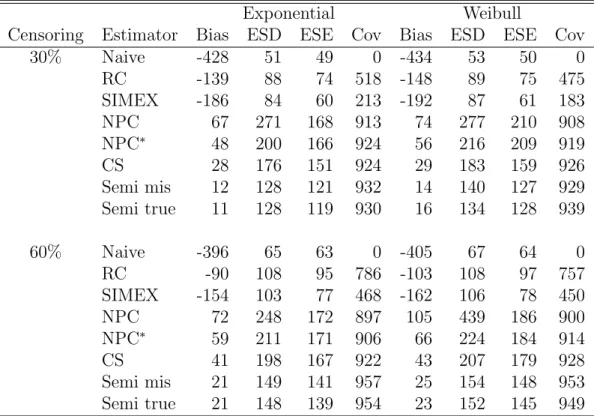
The results under independent censoring are summarized in Table 2.1, where we

(28)

and the coverage rate of a 95% confidence interval for various estimators of β. As we can see, the naive estimator is severely biased; both approximation methods, i.e. RC and SIMEX, are still considerably biased; the NPC and CS estimators are consistent estimators and yield smaller biases than the approximation methods. In all cases shown in the table, our proposed estimators yield the smallest biases among all and have much smaller standard deviations than other consistent estimators (i.e. the NPC and CS) which illustrates the efficiency of our methods. For example, our methods are 77% to 89% more efficient than the CS estimator. The NPC method occasionally yields strange solutions and these outliers inflate the empirical bias and standard deviation. To be

generous, we also report a cleaned version of NPC (labeled as NPC∗ in the table), where

we remove 0.5% to 2% of outliers in different cases. Such failure to converge has never occurred to our estimators and even after removing these outliers the NPC still has much larger standard deviations than ours. In addition, both the NPC and CS methods significantly underestimate the standard errors, and our further simulations reveal that this underestimation of standard error can be severe when either the measurement error is large or the censoring rate is high. In contrast, the estimated standard errors of our methods do not show obvious underestimation. One striking finding of particular interest

is that misspecification of p(x) in our methods does not cause obvious loss of efficiency.

The results under dependent censoring are reported in Table 2.2. These results tell

a rather similar story as Table 2.1. Our proposed method still vastly outperforms the

competing methods, which also suggests that the proposed estimator is robust to mild violation of the independent censoring assumption.

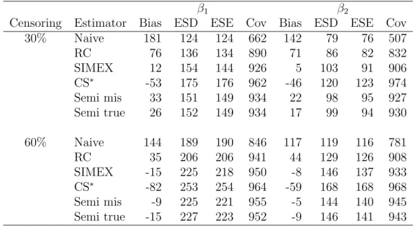
2.3.2 Simulation 2: a quadratic Cox regression model

To assess the performance of the proposed estimator when g(·) in (2.1) is nonlinear,

we considered the model λ(t | X) = λ0(t) exp(β1X +β2X2), where β1 = β2 = −1.

We generated X from Normal(−1,1) and W = X +U where U ∼ Normal(0, σ2

(29)

Table 2.1 Estimation results of β under Simulation 1 and independent censoring. The results are based on 1,000 replications.

Exponential Weibull

Censoring Estimator Bias ESD ESE Cov Bias ESD ESE Cov

30% Naive -428 51 49 0 -434 53 50 0 RC -139 88 74 518 -148 89 75 475 SIMEX -186 84 60 213 -192 87 61 183 NPC 67 271 168 913 74 277 210 908 NPC∗ 48 200 166 924 56 216 209 919 CS 28 176 151 924 29 183 159 926 Semi mis 12 128 121 932 14 140 127 929 Semi true 11 128 119 930 16 134 128 939 60% Naive -396 65 63 0 -405 67 64 0 RC -90 108 95 786 -103 108 97 757 SIMEX -154 103 77 468 -162 106 78 450 NPC 72 248 172 897 105 439 186 900 NPC∗ 59 211 171 906 66 224 184 914 CS 41 198 167 922 43 207 179 928 Semi mis 21 149 141 957 25 154 148 953 Semi true 21 148 139 954 23 152 145 949

Naive, the naive estimator; RC, regression calibration; SIMEX, the simulation ex-trapolation estimator; NPC, the nonparametric correction estimator of Huang and

Wang (2000); NPC∗, the NPC estimator after removing some outiers; CS, the

condi-tional score estimator; Semi mis and Semi true, the locally efficient semiparametric

estimators under the misspecified and true distribution of X, respectively; Bias, the

empirical bias (×103); ESD, the empirical standard deviation (×103); ESE, the mean

estimated standard error (×103_{); Cov, the empirical coverage probability of a 95%}

Wald confidence interval (×103_).

σU = 1/5. The rest of the simulation setting is similar to the setting described in

Simulation 1.

The NPC estimator was proposed for the case where g(·) is linear and therefore

was not included for comparison. Since no complete and sufficient statistic exists under this model, the CS approach cannot be applied directly. Instead, we considered the approximated conditional score method of Song, Davidian, and Tsiatis (2002), which is

based on a linear approximation using the delta method. The results forλ0(t) =t under

(30)

Table 2.2 Estimation results of β under Simulation 1 and dependent censoring. The results are based on 1,000 replications.

Exponential Weibull

30% Naive -432 52 50 0 -440 53 50 0 RC -143 88 75 492 -154 89 76 441 SIMEX -187 85 60 206 -195 87 61 190 NPC 72 264 166 918 88 287 178 907 NPC∗ 60 206 166 924 66 216 177 921 CS 35 178 153 938 36 190 163 937 Semi mis 6 130 119 934 8 137 128 927 Semi true 7 131 119 935 28 149 141 944 60% Naive -403 68 64 0 -419 69 66 0 RC -101 111 96 760 -126 112 99 696 SIMEX -159 107 78 470 -173 110 81 423 NPC 73 337 168 887 95 418 185 880 NPC∗ 53 216 167 896 61 231 183 893 CS 37 200 163 924 39 210 178 935 Semi mis 4 147 132 929 3 152 139 938 Semi true 3 149 134 924 -9 155 143 933

Note: The layout of the table is similar to Table 2.1.

biased. The proposed estimator is robust against misspecification ofp(x) and has smaller

bias than RC and approximated CS. The SIMEX estimator works surprisingly well under this particular setting and is comparable to our method.

2.4 Analysis of AIDS clinical trial data

We applied the proposed method to data from AIDS Clinical Trials Group (ACTG) 175 (Hammer et al., 1996) to assess the effects of antiretroviral therapies and baseline CD4 count on the time to AIDS or death in antiretroviral-naive patients. Four therapies were investigated in the ACTG 175 clinical trial, and previous studies (Hammer et al., 1996; Huang and Wang, 2000) found that the therapy using zidovudine alone is inferior to the other three therapies while the effects of the other three therapies are rather similar. Following Song and Huang (2005), we considered two treatment groups in our analysis,

(31)

Table 2.3 Results of the Simulation 2 based on 1,000 replications

β1 β2

30% Naive 181 124 124 662 142 79 76 507 RC 76 136 134 890 71 86 82 832 SIMEX 12 154 144 926 5 103 91 906 CS∗ -53 175 176 962 -46 120 123 974 Semi mis 33 151 149 934 22 98 95 927 Semi true 26 152 149 934 17 99 94 930 60% Naive 144 189 190 846 117 119 116 781 RC 35 206 206 941 44 129 126 908 SIMEX -15 225 218 950 -8 146 137 933 CS∗ -82 253 254 964 -59 168 168 968 Semi mis -9 225 221 955 -5 144 140 945 Semi true -15 227 223 952 -9 146 141 943

Note: The layout of the table is similar to Table 2.1. CS∗ is the approximated

conditional score estimator of Song, Davidian, and Tsiatis (2002).

zidovudine alone and the combination of the other three therapies. It is well known that CD4 measurements were subject to substantial measurement errors. Among the 1067 antiretroviral-naive patients in the study, 1036 had two CD4 measurements within 3 weeks of randomization and 31 had only one CD4 measurement. The censoring rate for the time to AIDS or death was 91%.

Following the literature, we used the log transformed CD4 count as a covariate in the proportional hazards model. It is well-known that the CD4 count measures were

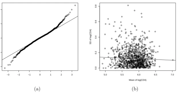
subject to a significant amount of measurement error. We used the graphical tools

described in Carroll et al. (2006) to check various assumptions on the measurement

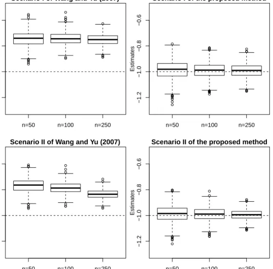
error. In the left panel of Figure 2.1, we show the normal Q-Q plot of the differences

between replicates of log(CD4) within the same subject. The plot indicates that the measurement error exhibits slightly heavy tails on both sides, which is a mild deviation

from the Gaussian assumption. In the right panel of Figure2.1, we also plot the standard

deviation of log(CD4) within a subject against the mean to check on the constant variance assumption. The regression line in this plot was fitted using the robust regression function

(32)

rlmin theMASSpackage inR. The estimated slope is -0.0184 with ap-value of 0.067, and therefore there is no clear violation of the assumption that the variance of measurement error is a constant. The estimated standard deviation is 0.182 for the measurement error and 0.276 for the true underlying log(CD4).

−3 −2 −1 0 1 2 3 −1.0 −0.5 0.0 0.5 1.0

QQ−Plot for the Differences

5.0 5.5 6.0 6.5 7.0 0.0 0.2 0.4 0.6 0.8

Constance Variance Plot

Mean of log(CD4)

SD of log(CD4)

(a) (b)

Figure 2.1 Model checking for the AIDS clinical trial data. (a) is the normal QQ plot

for the differences between replicates of log(CD4); (b) is the scatter plot of the standard deviation of log(CD4) within a subject versus the mean log(CD4) within the subject.

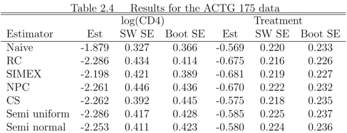
We considered a proportional hazards model with two covariates, the error-prone log(CD4) and an error-free treatment indicator which is zero for the zidovudine alone therapy and one for the other therapies. For the proposed locally efficient estimator, we considered two distributions for log(CD4), a normal distribution and a uniform

dis-tribution. In Table 2.4, we compare the estimation results based on various estimators

considered in the simulation studies. In addition to the parameter estimates, we provide two versions of standard errors estimated by either a sandwich formula or a bootstrap procedure with 1,000 bootstrap samples. As suggested by our simulation results, the sandwich formula can sometimes underestimate the true standard deviation, especially

(33)

for the NPC and CS estimators. The bootstrap standard error, even though is computa-tionally more expensive, is considered to be more reliable for a fair comparison among the different methods. Both the NPC and CS estimators are based on estimating equations, and the consistency of bootstrap for these estimators follows from the general theory by Chatterjee and Bose (2005) for bootstrapping estimating equations. Our estimator is based on a semiparametric estimating equation as we allow the number of splines and dimension of the estimating equation to diverge to infinity. We expect the consistency of bootstrap for our estimator to follow from similar arguments as in Chatterjee and Bose (2005), but a rigorous justification is out of the scope of this paper.

As we can see from Table 2.4, the treatment effect is not affected much by

measure-ment error in CD4, since the naive estimate of the treatmeasure-ment effect is rather similar to the CS and the proposed estimators. The RC, SIMEX and NPC methods, however, seem to have overdone with bias-correction for the treatment effect. The naive estimator for the coefficient of log(CD4), on the other hand, is significantly attenuated compared with other estimators. All methods that take into account the measurement error provide similar estimates for log(CD4) except for the SIMEX which still shows a small degree of attenuation. The proposed estimator under either Gaussian or uniform assumption for log(CD4) has a smaller bootstrap standard error than other consistent estimators (i.e. the CS and NPC), indicating some efficiency gain using our method.

2.5 Discussion

We propose a class of locally efficient semiparametric estimators for the proportional hazards models with covariates contaminated with measurement error. Compared with competing methods, the proposed estimator is robust against misspecification of the distribution of the true covariate and is semiparametrically efficient if this underlying distribution is correctly specified. We allow the effect of the error-prone variable on the

(34)

Table 2.4 Results for the ACTG 175 data

log(CD4) Treatment

Estimator Est SW SE Boot SE Est SW SE Boot SE

Naive -1.879 0.327 0.366 -0.569 0.220 0.233 RC -2.286 0.434 0.414 -0.675 0.216 0.226 SIMEX -2.198 0.421 0.389 -0.681 0.219 0.227 NPC -2.261 0.446 0.436 -0.670 0.222 0.232 CS -2.262 0.392 0.445 -0.575 0.218 0.235 Semi uniform -2.286 0.417 0.428 -0.585 0.225 0.237 Semi normal -2.253 0.411 0.423 -0.580 0.224 0.236

Note: Naive, the naive estimator; RC, the regression calibration method; SIMEX, the simulation extrapolation estimator; NPC, the nonparametric correction estimator of Huang and Wang (2000); CS, the conditional score estimator; Semi uniform and Semi normal, the proposed semiparametric estimators when log(CD4) is assumed to be uniformly and normally distributed, respectively; Est, estimate; SW SE, standard error estimated using a sandwich formula; Boot SE, the bootstrap standard error based on 1,000 bootstrap replications.

failure time to have a very general parametric form, under which a sufficient statistic for the true covariate usually does not exist. The likelihood function of the proportion hazards model involves the integral of the baseline hazard function, which makes a local estimating equation approach like the one proposed by Ma and Carroll (2006) difficult to implement. We circumvent this difficulty using spline approximations. Our numerical studies show that our method vastly outperforms competing methods.

The efficiency loss for the proposed estimators under misspecified p∗(xxx | z) is

un-known. However, the simulation results in this paper, as well as those in Tsiatis and Ma (2004) and Ma and Carroll (2006), show that the loss is virtually negligible even if the misspecification of p∗(xxx | z) is severe. In practice, it is still advisable to propose a

proper specification ofp(xxx|z) using some graphical tools. When the measurement error

is very large, a nonparametric estimate of p(xxx|z) using deconvolution methods can also

be employed (Delaigle, Hall, and Meister, 2008).

Our method is developed under the independent censoring assumption, but can be extended easily to situations where censoring time also depends on the covariates. In

(35)

those cases, another proportional hazards model can be used to characterize the relation-ship between the censoring time and the covariates, λi,C(t) =λC(t) exp{gC(Xi,Zi, θθθ1,C)},

where gC(·) is a known function of Xi and Zi with a parameter θθθ1,C. We can redefine

the parameter of interest to be a combination of θθθ1 and θθθ1,C. Then a semiparametric

estimator can be constructed similarly and the locally efficient property of the estimator still holds. Under this setting, we can estimate not only the relationship between the failure time and the covariates but also the censoring mechanism.

2.6 Acknowledgments

The research of Li and Xu was partially supported by the US National Science Foun-dation (DMS-1314118). The research of Song was partially supported by US National Science Foundation(DMS-1106816) and US National Institute of Health (R01ES017030).

2.7 Appendix: technical proofs

Appendix A: proof of theorem 1

We use the notation Oe_p(·) and e

op(·) to denote the element-wise Op(·) and op(·) rates

of a vector or a matrix. For any real valued matrix A, define its spectral norm as

kAk = maxkxxxk6=0kAxxxk/kxxkx and its Frobenius norm as kAkF = {tr(ATA)}1/2. Put In(θθθ) = E{Jn(θθθ)}=E{−∂/∂θθθS∗eff(O, θθθ)}.

We use C, C1 and C2 as generic notation for positive constants. To show the

exis-tence of consistent solutions, we only need to verify the following condition (Ortega and

Rheinboldt, 1970; Wang, 2011): for any >0, there exists a constant ∆>0 such that,

for sufficiently large n,

pr{ sup kθθθn−θθθ∗k=∆δn (θθθn−θθθ ∗ )T Sn(θθθn)<0} ≥1−. (2.11)

(36)

For any ΘΘΘk= (θθθ1,k, νk, νC,k) with νk(t) =BeT₁(t)γγγ_k and νC_,k(t) =BeT₂γγγ_C_,k, k = 1,2, denote θθθk= (θθθ T 1,k, γγγ T k, γγγ T C,k)

T_{. By Lemma 6.1 of Zhou} _{et al. (1998),}

0< C1 ≤ kνkk2/kγγγkk 2 ,kνC,kk2/kγγγC,kk 2 _≤ C2 <∞, and hence 0< C1 ≤ kΘΘΘkk2/kθθθkk2 ≤C2 <∞, k = 1,2.

By the definition in (2.10), it is easy to see along the direction ΘΘΘ†

S∗(ΘΘΘ1; ΘΘΘ2) =θθθT2S

∗

eff(θθθ1).

For anyθθθ such that kθθθ−θθθ∗k ≤Cδn, following similar lines of proof for equation (12) in

Tsiatis and Ma (2004) while taking into account the asymptotic bias in S∗_eff(θθθ), we get

In(θθθ) =E{S∗eff(θθθ)S T eff(θθθ)}+Oe(δ_n). (2.12) By assumption (1), if kΘΘΘ1−ΘΘΘ0k ≤Cδn 0< C1 ≤ θθθT 2In(θθθ1)θθθ2 kθθθ2k2 E{S ∗_(Θ_Θ_Θ 1; ΘΘΘ2)S(ΘΘΘ1; ΘΘΘ2)} kΘΘΘ2k2 +O(K ×δn)≤C2 <∞, (2.13)

where, for any sequences of positive constants {an} and {bn}, an bn means an/bn is

bounded away from both 0 and ∞. It is easy to see that |Jn(θθθ)−In(θθθ)| = Oe(n−1/2)

and hence kJn(θθθ) − In(θθθ)kF = O(Kn−1/2). Therefore, as n → ∞, with probability

approaching 1 0< C1 ≤ θθθT 2Jn(θθθ1)θθθ2 kθθθ2k2 ≤C2 <∞ (2.14)

for anyθθθ2 provided that kθθθ1 −θθθ

∗

k ≤Cδn.

Finally, we verify (2.11). For anyθθθn satisfying kθθθn−θθθ

∗

k= ∆δn, (θθθn−θθθ

∗ )T

Sn(θθθn) :=

An1+An2 with An1 = (θθθn−θθθ∗)TSn(θθθ∗) and An2 =−(θθθn−θθθ∗)TJn(¯θθθn)(θθθn−θθθ∗) where ¯θθθn

is betweenθθθ∗ andθθθn. It is easy to see

E(|An1|)≤ kθθθn−θθθ ∗ kE{kSn(θθθ ∗ )k} ≤C∆δ_n2, An2 ≤ −C1kθθθn−θθθ∗k2 ≤ −C1∆2δn2.

(37)

We can choose ∆ large enough to make the probability of {(θθθn −θθθ

∗ )T_S

n(θθθn) < 0}

approaching 1.

Appendix B: proof of theorem 2

By Taylor’s expansion

0 =Sn(bθθθ_n) =S_n(θθθ∗)−J_n(θθθ∗)(bθθθ_n−θθθ∗) +Oep(kθθθb_n−θθθ∗k2).

By Theorem1 and assumption (2), it is easy to verifykbθθθn−θθθ∗k2 =op(n−1/2). Equation

(2.14) also guarantees thatJn is non-singular and its eigenvalues are bounded away from

0. It follows that b θθθn−θθθ ∗ =J−_n1(θθθ∗)Sn(θθθ ∗ ) +_eop(n−1/2). (2.15)

Rewrite Sn and S∗eff as Sn = (ST1n,S

T 2n) T and S∗_eff = (S∗T 1eff,S∗ T 2eff) T , according to the partitionθθθ = (θθθT 1, θθθ T 2) T_{. Write}_J

n and its inverse J−n1 as

Jn =    J11n J12n J21n J22n    , J −1 n =    J11 n J12n J21 n J22n   .

The first p equations in (2.15) becomes

b θθθ1n−θθθ10 =J11n(θθθ ∗ )S1n(θθθ∗) +J12n (θθθ ∗ )S2n(θθθ∗) +eop(n −1/2 ), (2.16) where J11 n = (J11n−J12nJ−221nJ21n)−1 and J12n = (J11n−J12nJ−221nJ21n)−1J12nJ−221n.

Define the partition ofIn(θθθ) similarly asJn(θθθ), put ΓΓΓn(θθθ∗) = (I11n−I12nI−221nI21n)|θθθ=θθθ∗,

ΣΣΣn(θθθ ∗ ) = cov(S∗_1eff +I12nI−221nS ∗ 2eff)|θθθ=θθθ∗ and Γ Γ Γ = lim n→∞ΓΓΓn, ΣΣ = limΣ n→∞ΣΣΣn. (2.17)

It follows from (2.16) and (2.17) that

n1/2(θθθb₁_n−θθθ₁₀) = n1/2J11_n(θθθ∗){S₁_n(θθθ∗) +J₁₂_n(θθθ∗)J−₂₂1_n(θθθ∗)S₂_n(θθθ∗)}+ e op(1) = n1/2ΓΓΓ−1{S1n(θθθ ∗ ) +I12n(θθθ ∗ )I−₂₂1_n(θθθ∗)S2n(θθθ ∗ )} +R1+R2+oep(1), (2.18)

(38)

where R1 = n1/2J11n(θθθ ∗ ){J12n(θθθ∗)J−221n(θθθ ∗ )−I12n(θθθ∗)I−221n(θθθ ∗ )}S2n(θθθ∗), R2 = n1/2{J11n (θθθ ∗ )−ΓΓΓ−1}{S1n(θθθ ∗ ) +I12n(θθθ ∗ )I−₂₂1_n(θθθ∗)S2n(θθθ ∗ )}.

We first calculate the rate of R1. It is easy to see kJ11nkF = Op(1) and J12nJ−221n−

I12nI−221n= (J12n−I12n)J−221n+I12n(J−221n−I

−1

22n). By straightforward calculations,k(J12n−

I12n)J−221nkF ≤ kJ12n−I12nkFkJ22−1nk = Op{(K/n)1/2} ×Op(1) = op(1). For the second

term,kI12nkF =O(K1/2) and kJ−221n−I

−1

22nkF =kI

−1

22n(J22n−I22n)I22−1nkF× {1 +op(1)}(see

Section 5.8 in Horn and Johnson (1985)). Equation (2.13) implies kI−₂₂1_nk = O(1), and

hencekI−₂₂1_n(J22n−I22n)I−221nkF=Op(kJ22n−I22nkF). Entries ofJ22nare partial derivatives

with respect to spline coefficients. Because B-splines have compact supports, J22n has a

band matrix structure. In other word, there are only a fixed number of non-zero entries in each row of J22n. Detailed calculations show kJ22n−I22nk2F = Op(K/n). Therefore, kJ12nJ−221n−I12nI−221nkF=Op(Kn−1/2). By (2.9),kS2n(θθθ ∗ )k2 _{≤ k}_S 2n(θθθ ∗ )−E{S2n(θθθ ∗ )}k2₊ kE{Sn2(θθθ ∗ )}k2 ₌_O p(K/n+Kmax i=1,2K −2ri

i ).Under assumption (2), the results above lead

to

kR1k=Op(K3/2n−1/2 +K3/2max i=1,2K

−ri

i ) = op(1).

By similar calculations as above, we have k(J11n−J12nJ−221nJ21n)−ΓΓΓnkF ≤ kJ11n−

I11nkF+k(J12n−I12n)J22−1nJ21nkF+kI12n(J−221nJ21n−I−221nI21n)kF =Op(n−1/2)+Op(Kn−1/2)+ Op(K3/2n−1/2) =op(1). Since ΓΓΓ−n1 →ΓΓΓ −1 , kJ11 n (θθθ ∗ )−ΓΓΓ−1kF =op(1) and kR2k=op(n1/2kS1n(θθθ ∗ ) +I12n(θθθ ∗ )I−₂₂1_n(θθθ∗)S2n(θθθ ∗ )k) = op(1).

Since R1 and R2 are higher order terms, (2.18) can be re-written as

n1/2(bθθθ₁_n−θθθ₁₀) = n−1/2 n X i=1 Γ ΓΓ−1 S∗_1eff(Oi, θθθ∗) +I12n(θθθ∗)I−221n(θθθ ∗ )S∗_2eff(Oi, θθθ∗) +op(1). (2.19) It is easy to see nvar(bθθθ₁_n−θθθ₁₀) = ΓΓΓ−1ΣΣΣ_nΓΓΓ−1 +o(1) → ΓΓΓ−1ΣΣΣΓΓΓ−1, and the asymptotic

(39)

When p(xxx|z) is correctly specified, similar to (2.12), we can show that In(θθθ ∗ ) =E{Seff(O, θθθ ∗ )ST eff(O, θθθ ∗ )}+Oe(δ_n).

Then it is easy to verify ΣΣΣ = ΓΓΓ.

Appendix C: proof of theorem 3

We only need to show bθθθ₁_n is semiparametrically efficient when p(xxx | z) is correctly

specified. By (2.19),bθθθ₁_n is asymptotically linear with the influence function

ϕϕϕ(O) = ΓΓΓ−1S1eff(O, θθθ ∗ ) +I12n(θθθ ∗ )I−₂₂1_n(θθθ∗)S2eff(O, θθθ ∗ ) .

By our construction of the efficiency scores, Seff ⊥ (Λ1+ Λ2) and hence ϕϕϕ⊥ (Λ1+ Λ2).

Therefore, to show semiparametric efficiency, it suffices to proveϕϕϕ⊥(Λ3+ Λ4).

For any K-dimensional constant vector v, (2.12) implies

hϕϕϕ,ST

2effvi= ΓΓΓ

−1_{E

(S1effST2effv)−E(I12nI22−1nS2effST2effv)}=O(max

i=1,2K

−ri

i ). (2.20)

Recall S2eff(O) = Sθθθ2(O)−Π{Sθθθ2(O)|Λ1+ Λ2}, where Sθθθ2(O) = {S T γγγ1(O),S T γγγ2(O)} T_, Sγγγ1(O) = E{Sγγγ1(V,∆,X,Z)|O}=E{∫Be1(u) dM(u,X,Z)|O}, Sγγγ2(O) = E{Sγγγ2(V,∆,X,Z)|O}=∫Be2(u) dMC(u).

An arbitrary element h(O) in Λ3+ Λ4 can be expressed as

h(O) = c1E{∫ a1(u) dM(u,X,Z)|O}+c2∫ a2(u) dMC(u)

for some integrable functions a1(·), a2(·) and constants c1 and c2. Because the H¨older

class defined in (2.8) is dense inL2 _{functional space, there exists a}_K

i-dimensional vector

vi such thatkai(u)−Be_iT(u)v_ik=O(K_i−ri), i= 1,2. Let v= (c₁v₁T, c₂v₂T)T, then h(O) = c1E{∫ BeT₁(u)v₁ dM(u,X,Z)|O}+c₂∫BeT₂(u)v₂ dM_C(u) +O(max i=1,2K −ri i ) = vT Sθθθ2(O) +O(max i=1,2K −ri i ) = vT S2eff(O) +vTΠ{Sθθθ2(O)|Λ1+ Λ2}+O(max i=1,2K −ri i ). (2.21)

(40)

Equations (2.20) and (2.21) imply hϕϕϕ(O), h(O)i = O(max i=1,2K −ri i ) = o n −1/2 for any

h(O) ∈Λ3 + Λ4. Consequently, ϕϕϕ(O) is an efficient influence function which completes

the proof.

Appendix D: Recursive formula for B-splines

Let a < κ1 < κ2 <· · ·< κJ < b be the sequence of inner knots as defined in Section 2.2.3 and let κ1−r = . . . = κ0 = a and κJ+1 = . . . = κJ+r = b be the boundary knots.

To distinguish B-splines with different orders, denote {Bj,k(t);j = 1, . . . , J +k} as the

collection of kth order B-splines defined on the same set of inner knots for k = 1, . . . , r. The first order B-splines or the constant B-splines are defined as

Bj,1(t) = 1 fort ∈[κj−1, κj), 0 otherwise, j = 1, . . . , J + 1.

Then the kth order B-splines can be evaluated using the following recursive formula

Bj,k(t) = t−κj−k κj−1−κj−k Bj−1,k−1(t) + κj −t κj−κj−k+1 Bj,k−1(t), j = 1, . . . , J+k,