A Probabilistic Model for Dirty Multi-task Feature Selection
Daniel Hern´andez-Lobato [email protected]
Universidad Aut´onoma de Madrid, Computer Science Department, Madrid, 28049, Spain
Jos´e Miguel Hern´andez-Lobato [email protected]
Harvard University, School of Engineering and Applied Sciences, Cambridge, MA 02138, USA
Zoubin Ghahramani [email protected]
University of Cambridge, Department of Engineering, Cambridge CB2 1PZ, UK
Abstract
Multi-task feature selection methods often make the hypothesis that learning tasks share relevant and irrelevant features. However, this hypothe-sis may be too restrictive in practice. For exam-ple, there may be a few tasks with specific rele-vant and irrelerele-vant features (outlier tasks). Sim-ilarly, a few of the features may be relevant for only some of the tasks (outlier features). To ac-count for this, we propose a model for multi-task feature selection based on a robust prior distri-bution that introduces a set of binary latent vari-ables to identify outlier tasks and outlier features. Expectation propagation can be used for efficient approximate inference under the proposed prior. Several experiments show that a model based on the new robust prior provides better predictive performance than other benchmark methods.
1. Introduction
When the number of samples is smaller or equal to the number of attributes or features, regression problems are under-determined. In this case, a linear model is too com-plex to explain the observed data since an infinite number of model coefficients perfectly fit the data. In this context, sparsity,i.e., the assumption of zeros in the model coeffi-cients, plays a strong regularization role that can be use-ful to obtain estimates with good generalization properties. Sparsity can be favored by using sparsity enforcing priors in probabilistic models or by optimizing a loss function pe-nalized by a sparsity inducing norm (Carvalho et al.,2009; Jalali et al.,2010;Vogt & Roth,2010). The assumption of
Proceedings of the32nd International Conference on Machine
Learning, Lille, France, 2015. JMLR: W&CP volume 37.
Copy-right 2015 by the author(s).
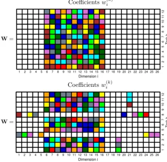
zeros in the model coefficients is equivalent to the assump-tion of only a few of relevant features for predicassump-tion. Multi-task feature selection methods are used to improve the process of inferring the model coefficients from the ob-served data under the sparsity assumption (Vogt & Roth, 2010; Hern´andez-Lobato et al., 2010; Obozinski et al., 2009; Xiong et al., 2007; Zhang et al., 2008). In these methods several tasks that have a common feature space are solved simultaneously, often under the assumption that the tasks share relevant and irrelevant features, as illustrated by Figure2(top). However, in some situations this hypothesis may be too restrictive (Jalali et al.,2010). As illustrated by Figure2(bottom), a few of the tasks may have specific rel-evant / irrelrel-evant features (outlier tasks), and a few of the features may be arbitrarily relevant / irrelevant across tasks (outlier features). In this situation, traditional multi-task feature selection methods are expected to perform poorly. In this paper we propose a multi-task feature selection model, based on a robust prior distribution, that is expected to have better properties in the presence of diverse tasks, i.e., data with the properties described above. Exact infer-ence is intractable in such a model. However, expectation propagation can be used for efficient approximate inference (Minka,2001). Several experiments involving the recon-struction of gene regulatory networks, the denoising of nat-ural images and the prediction of drug sensitivity from mi-croarray data illustrate the benefits of the model proposed. Specifically, it has better prediction properties than other methods from the literature and it can be used to success-fully identify relevant attributes for prediction, alongside with outlier tasks and features, which may be useful to bet-ter understand the characbet-teristics of the observed data.
2. Dirty Multi-task Feature Selection
Assume K regression tasks with data {X(k),y(k)}K k=1,
of targets for taskk, respectively. All tasks share the same dattributes or features, but feature values can be different across tasks. A linear model is considered for each task, i.e.,y(k)=X(k)w(k)+(k), wherew(k)∈
Rdis the vec-tor of model coefficients for taskkand(k)∼ N(0,Iσ2
(k))
is Gaussian noise with varianceσ2
(k). LetWbe aK×d
matrix whosek-th row isw(k)andYa matrix whosek-th
row isy(k). DefineX ={X(k)}K
k=1andσ2={σ2(k)}
K k=1.
The likelihood forWandσ2is:
p(Y|X,W,σ2) =
K
Y
k=1
N(y(k)|X(k)w(k),Iσ(2k)). (1)
Moreover, feature selection for each task, or equivalently, sparsity in eachw(k)is expected to be beneficial. We also
assume that theKtasks share relevant and irrelevant fea-tures, but we allow for smalldeviationsfrom this hypothe-sis. All this prior knowledge is introduced in the model by a robust prior forWdescribed in the next section. 2.1. Robust prior distribution
The prior considered is based on the discrete mixture prior introduced in (Carvalho et al.,2009). Thus, we first de-scribe and motivate the use of that prior to favor sparse so-lutions. Then, we show how it can be extended to perform feature selection across several tasks in a robust way. 2.1.1. DISCRETE MIXTURE PRIOR
This is aspike and slabprior in which thei-th coefficient of taskksatisfiesw(ik)∼(1−ρ)δ0+ρπ(w
(k)
i ), whereρis the prior inclusion probability,δ0is a point of probability
mass at zero, andπ(·)is a density that specifies the distri-bution of the coefficients that are not zero. Eachw(ik)isa priorizero with probability (1−ρ). In (Carvalho et al., 2009) it is suggested forπ(·)the Strawderman-Berger dis-tribution (Strawderman, 1971; Berger, 1980), which has Cauchy-like tails and yet allows for a closed form convolu-tion with a Gaussian likelihood. This distribuconvolu-tion is a scale mixture of Gaussians (Armagan et al.,2011) defined as:
πwi(k)= Z N(wi(k)|0, λ2i) λi (λ2 i + 1) 3 2 dλi = √1 2π 1− |w (k) i | Φ(−|wi(k)|) N(w(ik)|0,1) ! , (2)
where| · |denotes absolute value,Φ(·)is the cdf of a stan-dard Gaussian distribution,N(·|0,1)is the standard Gaus-sian density, andλi/(λ2i + 1)
3
2 is the density assumed for λi. Figure1(left and middle) compares the discrete mix-ture prior with other priors from the literamix-ture (an arrow means a point of probability mass). We observe that the discrete mixture has heavy tails to explain coefficients that
significantly differ from zero. It also has a point mass at zero that allows for exact zeros in the coefficients.
Letσ2
(k) = 1andX
(k) =I, and defineκi = 1/(1 +λ2
i). Carvalho et al. (2009) shows that the posterior mean for w(ik) is in this case(1 −κi)y
(k)
i , where κi is a random shrinkage coefficient. Figure 1 (right) displays the prior density forκi that results from each prior for w(ik). The prior forκiis obtained by applying the change of variables κi= 1/(1 +λ2i)to the prior forλi, which in the case of the discrete-mixture prior is a mixture between the distribution for λi assumed in (2) and a point mass at zero. Figure1 (right) shows that under the discrete-mixture priora priori we expect to observeκi = 1as a consequence of the point mass at one in the prior forκi. Furthermore, we also expect to observeκi ≈0as a consequence of the density tending to infinity at zero. These two values forκi correspond re-spectively to total shrinkage (zero values) and no shrinkage at all (non-zero values) for w(ik). By contrast, under the other priors forwi(k)the density forκitends to zero at zero (Laplace) or tends to zero at one (Student’s T). This means that these priors will shrink relevant coefficients and will not shrink irrelevant coefficients, respectively. Thus, the discrete mixture prior can be considered as agolden stan-dardfor learning under sparsity (Carvalho et al.,2009). 2.1.2. EXTENSION OF THE DISCRETE-MIXTURE PRIOR The previous prior is extended to perform feature selection across several tasks. We assume that the tasks share in gen-eral relevant and irrelevant features, but we consider a few outlier tasks with specific relevant / irrelevant features and a few outlier features that may be arbitrarily relevant / irrel-evant for each task. This is illustrated in Figure2(bottom). Tasks4and8are outlier tasks and features19and21are outlier features. All other tasks and features share the hy-pothesis of jointly relevant / irrelevant features across tasks. To model this type of prior knowledge we introduce the following binary latent variables:
zi Indicates whether featurei is an outlier (zi = 1) or not
(zi= 0). If it is an outlier it can be independently relevant
or irrelevant for each task.
ωk Indicates whether task k is an outlier (ωk = 1) or not
(ωk = 0). If it is an outlier it can have specific relevant
and irrelevant features for prediction.
γi Indicates whether the non-outlier featureiis relevant (γi=
1) for prediction or not (γi = 0) in all tasks that are not
outliers,i.e., those tasks for whichωk= 0.
τi(k) Indicates whether, given that taskkis an outlier task,i.e.,
ωk = 1, featureifor that task is relevant (τi(k) = 1) or
irrelevant (τi(k)= 0) for prediction.
−3 −2 −1 0 1 2 3 0.0 0.1 0.2 0.3 0.4 0.5 0.6 0.7 Probability Dens ity Discrete Mixture Gaussian Student−t(df=1) Laplace 4 5 6 7 0.000 0.005 0.0 10 0.015 0.020 0.025 Probability Dens ity Discrete Mixture Gaussian Student−t(df=1) Laplace 0.0 0.2 0.4 0.6 0.8 1.0 0 1 2 3 4 5 Probability Density Discrete Mixture Student−t(df=1) Laplace
Figure 1.(left) Density of different priors. Note the spike of the discrete mixture at the origin. (middle) Tails of the different priors. (right) Prior density of the shrinkage parameterκifor the discrete mixture prior and for other priors from the literature.
1 2 3 4 5 6 7 8 9 10 11 12 13 14 15 16 17 18 19 20 21 22 23 24 25 26 1 2 3 4 5 6 7 8 9 10 11 12 Dimension i Task k 1 2 3 4 5 6 7 8 9 10 11 12 13 14 15 16 17 18 19 20 21 22 23 24 25 26 1 2 3 4 5 6 7 8 9 10 11 12 Dimension i Task k
Figure 2.(top) Traditional multi-task feature selection: All tasks share relevant and irrelevant features (model coefficients). (bot-tom) Dirty multi-task feature selection: Most tasks share relevant and irrelevant features, but we allow for outlier tasks (tasks4and
8) and for outlier features (dimensions19and21). White squares represent irrelevant coefficients that are equal to zero. Colored squares represent relevant coefficients with non-zero values.
that particular feature is relevant for prediction in task k
(ηi(k)= 1) or not (ηi(k)= 0).
Let Ω be the collection of all these latent variables, i.e.
Ω = {z,ω,γ,{τ(k)}K k=1,{η
(k)}K
k=1}. Given the latent
variables we can specify the prior distribution forW:
p(W|Ω) = d Y i=1 K Y k=1 p(wi(k)|Ω), (3) wherep(wi(k)|Ω) = {π(w(ik))ηi(k)δ1−η (k) i 0 } zi{[π(w(k) i ) τi(k) δ1−τ (k) i 0 ]ωk[π(w (k) i )γiδ 1−γi
0 ]1−ωk}1−zi. Under this prior a
coefficientwi(k)is different from zero if (i) it corresponds
to an outlier feature (zi= 1) relevant for taskk(ηi(k)= 1); or (ii) it does not correspond to an outlier feature (zi = 0), but it corresponds to an outlier task (ωk = 1) and the feature is relevant for that task (τi(k) = 1); or (iii) it does not correspond to an outlier feature (zi= 0), nor an outlier task (ωk = 0), but the feature is relevant for prediction across tasks(γi = 1). Otherwise, the coefficient is zero. The hyper-priors for the latent variables are Bernoullis with parametersρz, ρω,ργ,ρτ andρη,i.e., we setp(z|ρz) =
Qd i=1Bern(zi|ρz), p(ω|ρω) = QK k=1Bern(ωk|ρω), p(γ|ργ) = Qd i=1Bern(γk|ργ), p({τ (k)}K k=1|ρτ) = QK k=1 Qd i=1Bern(τ (k) i |ρτ)and finallyp({η(k)}Kk=1|ρη) = QK k=1 Qd i=1Bern(η (k)
i |ρη). The hyper-prior for each ρz, ρω,ργ,ρτandρηis a beta distribution with parametersa0
andb0, e.g.,p(ρz) = Beta(ρz|a0, b0) for the case ofρz.
Furthermore, we seta0 = 1andb0 = 1which leads to a
uniform distribution so that no particular hyper-parameter value is favored a priori. These uniform priors allow to identify each hyper-parameter value from the training data. Last, we set the hyper-prior for the noise of each task to be an inverse gamma distribution, i.e., p(σ2) =
QK
k=1InvGam(σ 2
(k)|α0, β0), where we specifyα0= 5and
β0= 5. These parameter values are equivalent to the prior
observation in each task of 10 data instances with noise variance equal to1. Furthermore, they also produce high variance in the prior distribution which allows for the iden-tification of the correct level of noise of each task using the training data only. An alternative formulation of the prior that assumes the same level of noise for each task is also considered. Namely, we setp(σ2) =InvGam(σ2|α0, β0),
where each entry inσ2is constrained to be equal toσ2.
2.2. Prediction and identification of relevant features Defineρ = {ρz, ρω, ργ, ρτ, ρη}. The joint probability of the targetsYand the latent variablesW,Ω,ρandσ2is:
p(Y,W,Ω,ρ,σ2|X) =p(Y|X,W,σ2)p(W|Ω)×
where p(Y|X,W,σ2) is given by (1), p(W|Ω) is
given by (3), p(Ω|ρ) = p(z|ρz)p(ω|ρω)p(γ|ργ)
p({τ(k)}K
k=1|ρτ)p({η(k)}kK=1|ρη) and p(ρ) = p(ρz)
p(ρω)p(ργ)p(ρτ)p(ρη). This joint distribution is normal-ized with respect toW,Ω,ρandσ2to get a posterior:
p(W,Ω,ρ,σ2|Y,X) = p(Y,W,Ω,ρ,σ
2|X)
p(Y|X) . (5)
The posterior is used to compute predictions for the target value ynew of a new un-observed
in-stance xnew of task k. Namely, p(ynew|xnew) = P Ω R N(ynew|xTneww (k), σ2 (k))p(W,Ω,ρ,σ 2|Y,X)dW
dρdσ2. The probability that a particular w(k)
i is differ-ent from zero can be computed similarly. For this, we eliminate variables in (5) and sum the posterior probabil-ities of the three events described in Section 2.1.2, i.e.,
p(wi(k) 6= 0|Y,X) = p({zi = 1 ∩ ηi(k) = 1} ∪ {zi =
0 ∩ ωk = 1 ∩ τ
(k)
i = 1} ∪ {zi = 0 ∩ ωk = 0 ∩ γi =
1}|Y,X). Finally, the probability that taskkis an outlier, p(ωk = 1|Y,X), or the probability that feature i is an outlier,p(zi= 1|Y,X), are computed in a similar way. The computation of all the expressions described in this section, except (4), is intractable for typical problems. Thus, we have to resort to approximate inference methods.
3. Expectation propagation (EP)
EP is an efficient mechanism for approximate inference (Minka, 2001). EP approximates each factor in (4) that is not inside a particular exponential familyF of distribu-tions with an un-normalized factor that is inside F. We setF to be the product of Gaussian distributions onW, Bernoulli distributions onΩ, beta distributions onρand in-verse gamma distributions onσ2.Fis closed under
prod-uct and division operations. The only factors in (4) that are not inF are those of the likelihood (1),p(W|Ω)and p(Ω|ρ). The hyper-prior forρis beta, and the hyper-prior forσ2is inverse gamma so they need not be approximated.
In EP each likelihood factor corresponding to the n-th instance of the k-th task (x(nk), y
(k) n ) is ap-proximated as p(yn(k)|w(k),xn(k), σ2(k)) = N(y(nk)| (x(nk))Tw(k), σ(2k)) ≈ f˜ (k) n (w(k), σ2(k)) = ˜c (k) n N((x(nk))Tw(k)|m˜(nk),˜vn(k))InvGam(σ2(k)|˜an(k),˜b(nk)). The approximation of each factor p(w(ik)|Ω)
that appears in p(W|Ω) in (3) is p(w(ik)|Ω) ≈
˜
gi(k)(wi, zi, ωk, γi, τi(k), ηi(k)) = ˜si(k)N(wi|m˜i(k),σ˜2(i,k))
Bern(zi|p˜z(i,k))Bern(ωk|p˜
(i,k) ω )Bern(γi|p˜ (i,k) γ )Bern(τ (k) i
|p˜(τi,k))Bern(ηi(k)|p˜(ηi,k)). Finally, each factor in p(Ω|ρ) is approximated following a similar princi-ple. For example, for p(zi|ρz) the approximation is
Bern(zi|ρz) ≈ h˜(zi)(zi, ρz) = ˜κ (i) z Bern(zi|p˜ (i) z )Beta(ρz| ˜ a(zi),˜b (i)
z ). The approximation of the other factors in p(Ω|ρ)is equivalent to this one. All the parameters with the superscript˜are adjusted by EP, as described below. The EP approximation of the joint distribution (4) replaces each exact factor by the corresponding approximate one. Denote byq˜this approximation. After normalization, the joint distribution (4) becomes the exact posterior (5). Sim-ilarly, after normalizationq˜becomes the EP posterior ap-proximationq:
q(W,Ω,ρ,σ2) =q˜(W,Ω,ρ,σ
2)
Zq , (6)
which is inside ofFbecauseFis closed under the product operation. The parameters ofqare obtained from the prod-uct of all the factors inq˜andZq can be readily computed because q˜is an un-normalized parametric distribution in-side ofF. Givenq, all the expressions in Section2.2can be approximated by replacing the exact posterior withq. EP refines until convergence each approximate factor f˜. For this,qold ∝q/f˜is computed.qoldhas the same form as qbecauseq,f˜∈ F. Then, an updated posterior approxima-tion qnew is obtained by minimizing the Kullback-Leibler divergence betweenf qoldandqnew, KL(f qold||qnew), where
f denotes the exact factor associated to f˜. The updated approximate factor is f˜ = Zfqnew/qold, whereZf is the normalization constant of f qold. This guarantees that f˜
is similar to the exact factor in regions of high posterior probability, as estimated by qold. The minimization of
KL(f qold||qnew)with respect toqnewhas a global optimum
found by matching expected sufficient statistics between f qold andqnew (Bishop,2006). These expectations can be
obtained from the derivatives oflogZf with respect to the (natural) parameters ofqold, as indicated bySeeger(2006). A contribution of this paper is the computation ofZf for the factors in p(W|Ω). In that case,Zf is a probabilis-tic mixture of the convolution of the Strawderman-Berger prior π(·)with a Gaussian distribution, i.e., the posterior distribution for w(ik) under qold, and the convolution of
the point probability mass at the origin,δ0, with the same
Gaussian. Fortunately, the Strawderman-Berger prior has a closed form convolution with the Gaussian distribution. Johnstone & Silverman (2005) provide the analytic solu-tion when the variance of the Gaussian is one. We provide the solution when this is not the case. The complete details about EP are found in the supplementary material, along-side with an R implementation of the proposed method. Whend > Nk, whereNkis the number of instances of task kanddis the number of features, the covariance matrix of the likelihood of each task in (1) is low rank. EP is able to exploit this and it has a cost that scales likeO(PK
k=1N 2
4. Related work
There are several works in the literature focusing on feature selection within a multi-task learning setting. In this sec-tion they are described. For example, Hern´andez-Lobato et al.(2010) propose a model based on thespike-and-slab prior (Mitchell & Beauchamp,1988) to determine whether a feature is either relevant or irrelevant across all tasks. The spike-and-slabprior is also used in (Jebara,2004), where a multi-task feature selection method is derived using the maximum entropy discrimination formalism. In (Obozin-ski et al.,2009;Vogt & Roth,2010) the group LASSO is considered as an efficient estimator that selects common features across tasks by penalizing a mixed norm of the model coefficients. The work presented byArgyriou et al. (2007) is based on a similar approach. Finally, in (Xiong et al.,2007) a set of common relevant features across tasks is found using the automatic relevance determination prin-ciple. In summary, all these works assume jointly relevant and irrelevant features across tasks, ase.g.in Figure2(top), and are hence expected to perform poorly when this hy-pothesis is not fully satisfied, ase.g.in Figure2(bottom). There are other methods that have been proposed to re-lax the hypothesis of jointly relevant and irrelevant features across all tasks. In (Jalali et al.,2010) a dirty model consid-ers a mixed norm to penalize the model coefficients of sev-eral tasks. Specifically,W=P+QwherePis penalized with the`1norm andQwith the the`1,∞norm. A simi-lar model can be derived using the`1,2norm instead (Vogt
& Roth,2010). The estimator employed selects a common subset of relevant features for all the tasks, but it allows for tasks with additional specific relevant features. The result is a generalization of the group LASSO (Obozinski et al., 2009;Vogt & Roth,2010), which is expected to be more robust to outlier tasks in the learning process, but not to be as flexible as the model proposed in this paper. Another method introduced for this purpose is found in (Gong et al., 2012). This robust multi-task feature learning model also definesW=P+Qand estimates the model coefficients
Wby penalizing bothPandQT with the`
1,2norm. The
intuition behind this idea is that if thek-th row ofQis not zero after the estimation, taskkis an outlier task with all features relevant for prediction. However, again this a less flexible assumption than the one we make. In particular, the two works just described assume that all tasks share a few relevant features, although they allow for some arbi-trary tasks to have extra relevant features. This means that they cannot model outlier tasks, (e.g., tasks 4 and 8 in Fig-ure2(bottom)), unlike the approach proposed in this work. Hern´andez-Lobato & Hern´andez-Lobato (2013) consider that tasks do not share common relevant and irrelevant tures for prediction, but common dependencies in the fea-ture selection process. These dependencies are induced
from the data using a generalization of the horseshoe prior for feature selection (Carvalho et al.,2009). The princi-ple they follow is hence more flexible than the assumption made by the models described in the first paragraph of this section. However, such an approach is expected to be sub-optimal when most tasks actually share relevant and irrel-evant features for prediction, which is the hypothesis we assume and the one that is displayed in Figure2(bottom). Finally, some works in the literature also consider modeling outlier tasks in multi-task learning,e.g., (Xue et al.,2007; Passos et al.,2012). However, they do not consider sparsity in the model coefficients and are hence expected to perform poorly when this hypothesis is actually satisfied in practice.
5. Experiments
We compare the proposed model for dirty multi-task fea-ture selection (DMFS) with single task learning (STL) and with a model for multi-task feature selection (MFS) that assumes relevant and irrelevant features shared across all tasks. STL and MFS are particular cases of DMFS with all tasks being outliers (STL) and with no outlier tasks nor out-lier features (MFS). We also compare results with the meth-ods described in Section4. That is, the dirty model (DM) of Jalali et al.(2010), the robust multi-task feature learn-ing method (RMFL) ofGong et al.(2012) and the model for learning feature selection dependencies (MFSDep) of
Hern´andez-Lobato & Hern´andez-Lobato (2013). In DM and RMFL we choose hyper-parameters using a grid search guided by an inner cross-validation method. In MFSDepwe
use type-II maximum likelihood for this (Bishop, 2006). DMFS, STL and MFS need not fix any hyper-parameters since they infer them from the data using hyper-priors. Un-less stated differently, in all probabilistic models we as-sume different levels of noise for each task when training. All methods described are implemented in the R language. 5.1. Experiments with synthetic data
We generate12tasks where the model coefficients are sam-pled from a Student’s distribution with 5degrees of free-dom. Each taskkhasd= 2000attributes andNk = 150 samples. The sparsity pattern employed for the model coef-ficients across tasks is displayed in Figure2(bottom). All model coefficients above dimension26are equal to zero. The targets are added Gaussian noise with variance1/2and each entry of the design matrixX(k)of taskkis standard
Gaussian. We use90% of the instances for training and
10%for testing. The reported estimates are averaged over
100repetitions. We report the test root mean squared error (RMSE) and the average reconstruction error of the model coefficients,i.e.,1/KPK
k=1||w(k)−wˆ(k)||2, wherewˆ(k)
is either the posterior mean (only in the probabilistic mod-els), or a point estimate ofw(k)(only in DM and RMFL).
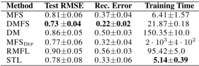
Table 1.Avg. test RMSE, reconstruction error and running time in minutes of each method on the synthetic experiments.
Method Test RMSE Rec. Error Training Time
MFS 0.81±0.06 0.37±0.04 6.41±1.57 DMFS 0.73±0.04 0.22±0.02 21.87±0.18 DM 0.86±0.05 0.50±0.03 150.35±10.0 MFSDEP 0.77±0.06 0.32±0.04 2·10 3± 4·102 RMFL 0.90±0.05 0.56±0.03 95.42±5.0 STL 0.78±0.08 0.33±0.06 5.14±0.39
The results obtained are displayed in Table 1. The best method in terms of the reconstruction error and the RMSE is DMFS, followed by MFSDep and STL. MFS performs
worse than STL. DM and RMFL perform poorly. The differences of DMFS with respect to the other methods are statistically significant (p-value < 5%using a paired Student’s T test). In terms of training time, the fastest method is STL closely followed by MFS and DMFS. DM and RMFL take longer training times due to the expensive grid search procedure that is used to fix their two hyper-parameters. This process demands re-training each method many times. If the optimal hyper-parameters were given, they would be the fastest methods. The training time of MFSDepis very high for the same reason. By contrast,
un-like these methods, DMFS uses Bayesian inference to infer hyper-parameters and does not require any re-training. The better results obtained by DMFS are also explained by Figure3, which shows the average posterior probability that each task and each feature is an outlier, as estimated by DMFS. DMFS successfully identifies tasks4 and8 as outlier tasks and features19and21as outlier features. We note that features 1, 3 and 24 have also a small probability of being outliers. This makes sense because according to Figure2(bottom) they are relevant only for a few tasks.
Probability 1 2 3 4 5 6 7 8 9 10 11 12 0 0.5 1 Probability 1 8 16 24 32 0 0.5 1
Figure 3.Avg. posterior probability forωk= 1(taskkis an
out-lier) andzi= 1(featureiis an outlier) in DMFS, in the synthetic
data. The last prob. is only displayed for the first 32 features. Figure 4 also sheds light on the better performance of DMFS. It shows in a gray scale the average probability that each of the 26 first model coefficients of each task is zero, as estimated by each method. These probabilities are obtained from the approximate posterior in the probabilis-tic models. In DM and RMFL we report the fraction of times that a coefficient is different from zero across exper-iments. We note that DMFS, MFSDep and STL find
pat-terns that agree the most with those of Figure2(bottom). However, STL does not exploit the multi-task setting and is less confident about the non-zeroness of coefficients6to
16for non-outlier tasks. DMFS is also more confident than MFSDep about irrelevant coefficients. On the other hand,
MFS, RMFL and DM give high probability of being differ-ent from zero to coefficidiffer-ents6to16for tasks4and8. The reason is that they assume a few relevant features shared across all tasks and cannot model outlier tasks. Further-more, they also find to be non-zero across all tasks some coefficients corresponding to features that are in fact only relevant for a few tasks (e.g., the coefficients corresponding to features1,3,19,21and24). DM and RMFL can in prin-ciple model some of these coefficients (note that they give higher probabilities of being not zero to some of them), but to avoid their joint selection, these methods would have to shrink non-zero coefficients shared by all non-outlier tasks, producing worse results. In particular, the norms that they use cannot provide very sparse solutions and not shrink rel-evant coefficients (Hern´andez-Lobato et al.,2013).
1 2 3 4 5 6 7 8 9 10 11 12 13 14 15 16 17 18 19 20 21 22 23 24 25 26 1 2 3 4 5 6 7 8 9 10 11 12 Dimension i Task k 1 2 3 4 5 6 7 8 9 10 11 12 13 14 15 16 17 18 19 20 21 22 23 24 25 26 1 2 3 4 5 6 7 8 9 10 11 12 Dimension i Task k 1 2 3 4 5 6 7 8 9 10 11 12 13 14 15 16 17 18 19 20 21 22 23 24 25 26 1 2 3 4 5 6 7 8 9 10 11 12 Dimension i Task k 1 2 3 4 5 6 7 8 9 10 11 12 13 14 15 16 17 18 19 20 21 22 23 24 25 26 1 2 3 4 5 6 7 8 9 10 11 12 Dimension i Task k 1 2 3 4 5 6 7 8 9 10 11 12 13 14 15 16 17 18 19 20 21 22 23 24 25 26 1 2 3 4 5 6 7 8 9 10 11 12 Dimension i Task k 1 2 3 4 5 6 7 8 9 10 11 12 13 14 15 16 17 18 19 20 21 22 23 24 25 26 1 2 3 4 5 6 7 8 9 10 11 12 Dimension i Task k
Figure 4.Average probability for each method across the 100 rep-etitions that each of the 26 first model coefficients of each task is different from zero in a gray scale (0 = white and 1 = black). 5.2. Reconstruction of gene regulatory networks AssumeXis aN×dmatrix with columns denotingdgenes and rows containingN measurements of log mRNA con-centration obtained under different steady state conditions. Consider that X is contaminated with additive Gaussian noise. Then,X ≈ XWT+σ2E, where the entries inE
are standard Gaussian,σ2 is the variance of the noise and
Wis a sparsed×dregression matrix with zero diagonal entries that links the expression level of each gene with that of its transcriptional regulators (Hern´andez-Lobato et al., 2015). When an entry ofWis non-zero there is a regu-latory dependency between the pair of genes it refers to. These dependencies are described by gene regulatory net-works in which there is a node per gene and two nodes are connected with a directed edge if the first gene regulates
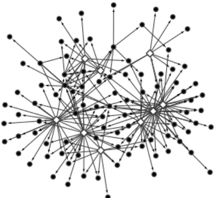
the second. These networks are sparse (with many miss-ing edges) and have hub nodes (transcription factors) that regulate several genes. Figure5shows a sample network.
Figure 5.Sample gene regulatory network used in the experi-ments. Nodes that are potential hubs have a diamond shape.
Table 2.Avg. area under the ROC curve for the network recon-struction experiments and RMSE for the anticancer drug sensitiv-ity experiments, for each of the different methods considered.
Method AUROC RMSE
MFS 0.73±0.05 0.733±0.053 DMFS 0.84±0.05 0.717±0.050 DM 0.76±0.06 0.703±0.050 MFSDEP 0.79±0.05 0.704±0.051 RMFL 0.79±0.05 0.703±0.050 STL 0.70±0.04 0.730±0.049
We formulate the problem of inducing W given Xas a multi-task problem with d tasks where the model coeffi-cients of task k correspond to the k-th row ofW. The design matrixX(k)is given by the matrixXwith column
k set to zero. The targets of taskkare the entries in the k-th column of X. To favor sparse networks we use the proposed prior forW. This prior models the hub nodes in the network by considering jointly relevant features across tasks, but it allows for small deviations to consider genes regulated, in addition, by a few extra genes (outlier fea-tures), or genes regulated by very specific transcription fac-tors (outlier tasks). The regulatory network can be induced by computing the posterior probabilitypij that each entry w(ij) inWis non-zero. The corresponding directed edge j→iis predicted whenpij exceeds a thresholdζ∈[0,1]. Thus, these experiments evaluate the ability of each method to discriminate between relevant and irrelevant coefficients. We evaluate the different methods in the task of inferring gene regulatory networks. The experimental protocol fol-lows the DREAM 4in silicochallenge 2009. We generate 100 networks with 100 genes and sample 90 steady-state measurements from each network using GeneNetWeaver (Schaffter et al., 2011). The reconstruction performance is measured in terms of the area under the ROC curve (AU-ROC) (Fawcett,2006), obtained whenζvaries between 0 and 1. In MFS, DM and RMFL, to induce the network, we
use the absolute values of the estimated entries ofW nor-malized to sum to one, instead of posterior probabilities. Table 2 shows the average AUROC for each method. The best method (higher is better) is DMFS followed by MFSDep, RMFL, DM and MFS. The method with the
low-est performance is STL. The differences are statistically significant (p-value<5%using a paired Student’s T test). This result shows that multi-task methods are beneficial in this problem and that the hypothesis made by DMFS is more adequate, probably because it is more flexible. In DMFS several tasks have a significantly higher probability of being outlier tasks, and the same is observed for several features (results not shown). We have also evaluated here the winning solution of the DREAM 4 challenge (Huynh-Thu et al.,2010). This method uses tree-ensembles to iden-tify relevant features, but does not exploit task relations. The average AUROC obtained is0.75, which is below the one shown in Table2for DMFS, MFSDepand RMFL.
5.3. Denoising of natural images
We consider the problem of denoising the256×256house image used in (Titsias & L´azaro-Gredilla,2011) when it has been contaminated by Gaussian noise. Three levels are considered for the standard deviation of the noiseσ(k).
Namely, 25, 50 and 75,∀k. Following that work, we parti-tion the noisy image in62,001overlapping blocks of8×8
pixels and regard each block as a different task. These tasks are then grouped forming 64 groups of non-overlapping blocks (i.e., one group of32×32blocks,7groups of32×31
blocks,7groups of31×32blocks and49groups of31×31
blocks) which are solved in parallel in a cluster using each multi-task method (see the supplementary material). To de-noise the image we sety(k)equal to each block and each
X(k) equal to an orthonormal basis corresponding to the Haarwavelet. Thus,d= 64andNk = 64for each taskk. It is well known that natural images have sparse represen-tations under a wavelet basis. Thus, the learning process involves finding the wavelet coefficients corresponding to each block from the noisy observations. Using these coeffi-cients the original image can be reconstructed by obtaining their projection under the wavelet basis. We assume in all probabilistic methods the same level of noise for each task. Table 3 shows the peak-signal-to-noise ratio obtained by each method (higher is better) in the denoising process. The best results are obtained by the proposed approach DMFS, which improves the results of the other methods, especially for high levels of noise, where multi-task meth-ods show a clear advantage over single-task learning. As in the previous experiments, DMFS also identifies here sev-eral outlier tasks and features (results not shown). Figure 6 shows the original noisy images and the corresponding denoised images obtained by DMFS for each value ofσ(k).
σ(k)= 25 σ(k)= 50 σ(k)= 75
Denoised
Image
Noisy
Image
Figure 6.Noisy images and corresponding denoised images ob-tained by DMFS, for each different value ofσ(k)considered∀k.
Table 3.Peak-signal-to-noise ratio for each method.
Method σ(k)= 25 σ(k)= 50 σ(k)= 75 MFS 25.90 23.89 23.87 DMFS 30.67 27.25 25.22 DM 28.50 25.91 24.24 MFSDEP 30.46 25.74 23.65 RMFL 28.35 25.56 24.09 STL 30.58 26.37 23.35
5.4. Anticancer drug sensitivity prediction
We consider the dataset described in (Barretina et al., 2012). This dataset contains microarray gene expression data from 479 human cancer cell lines with pharmacologi-cal profiles for 24 anticancer drugs. After removing miss-ing values 294 cell lines remain. We filter the data and consider only the1,000genes with the largest interquartile distance. The task of interest is to predict each drug sensi-tivity (measured in terms of the area over the dose-response curve) from the microarray data for each cell line. Thus, in these experiments d = 1,000, K = 24 andNk = 294
∀k. We use 90% of the data for training and 10% for test-ing. The reported estimates are averaged over100 repeti-tions. We report the test root mean squared error (RMSE). In these experiments assuming in all probabilistic methods the same level of noise for each task also improves results. Table 2 shows the results of the experiments. The best methods are DM, RMFL and MFSDep. The solution of DM
reduces to the one of the group LASSO (i.e., one regular-ization parameters is set always to zero). We believe the better performance obtained by DM and RMFL is a conse-quence of shrinking too much relevant coefficients, which may be useful here to alleviate over-fitting since microarray data is notoriously very noisy. DMFS performs worse than these three methods, and the differences are statistically significant according to a paired Wilcoxon test (p-value <5%). Nevertheless, DMFS improves over the baselines STL and MFS, and the differences are also statistically sig-nificant. Finally, Figure 7 shows the average probability that each drug is an outlier task, as estimated by DMFS.
We observe that several drugs are marked as outlier tasks.
Probability
17
−
AA
G
AEW541 AZD0530 AZD6244 Er
lotinib
Irinotecan L−685458 LBW242 Lapatinib Nilotinib Nutlin
− 3 PD − 0325901 PD − 0332991 PF2341066 PHA− 665752 PLX4720 Paclitax el Panobinostat RAF265 Soraf enib TAE684 TKI258 Topotecan ZD− 6474 0 0.5 1
Figure 7.Avg. posterior probability that each drug is an outlier task, as estimated by DMFS, in the drug sensitivity experiments.
Last, we compare here the utility of DMFS to identify out-lier tasks with that of RMFL. For this, we train the group LASSO on the data when the tasks identified as outliers by each method are removed (recall that the group LASSO performs best). In DMFS we remove those tasks whose probability of being an outlier is above 1%. In RMFL we remove those tasks whose rows inQare not zero. The re-sults obtained indicate that when DMFS is used to remove outlier tasks the RMSE of the group LASSO on the non-outlier tasks is 0.667±0.061, when the outlier tasks are removed, and0.671±0.059otherwise. This improvement is statistically significant according to a paired Wilcoxon test (p-value<5%). By contrast, when RMFL is used to remove outlier tasks the RMSE of the group LASSO on the non-outlier tasks is0.684±0.074, when the outlier tasks are removed, and0.686±0.069otherwise. This other improve-ment is not statistically significant (p-value>5%), which shows that DMFS is better for identifying outlier tasks.
6. Conclusions
Most methods for multi-task feature selection in the liter-ature assume jointly relevant and irrelevant feliter-atures across tasks. This hypothesis may be too restrictive in practice. In this paper, we have proposed a new prior distribution that considers that most tasks share relevant and irrelevant features, but that allows for some tasks to have different relevant and irrelevant coefficients (outlier tasks), and for some features to be arbitrarily relevant or irrelevant for each task (outlier features). This is a more flexible assump-tion. Unfortunately, exact inference is infeasible under such a prior. Nevertheless, a quadrature-free expectation propagation method can be used for approximate inference. A model using our prior has been evaluated in several ex-periments involving the reconstruction of gene regulatory networks, the denoising of natural images and the predic-tion of drug sensitivity from microarray data. These exper-iments show gains in the prediction performance and in the identification of relevant features. Such a prior is also use-ful to better understand the data, since it allows to identify outlier tasks and features. When outlier tasks are removed from the training set, traditional multi-task feature selec-tion methods obtain better results in the non-outlier tasks. This confirms that removed tasks were indeed outlier tasks.
Acknowledgements
Daniel Hern´andez-Lobato gratefully acknowledges the use of the facilities of Centro de Computacin Cientfica (CCC) at Universidad Aut´onoma de Madrid. This author also ac-knowledges financial support from Spanish Plan Nacional I+D+i, Grant TIN2013-42351-P, and from Comunidad de Madrid, Grant S2013/ICE-2845 CASI-CAM-CM. Jos´e Miguel Hern´andez-Lobato acknowledges financial support from the Rafael del Pino Fundation.
References
Argyriou, A., Evgeniou, T., and Pontil, M. Multi-task fea-ture learning. InNeural Information Processing Systems, pp. 41–48. 2007.
Armagan, A., Dunson, D., and Clyde, M. Generalized beta mixtures of Gaussians. InNeural Information Process-ing Systems, pp. 523–531. 2011.
Barretinaet al. The cancer cell line encyclopedia enables predictive modelling of anticancer drug sensitivity. Na-ture, 483:603–307, 2012.
Berger, J. A robust generalized Bayes estimator and confi-dence region for a multivariate normal mean.The Annals of Statistics, 8:716–761, 1980.
Bishop, C. M.Pattern Recognition and Machine Learning. Springer, 2006.
Carvalho, C.M., Polson, N.G., and Scott, J.G. Handling sparsity via the horseshoe. J. Mach. Learn. Res. W&CP, 5:73–80, 2009.
Fawcett, T. An introduction to ROC analysis. Pattern recognition letters, 27:861–874, 2006.
Gong, P., Ye, J., and Zhang, C. Robust multi-task fea-ture learning. InInternational Conference on Knowledge Discovery and Data Mining, pp. 895–903, 2012. Hern´andez-Lobato, D. and Hern´andez-Lobato, J. M.
Learning feature selection dependencies in multi-task learning. InNeural Information Processing Systems, pp. 746–754. 2013.
Hern´andez-Lobato, D., Hern´andez-Lobato, J. M., Helleputte, T., and Dupont, P. Expectation prop-agation for Bayesian multi-task feature selection. In European Conference on Machine Learning, pp. 522–537, 2010.
Hern´andez-Lobato, D., Hern´andez-Lobato, J. M., and Dupont, P. Generalized spike-and-slab priors for Bayesian group feature selection using expectation prop-agation.J. Mach. Learn. Res., 14:1891–1945, 2013.
Hern´andez-Lobato, J. M., Hern´andez-Lobato, D., and Su´arez, A. Expectation propagation in linear regression models with spike-and-slab priors. Machine Learning, 99:437–487, 2015.
Huynh-Thu, V. A., Irrthum, A., Wehenkel, L., and Geurts, P. Inferring regulatory networks from expression data using tree-based methods.PLoS ONE, 5:e12776, 2010. Jalali, A., Ravikumar, P., Sanghavi, S., and Ruan, C. A
dirty model for multi-task learning. InNeural Informa-tion Processing Systems, pp. 964–972. 2010.
Jebara, T. Multi-task feature and kernel selection for SVMs. InInternational Conference on Machine Learn-ing, pp. 55–62, 2004.
Johnstone, I. M. and Silverman, B. W. Empirical Bayes selection of wavelet thresholds. Annals of Statistics, 33: 1700–1752, 2005.
Minka, T. Expectation propagation for approximate Bayesian inference. In Annual Conference on Uncer-tainty in Artificial Intelligence, pp. 362–36, 2001. Mitchell, T. J. and Beauchamp, J. J. Bayesian variable
se-lection in linear regression.Journal of the American Sta-tistical Association, 83:1023–1032, 1988.
Obozinski, G., Taskar, B., and Jordan, M.I. Joint covariate selection and joint subspace selection for multiple clas-sification problems.Statistics and Computing, pp. 1–22, 2009.
Passos, A., Rai, P., Wainer, J., and Daum´e III, H. Flexible modeling of latent task structures in multitask learning. InInternational Conference on Machine Learning, 2012. Schaffter, T., Marbach, D., and Floreano, D. Genenetweaver: In silico benchmark generation and performance profiling of network inference methods. Bioinformatics, 27:2263–2270, 2011.
Seeger, M. Expectation propagation for exponential fami-lies. Technical report, UC, Berkeley, 2006.
Strawderman, W. E. Proper Bayes minimax estimators of the multivariate normal mean.The Annals of Mathemat-ical Statistics, 42:385–388, 1971.
Titsias, M. and L´azaro-Gredilla, M. Spike and slab varia-tional inference for multi-task and multiple kernel learn-ing. In Neural Information Processing Systems, pp. 2339–2347, 2011.
Vogt, J. E. and Roth, V. The group-lasso: `1,∞ regular-ization versus`1,2regularization. In32nd Anual
Sympo-sium of the German Association for Pattern Recognition, volume 6376, pp. 252–261, 2010.
Xiong, T., Bi, J., Rao, B., and Cherkassky, V. Probabilistic joint feature selection for multi-task learning. In Sev-enth SIAM International Conference on Data Mining, pp. 332–342, 2007.
Xue, Y., Liao, X., Carin, L., and Krishnapuram, B. Multi-task learning for classification with Dirichlet process pri-ors.J. Mach. Learn. Res., 8:35–63, 2007.
Zhang, J., Ghahramani, Z., and Yang, Y. Flexible latent variable models for multi-task learning.Machine Learn-ing, 73:221–242, 2008.