Simulations of the Dynamical
Evolution of Compact Groups and
Poor Clusters
by Paul W. Bode
Submitted to the faculty of the University Graduate School in partial fulllment of the requirement
for the degree Doctor of Philosophy in the Department of Astronomy,
Indiana University April 1994
Accepted by the Graduate Faculty, Indiana University, in partial fulllment of the requirements for the degree of Doctor of Philosophy.
Haldan N. Cohn, Co-Chair
Phyllis M. Lugger, Co-Chair Doctoral Committee Richard H. Durisen Andrew D. Bacher April 26, 1994 ii
Vernon and Emily Bode
Acknowledgments
It is a pleasure to thank my advisors, Haldan Cohn and Phyllis Lugger, for their support and guidance during my dissertation work. I must also thank Richard Durisen, who as a teacher and a researcher has enriched my graduate school experience. Thanks also to Andrew Bacher for his interest in my work.
I thank all my fellow graduate students past and present| particularly those who suered through classes with me, Jay White and Bob Grabhorn, as well as my former co-inhabitants at Astro House, Steve Cederbloom, Dave Vesper, Shelby Yang, Brian Pickett, and Glen Spiczak.
Computers being the lifeblood of this project, the work of George Turner in keeping the department system humming along is greatly appreciated.
Indiana University Department of Astronomy
SIMULATIONS OF THE DYNAMICAL EVOLUTION OF COMPACT GROUPS AND POOR CLUSTERS
The eect of dynamical evolution on clusters and their constituent galaxies is examined through simulations of compact groups and poor clusters. The models are fully self-consistent in that each galaxy is represented as an extended structure containing many particles and the gravitational potential arises from the particles alone; the potential is found using the Barnes-Hut \tree" algorithm.
The compact group models contain ve galaxies; a total of N=5000 particles is used to represent both galaxies and a smoothly distributed intra-cluster background. The merging process is found to take longer as less of the cluster mass is put into the galaxy halos; this delay is consistent with the lengthening of the dynamical friction time scale as galaxy masses are reduced.
The N=40,000 cluster models contain 50 galaxies. Those models with half of the mass initially contained in the background all followed a similar pattern of behavior. In 10 Gyr, merging has resulted in the formation of a dominant,
slowly-moving, centrally located galaxy. No high peculiar-velocity brightest cluster galaxies (which are observed in 10% of clusters) are produced in these
models. The cluster density prole around the rst-ranked galaxy (FRG) becomes strongly cusped and resembles a singular isothermal sphere; this is accompanied by an increase in the number of multiple nuclei seen in the FRG. Many observed
properties of poor clusters (including M12, FRG luminosity, and the frequency
of multiple nuclei) can best be t by cluster models with ages 11 Gyr, with the
exception that tting observations of the peculiar velocities of the FRG requires younger ages of 8 Gyr.
Increasing the background mass fraction to 75% slows the rate of merging, but otherwise causes little change in behavior. For a fraction of 90%, the onset of merging can be delayed for over 13 Gyr; thus a dominant central galaxy is not created.
Contents
1 Overview
1
2 Regions of High Galaxy Density
5
1. Relevant Physical Processes : : : : : : : : : : : : : : : : : : : : : : : 6 1.1. Violent Relaxation and Virialization. : : : : : : : : : : : : : : 6 1.2. Two-Body Relaxation : : : : : : : : : : : : : : : : : : : : : : 7 1.3. Dynamical Friction : : : : : : : : : : : : : : : : : : : : : : : : 7 1.4. Collisional Stripping : : : : : : : : : : : : : : : : : : : : : : : 8 1.5. Merging : : : : : : : : : : : : : : : : : : : : : : : : : : : : : : 9 1.6. Tidal Limitation : : : : : : : : : : : : : : : : : : : : : : : : : 9 2. Compact Groups : : : : : : : : : : : : : : : : : : : : : : : : : : : : : 10 3. Clusters of Galaxies : : : : : : : : : : : : : : : : : : : : : : : : : : : : 13 3.1. Theoretical Background : : : : : : : : : : : : : : : : : : : : : 13 3.2. Observational Background : : : : : : : : : : : : : : : : : : : : 15 vii
3 The N-Body Tree-Code
18
1. N-Body Methods : : : : : : : : : : : : : : : : : : : : : : : : : : : : : 19 2. The Barnes-Hut Algorithm : : : : : : : : : : : : : : : : : : : : : : : : 20 3. Modications to Hernquist's Code : : : : : : : : : : : : : : : : : : : : 22
4 The Compact Group Models
25
1. Introduction : : : : : : : : : : : : : : : : : : : : : : : : : : : : : : : : 26 2. The Models : : : : : : : : : : : : : : : : : : : : : : : : : : : : : : : : 26 3. The Evolutions : : : : : : : : : : : : : : : : : : : : : : : : : : : : : : 29 4. Physical Processes : : : : : : : : : : : : : : : : : : : : : : : : : : : : 33 5. Group Properties : : : : : : : : : : : : : : : : : : : : : : : : : : : : : 37 6. Groups of Ten Galaxies : : : : : : : : : : : : : : : : : : : : : : : : : 47 7. Summary : : : : : : : : : : : : : : : : : : : : : : : : : : : : : : : : : 48
5 The Cluster Models
51
1. Introduction : : : : : : : : : : : : : : : : : : : : : : : : : : : : : : : : 52 2. The Cluster Models : : : : : : : : : : : : : : : : : : : : : : : : : : : 52 3. The Evolutions : : : : : : : : : : : : : : : : : : : : : : : : : : : : : : 59 4. Merging : : : : : : : : : : : : : : : : : : : : : : : : : : : : : : : : : : 65 5. The Mass Function : : : : : : : : : : : : : : : : : : : : : : : : : : : : 68 6. Mass Segregation : : : : : : : : : : : : : : : : : : : : : : : : : : : : : 70
8. The Density Distribution : : : : : : : : : : : : : : : : : : : : : : : : : 77 9. Multiple Nuclei : : : : : : : : : : : : : : : : : : : : : : : : : : : : : : 83 10. Summary : : : : : : : : : : : : : : : : : : : : : : : : : : : : : : : : : 88
6 Conclusions
90
1. Compact Groups : : : : : : : : : : : : : : : : : : : : : : : : : : : : : 91 1.1. Discussion : : : : : : : : : : : : : : : : : : : : : : : : : : : : : 91 1.2. Conclusions and Future Directions : : : : : : : : : : : : : : : 94 2. Clusters : : : : : : : : : : : : : : : : : : : : : : : : : : : : : : : : : : 95 2.1. Comparison With Other Simulations : : : : : : : : : : : : : : 95 2.2. Comparison With Observations : : : : : : : : : : : : : : : : : 98 2.3. Richer Clusters and Substructure : : : : : : : : : : : : : : : : 101 2.4. Conclusions and Future Directions : : : : : : : : : : : : : : : 102REFERENCES
104
List of Tables
4.1 Model Parameters for N=5000, 5 Galaxy Groups : : : : : : : : : : : 28 5.1 Parameters for 50-galaxy models: : : : : : : : : : : : : : : : : : : : : 56 5.2 Galaxy Parameters : : : : : : : : : : : : : : : : : : : : : : : : : : : : 57
List of Figures
4.1 Snapshots from a typical run. : : : : : : : : : : : : : : : : : : : : : : 30 4.2 The number of galaxies as a function of time. : : : : : : : : : : : : : 32 4.3 The radial trajectories of the galaxies. : : : : : : : : : : : : : : : : : 34 4.4 The total number of particles bound to galaxies. : : : : : : : : : : : : 36 4.5 Apparent virial quantities: (a) radius (b) velocity (c) mass (d)
crossing time. : : : : : : : : : : : : : : : : : : : : : : : : : : : : : : : 38 4.6 The distribution of (a) median two-dimensional separations, (b)
line-of-sight velocity dispersions, (c) crossing times.: : : : : : : : : : : : : 43 4.7 The number of galaxies as a function of time for 10-galaxy groups. : : 49 5.1 The initial conguration of a typical model. : : : : : : : : : : : : : : 53 5.2 Snapshots showing the luminous portion of a =50 model. : : : : : : 60 5.3 Snapshots showing the entire galaxies of a =50 model. : : : : : : : : 61 5.4 Same as 5.2 but for =50. : : : : : : : : : : : : : : : : : : : : : : : : 62 5.5 Same as 5.3 but for =75. : : : : : : : : : : : : : : : : : : : : : : : : 63
xii 5.6 Snapshots showing the entire galaxies of a =90 model. : : : : : : : : 64 5.7 The number of galaxies as a function of time for =50. : : : : : : : : 66 5.8 The number of galaxies as a function of time for all . : : : : : : : : 67 5.9 The luminous mass function. : : : : : : : : : : : : : : : : : : : : : : : 69 5.10 The distance of the FRG from the cluster center. : : : : : : : : : : : 72 5.11 Cumulative distribution of Z-scores. : : : : : : : : : : : : : : : : : : : 75 5.12 Three-dimensional galaxy number density. : : : : : : : : : : : : : : : 78 5.13 Surface galaxy number density. : : : : : : : : : : : : : : : : : : : : : 80 5.14 Surface galaxy number density in the ln | R plane. : : : : : : : : : 82 5.15 The percentage of FRG with secondary nuclei. : : : : : : : : : : : : : 84
Chapter 1
Overview
CHAPTER1. OVERVIEW 2
Studies of the distribution of luminous matter in the universe indicate that galaxies are clustered on a wide range of scales, from binaries and compact groups only slightly larger than the galaxies themselves to sheets or walls extending over distances as large as can presently be observed. Roughly 5% of all galaxies are in groups or clusters with a density > 1 galaxy-Mpc?3 (Dressler 1984). Groups of
galaxies, such as the Local Group, contain up to about 30 galaxies, and clusters contain more than this| very rich clusters, such as the nearby Virgo Cluster, may contain thousands of galaxies.
There are a number of reasons to study groups and clusters in addition to their prominent optical structure. The formation and evolution of a galaxy will depend on its environment, so observations of galaxies in a given cluster can reveal facets of the evolution of individual galaxies, much as the study of stellar populations in open and globular clusters has been used to elucidate stellar evolution. Clusters have large mass-to-light ratios, so they may be used as probes of dark matter, particularly since many clusters are also bright in the X-ray band. Clusters and galaxies in clusters are often used as standard candles and tracers of large-scale structure; it is thus necessary to know how to correct for secular evolution in clusters. Furthermore, large clusters may maintain some memory of their initial conditions, making their current structure a possible test of cosmological models.
Galaxies will interact with each other and their environment, changing the properties of both clusters and individual galaxies. Despite intensive observational and theoretical study of clusters of galaxies, there are many unresolved questions concerning the eect of this dynamical evolution on clusters and their constituent galaxies. The cores of clusters are thought to be virialized (see Section 1.1.); many dynamical processes operate once equilibrium has been reached. These
include interactions between galaxies and the dark-matter component of the cluster via dynamical friction and galaxy-galaxy interactions via two-body relaxation, merging, and tidal stripping. If there is signicant substructure in clusters, then the overall cluster potential will evolve on a dynamical timescale and mean-eld relaxation will also be an important process. The properties of the rst-ranked galaxy (FRG) in a cluster may be aected by these processes; for recent reviews see Lugger (1991), Richstone (1990), and Merritt (1988). Simulations of the dynamical interaction of galaxies in clusters have produced conicting results, as discussed in Section 3.1.
The dynamical state of compact groups (as dened in Section 2.) has also long been a subject of controversy. Computer simulations of group evolution suggest that groups have short lifetimes, with all of the member galaxies merging together to form a single massive galaxy on a time scale short compared with the age of the universe. This theoretical prediction is confronted with discordant observations, including: (1) while groups of galaxies are thought to have formed early in the life of the universe, there are many compact groups still observed at the present time, and (2) there are very few isolated supergiant galaxies of the sort that would be produced by the \merger instability" of groups.
Computer simulations of the evolution of clusters have tended to split the problem into separate computations of: (1) approximate cross-sections for galaxy interactions, and (2) cluster evolution with point-mass galaxies interacting according to these cross-sections. A unied treatment which directly simulates the evolution of a cluster of realistic, extended galaxies is clearly preferable since galaxies are continuously undergoing interactions. Such a treatment was previously impractical because of the need to limit computational expense, but it is now possible to revisit this subject with substantially more computational power than
CHAPTER1. OVERVIEW 4
has heretofore been available. This approach provides higher resolution, allowing simulations with a degree of physical realism beyond what has previously been possible in this area. This is a relatively new but growing technique; Funato, Makino, and Ebisuzaki (1993) have carried out cluster evolutions in this manner using a special-purpose computer, and Barnes (1992) reported one cluster model made on a standard workstation.
This thesis presents a number of N-body models of compact groups and clusters. The models are fully self-consistent in that each galaxy is represented as an extended structure containing many particles and the gravitational potential arises from the particles alone. In Chapter 2 an overview of the relevant physical processes is given and recent observational and theoretical work is reviewed; Chapter 3 describes the code employed for the simulations. Chapters 4 and 5 gives results for compact groups and clusters, respectively. Finally, these results are discussed in Chapter 6.
Note that a Hubble constant of H0 = 50 km s
?1 Mpc?1 is used throughout
Chapter 2
Regions of High Galaxy Density
CHAPTER2. REGIONSOF HIGHGALAXYDENSITY 6
1. Relevant Physical Processes
Like the stars in a globular cluster, galaxies in a group or cluster will undergo gravitational scattering; the process is much more complicated for galaxies, however, since the internal degrees of freedom come into play in a typical galaxy-galaxy interaction. This is a result of the fact that the physical sizes of galaxies are comparable to the typical intergalaxy separation. In addition, galaxies will interact with the dark matter component of clusters, which represents as much as 90% of the cluster mass. While the presence of this dark matter is evidenced by its contribution to the cluster gravitational potential, the nature of the dark matter is unknown. Possible dark matter constituents include very low mass stars and brown dwarfs, stellar remnants including black holes, and weakly interacting massive subatomic particles. In addition to being responsible for the high velocity dispersion of the galaxy distribution in the cluster (1?210
3 kms?1), the dark
matter also exerts a dynamical friction drag on galaxies, which causes their orbits in the cluster potential well to decay. Interaction between galaxies and the dark matter background is expected to result in evolution of the spatial distributions of both of these components of clusters. A summary of the relevant dynamical processes is given below. Other physical processes not mentioned here may also be important, such as ram pressure stripping or gas evaporation.
1.1. Violent Relaxation and Virialization.
The initial collapse of a cluster out of the Hubble ow randomizes the orbital velocities of the galaxies. A given point in the collapsing system will experience a strongly uctuating gravitational potential; thus the interaction of galaxies with
the mean tidal eld causes the virialization of the system. This will occur on the scale of the collapse time of the system, which in rich clusters is short compared to the Hubble time. For example, the Coma cluster has a mass M 10
15h?1M and
a size R1h
?1Mpc, so the collapse time
c is roughly c R3=GM 1=2 10 9yr (2:1)
or a tenth of a Hubble time.
1.2. Two-Body Relaxation
Galaxy-galaxy interactions will tend to randomize the kinetic energies of the galaxies in a cluster. As in an ideal gas, there will be an equipartition of kinetic energy between mass groups. Since after virialization the orbital velocity is independent of the mass, the more massive galaxies will on average have greater kinetic energy; two-body relaxation will thus cause the more massive galaxies to lose kinetic energy to the less massive ones. This in turn means that mass segregation will occur in the cluster | the more massive group will be concentrated towards the center in lower-energy orbits.
1.3. Dynamical Friction
As a special case of two-body relaxation, a massive object moving through a background of less massive, more slowly moving eld objects will be slowed down. This is because the eld objects will be gravitationally attracted towards the massive body as it moves by, thus creating a gravitational wake behind this body. The size of the wake thus created will be proportional to the mass of the body, M.
CHAPTER2. REGIONSOF HIGHGALAXYDENSITY 8
The force between the massive object and the region of overdensity behind it is thus / M
2. In the limit of the background objects being much less massive than
the test object, an accurate estimate of the eect of dynamical friction is given by the Chandrasekhar formula (Binney and Tremaine 1987, x7.1):
d~v
dt =?4G
2bMf(v)ln
v3 ~v (2:2)
where f(v) depends on the test object velocity v as compared to the dispersion of the background objects, and depends on the ratio of test to background object mass. Thus the change in velocity scales as dv=dt ?bMv
?2. As one might
expect, dynamical friction is most pronounced for slower-moving, more massive objects moving through a denser background.
1.4. Collisional Stripping
Close encounters between galaxies can result in mass being stripped from them, because of the tidal forces they exert on each other. This can be seen in the case of a perturbing body of massMp moving past a galaxy of massMg which is at
rest. For a high-speed encounter (where the perturber's velocityV is much larger than the velocity dispersion of the galaxy hvgi) which is not too close (b > 5r,
where b is the impact parameter and r is the mean radius of the galaxy), the change in the internal energy of a disk galaxy is (Binney and Tremaine 1987, x7.2)
E = 43G2M 2
pMgr2
b4V2 . (2:3)
Since E > 0, the galaxy becomes less bound. Slow, close encounters will have the greatest eect. Stars on nearly unbound orbits may receive a large enough kick from the perturber to break free of the galaxy; numerical studies indicate that the amount of mass lost is quite sensitive to the mass distribution of the galaxies (see the discussion in Mamon 1987).
1.5. Merging
Since energy is conserved, the increase in internal energy due to tidal forces is matched by a decrease in the kinetic energy of the perturbing galaxy. If E due to the encounter is larger than the relative orbital energy of the galaxies, then the two will become bound and will eventually merge. Merging is most likely for close encounters (b on the scale of the galaxy sizes) which are slow (the relative velocity roughly equal to the galaxy velocity dispersions). Once galaxies begin merging, the relevant time scale is the stellar orbital period ( 10
8 yr), so the
merger product will quickly reorganize itself into a new equilibrium conguration. In N-body experiments, the product of a merger is elliptical (either prolate for head-on encounters or oblate for encounters with larger angular momentum; see Binney and Tremaine 1987, x7.4). This may not always be the case for real
galaxies| disk galaxies with counter-rotating cores or counter-rotating gas and stellar components have be found, and the formation mechanism for such an object may include merging.
1.6. Tidal Limitation
Galaxies within a cluster will experience a tidal force from the mean gravitational eld of the cluster itself. This will limit the size of the galaxy; for a circular orbit near the cluster center this is analogous to a Roche limit. For a cluster with core radius RC and dispersion V , a galaxy will have a size less than
the tidal radius
RT = R2Chvgi
CHAPTER2. REGIONSOF HIGHGALAXYDENSITY 10
(Merritt 1984). For a rich cluster RT ' 50kpc. However, numerical experiments
indicate this may not be a good estimate for elliptical orbits; such galaxies are near their pericenter for only a fraction of an orbital time, and thus may not be as severely limited as galaxies on circular orbits.
2. Compact Groups
Compact groups of galaxies have generated much interest and debate in recent years. As cataloged by Rose (1977) and Hickson (1982), compact groups are observationally identied as isolated congurations of galaxies with a high surface density contrast above the background. In particular, Hickson (1982) required that a compact group fulll three criteria:
Population: 4 or more galaxies
Compactness: surface brightness inside the smallest circle containing the
galaxies < 26:0 mag arcsec?2
Isolation: N 3G, where N and G equal the angular diameters of the
smallest circle containing the group and the largest circle containing no other galaxy, respectively.
Observational evidence indicates these are true physical associations: > 30% of member galaxies show optical distortions and > 50% show kinematic distortions, some groups have substantial intergalactic gas and stars, and the groups are more centrally concentrated than chance alignments would be.
These observations prompt the expectation of a rapid rate of dynamical evolution in compact groups. Their high densities and low velocity dispersions,
corresponding to crossing times of order 0.1 Gyr, indicate that dynamical eects, such as tidal stripping and merging, should cause a signicant change in structure within a fraction of a Hubble time.
Numerical models support this view; they generally show that galaxies in a compact conguration will rapidly merge together into a single large remnant. The rst attempt to self-consistently model groups was made by Carnevali et al. (1981). Each of their galaxies consisted of 20 gravitationally bound mass points; the cluster of 10 or 20 galaxies was initially virialized. They found a `merging instability'| extensive merging in a few dynamical times| which proceeded up to the formation of a large central object.
Barnes (1985) rened and extended this approach. His galaxy models were gravitationally bound equilibrium congurations (King models) of equal mass particles; some particles at the core of the galaxy were identied as luminous and the remainder represented dark matter. The dark particles were given a softening length four times that of the luminous ones. Five galaxies were placed with random position and velocity in a cluster, and in some cases additional dark particles were placed in a common group background; a total of N=1500 particles was used. Models were run with groups initially virialized, expanding, or near maximum expansion. This study also found rapid merging. For expanding models, the subsequent collapse triggered a burst of merging, leaving a single remnant after roughly 3 dynamical times. Virialized groups lasted somewhat longer, as did groups with a larger amount of material in the common background; however, even groups with 75% of the mass in the background were reduced to two galaxies within 4{5 crossing times.
CHAPTER2. REGIONSOF HIGHGALAXYDENSITY 12
These simulations suggest that compact groups should exist for only a fraction of a Hubble time; however, this is dicult to reconcile with some observational results. Assuming that the merger remnant would be identied as an early-type galaxy, a high merger rate is inconsistent with the nding that the fraction of late-type galaxies in compact groups diers only marginally from that in the eld (Hickson, Kindl, and Huchra 1988). Also, Hickson's sample was chosen in part on the basis of isolation. Sulentic (1987) found that Hickson's groups fell in regions of relatively low galaxy surface density (near the eld density), and Rood and Williams (1989) conrmed that two-thirds of these groups have neighborhoods containing no more galaxies than expected from the superposition of eld galaxies. However, there are very few isolatedbright elliptical galaxies of the sort that would be produced by the merging instability. One possible resolution of these diculties would be a lower merger rate in compact groups. In fact, there is observational evidence that the merger rate is lower than might be expected from their short crossing times. Zepf (1993) concludes from various measures of the number of ongoing mergers that merging occurs on a time scale signicantly longer than the crossing time.
One way to achieve a lower merger rate is to alter the distribution of dark matter. Hickson, et al. (1992, hereafter HMHP) have concluded that more than 85% of the mass in compact groups could be nonluminous. In simulations it is often assumed that all of the mass in the group is attached to the galaxies; if instead the dark matter is distributed throughout the group in a common background then a lower merger rate would result. The possibility that the dark matter distribution is not concentrated around galaxies is supported by the X-ray observations of the NGC 2300 group by Mulchaey, et al. (1993); they found a symmetric gas distribution not centered on any galaxy, and estimated that baryons can account for
only 4% of the mass needed to gravitationally bind this gas. However, Henriksen
and Mamon (1994) argue that this estimate is sensitive to the temperature prole of the gas and the radius out to which the X-rays are detected; they nd that baryons account for > 20% of the mass of the group. Ponman and Bertram (1993) observed a similar cloud centered on a group from Hickson's catalog, and they estimated the baryon fraction to be >13%.
In simulations it is often assumed that all of the mass in the group is attached to the galaxies; if instead the dark matter is distributed throughout the group in a common background, then a lower merger rate would result. In Chapter 4 a set of N-body models of compact groups with a wide range in the initial background mass fraction is presented which test this possible resolution to the diculties presented by compact groups.
3. Clusters of Galaxies
3.1. Theoretical Background
The observation that some clusters contain a central, giant cD galaxy has led to the theory that this galaxy achieved its present size by \cannibalizing" other galaxies over the life of the cluster. The original prediction of galactic cannibalism rates in rich clusters (Ostriker and Tremaine 1975, Hausman and Ostriker 1978) is based on a highly approximate theory that uses average interaction rates for galaxies in a cluster core without considering actual galaxy trajectories; these interaction rates were sampled using Monte-Carlo techniques in the latter study. These studies predicted high galactic cannibalism rates in rich (N 10
3),
high-velocity-dispersion clusters ( 10
CHAPTER2. REGIONSOF HIGHGALAXYDENSITY 14
(FRG) growing by> 10L over the cluster lifetime.
The more detailed simulations by Richstone and Malumuth (1983) and Malumuth and Richstone (1984) followed the trajectories of individual galaxies moving in a xed background containing 85% of the cluster mass, while still using a Monte Carlo treatment of galaxy-galaxy interactions. Internal galactic structure was not resolved; instead, cross-sections derived from other simulations of galaxy collisions were used to model merging and tidal stripping. Roughly 25% of a set of dierent realizations of the same initial conditions were found to produce a cD galaxy, independent of cluster richness. This suggests that statistical uctuations play an important role in determining the morphological types of clusters. Stripping did reduce most galaxy luminosities. If a large central galaxy was present, it would accrete this material, thereby increasing the luminosity of its halo.
Merritt (1983, 1984) arrived at conclusions that are in striking contrast to the preceding results, based on a statistical description of the galaxy orbital energy and mass distribution and a Fokker-Planck treatment of the evolution of these distributions due to interactions. He found that no signicant tidal stripping occurs due to galaxy-galaxy interactions after the period of cluster formation and that galaxy mergers do not occur at a signicant rate in rich, virialized clusters. This is a result of strong truncation of galaxies by the mean tidal eld of the cluster, which results in galaxies having smaller initial size and thus smaller interaction cross-sections. Merritt (1988) thus concludes that, contrary to the \strong" cannibalism hypothesis (i.e., that cD galaxies are produced by merging), the morphology of the FRG is xed during early stages of cluster evolution and subsequently only \weak" cannibalism occurs, whereby the FRG undergoes only a modest increase in luminosity of a few L. Merritt suggests that merging may
form present-day, rich clusters.
3.2. Observational Background
As reviewed by Lugger (1991), a number of observational investigations over the past decade have sought to test the galactic cannibalism theory by investigating the properties of cluster galaxies and their spatial and kinematic distributions within the cluster. Overall, these studies suggest that the eects of dynamical evolution on rich clusters are more subtle than originally predicted. FRG's that are classied as D and cD appear to represent the bright end of the distribution of \normal" FRG's in observed properties, rather than a separate population. This suggests that the same mechanisms | which may include galaxy merger | play a role in the formation and evolution of all FRG's. The improved evolutionary simulations that we report here will allow more specic tests for the eects of dynamical evolution in clusters.
The observation of multiply-nucleated FRG's is frequently cited in support of the galactic cannibalism picture. The FRG in as many as 50% of all clusters contains one or more secondary nuclei, i.e. smaller galaxies within 20 kpc (using Hubble constant H0 = 50 km s
?1 Mpc?1) projected distance of the nucleus of the
dominant galaxy (Hoessel and Schneider 1985). The cannibalism picture predicts that the FRG will have satellite galaxies on decaying circular orbits with circular velocities of less than 300 km s?1 and orbital radii of 10{20 kpc. Cowie and Hu
(1986) analyzed the observed distribution of velocities of 75 secondary nuclei relative to the FRG; they nd that the distribution of these velocities is best t with a two-component Gaussian model in which 60% of the satellites belong to a low-velocity-dispersion population bound to the FRG and the remainder
CHAPTER2. REGIONSOF HIGHGALAXYDENSITY 16
belong to the normal core population of the cluster which has a higher velocity dispersion. Bothun and Schombert (1990) obtained a complete sample of velocities from the inner 600 kpc of 8 clusters; the combined sample was also well t by a double Gaussian, but with 20% of the galaxies belonging to the bound population. They argue that these galaxies are moving on highly elongated orbits, since this population would quickly disappear due to dynamical friction if the galaxies were on circular orbits; a similar conclusion was reached by Tonry (1985).
The practice of combining data from clusters with dierent velocity dispersions has been criticized by Gebhardt and Beers (1991), who point out that the sum of a number of Gaussians with dierent dispersions leads to a distribution which is not a Gaussian, but rather is more strongly peaked at low velocities. This is not a diculty in the approach taken by Lauer (1988), who used photometric data for the central regions of 16 clusters to assess evidence for physical interaction between the nuclei. Half of the sample showed photometric distortions indicative of interaction. These distortions were seen in systems with both large velocity dierences between the nuclei (> 1000 km s?1) and small dierences (< 300 km
s?1); only the latter group are consistent with cannibalism. Lauer estimates that
the central galaxy increases in luminosity by 2L in 5 Gyr; since a typical cD galaxy
has a total luminosity ' 10L
, this is consistent only with weak cannibalism.
Similarly, Merrield and Kent (1991) compute a rate of growth of the central galaxy of only 1L per 10 Gyr, and nd no evidence for a bound population when
comparing the velocity distribution of cluster members projected within 20 kpc of the central dominant galaxy with the distribution for control samples drawn from further out in the clusters.
One recent observational development is the discovery of a number of cD galaxies with peculiar velocities larger than the velocity dispersion of the cluster in
which they are found (e.g. Zabludo et al. 1993, Bird 1994). To investigate whether this is possible in the strong cannibalism picture, Malumuth (1992) improved on the scheme of Malumuth and Richstone (1984) by following galaxy orbits in an N-body fashion to identify collision and merging events; only 19% of models with half of the mass in the background formed a cD, a considerably lower rate than seen in the earlier study. Furthermore, the peculiar velocities of the cD galaxies, which decay over time, were too low at the end of the simulations to be consistent with the observed distribution, implying that cD galaxies and/or the clusters in which they are found were formed relatively recently.
In Chapter 5 a set of cluster models is presented. These will show that merging can create a dominant central FRG, at least in poor clusters. The properties of the FRG thus produced (including peculiar velocities and multiple nuclei frequency) provide a test of the cannibalism picture.
Chapter 3
The N-Body Tree-Code
1.
N-Body Methods
Given the complexity of self-gravitating systems, some form of numerical integration becomes necessary to examine their time-dependent behavior. Generally a Monte-Carlo technique, whereby N particles are used to sample the stellar distribution function, is used. The computationally expensive part of N-body simulations is nding the gravitational potential at each step. To do this directly, one must nd the force between each pair of particlesi and j:
~Fij = Gmimj
j~xj ?~xij 3 (~xj
?~xi) (3:1)
This direct method is extremely exible, but for a signicant number of particles it becomes too time consuming, since the number of pairs and hence the computational cost scales as O(N
2). Thus for large N it is more practical to use
an approximate method to compute the potential.
Approximate methods in which the computational cost scales as O(N)
have been developed. One class is multipole expansion methods, for example the Self-Consistent Field (SCF) method (Hernquist and Ostriker 1992), in which the potential is calculated as an expansion in some set of basis functions. One must calculate the contribution of each particle to the gravitational eld, so calculating the expansion coecients involves a sum over all particles rather than over all pairs. This method is especially well suited for massively parallel computers (Yang et al. 1994). However, this method requires a suitable set of basis functions, such that only the rst few terms are needed to give an accurate approximation. Thus expansion methods are most useful for spherical, centrally concentrated systems.
Another frequently used technique is the Particle-Mesh (PM) method; codes employing this technique scale as O(N) or O(N log N). Here space is divided by
CHAPTER3. THEN-BODYTREE-CODE 20
a mesh or grid which is used for the potential computation. The positions of the particles are used to nd the density at the grid points, the potential is computed at the grid points, and then the potential is extrapolated from the grid points back to the particles. Ecient techniques involving the use of discrete Fourier transforms have been developed for the potential computation step of this method. PM techniques may be inappropriate for inhomogeneous systems with large density contrasts, because if some volume of space is devoid of particles, the corresponding portion of the grid will be superuous. Also, the overall resolution is limited by the grid size. This has led to the development of hybrid techniques which compute both the short-range force between nearby particles and the long-range force on the grid, as well as adaptive grid techniques which increase the grid resolution in denser regions. The Barnes-Hut algorithm described below is in the spirit of these latter techniques.
2. The Barnes-Hut Algorithm
Codes employing the Barnes-Hut (1986) algorithm are often referred to as \tree codes" because a tree data structure is usually employed. Rather than use a simple, xed spatial gridding, the tree algorithm uses a many-level partitioning hierarchy of cells within cells which is organized using a tree data structure. Computing the force on a given particle involves traversing the tree to increasing depth to determine which particles to treat directly and which to include as members of distant cells. The evolutions presented here were carried out using a modied version of a a fully vectorized tree code (Hernquist 1987, Hernquist 1990, Makino 1990) kindly supplied by Lars Hernquist. The great advantage of using a tree-code is that it reduced the task of computing the potential of an N-body
system to an O(N log N) operation, while at the same time being well suited for
simulating inhomogeneous systems with little spatial symmetry such as galaxy clusters. Hernquist's (1987, 1990) tests indicate that the tree-algorithm is the most ecient method for simulating systems which do not admit a high degree of spatial symmetry when N exceeds a few thousand. Thus is it the algorithm of choice for our investigation.
In this code, space is partitioned into an hierarchy of cubical cells. The `root' of the tree is a cell which contains all of the particles. This root has eight `branches' corresponding to the bisection of the root cell along each dimension, creating eight smaller cubical subcells. This subdivision is iterated, corresponding to further branching of the tree. The process is continued for each cell that contains more than one particle; thus the branching of the tree ends at `leaves' corresponding to individual particles.
To compute the gravitational force on a given test particle, the contents of a cell can be approximated as a point with mass equal to the sum of all the masses inside the cube and position equal to their center of mass; this approximation is more accurate the farther the cell is from the test particle. If greater accuracy is needed, the cell can be divided into its eight smaller subcells. The force calculation thus involves a tree traversal; each node is tested against some tolerance criterion, and either that cell is used or one moves further along the tree. Using the standard Barnes-Hut algorithm, a cell is used only if
d > s= (3:2)
where d is the distance from the particle to the center of mass of the cell, s is the size of the cell, and is a xed tolerance parameter; if the cell does not satisfy this criterion, the eight subcells are examined.
CHAPTER3. THEN-BODYTREE-CODE 22
The positions and velocities are updated using a standard leapfrog integrator, which is accurate to second order in the time step. Since long-range forces are computed approximately, there is no advantage in using a higher-order integrator. Another consequence of approximation is that energy and momentum will not be exactly conserved, since the approximate forces are not guaranteed to be symmetric. However, for reasonable values of and of the time step, this source of nonconservation is comparable that to due to truncation errors in the time integrator (Hernquist 1987).
3. Modications to Hernquist's Code
In most N-body simulations it is not desirable for the particles to behave like point masses, since one is sampling a more continuous distribution. Therefore most simulations use a \softened potential". For example, one popular method is to alter equation 3.1 to ~Fij = ( Gmimj j~xj ? ~xij 2+2) 3=2(~xj ?~xi) (3:3)
where is known as the softening length. This length gives a lower limit on the scale of particle clustering. Equation 3.3 can be derived analytically as the force between a point mass and a Plummer sphere with a core radius of .
In the tree code, gravitational interactions for separations of less than 2 are softened using a cubic spline kernel. For separations larger than 2 the force is that of equation 3.1. For smaller separations the force is equation 3.1 evaluated at r = 2 and multiplied by a factor which is less than unity. This factor is a function of on the separation; details are given in Hernquist and Katz (1989) or Dyer and Ip (1993). If the force is being calculated for two particles with dierent softening lengths, the larger is used.
The use of softening in the tree code can introduce a source of error (Hernquist 1987). When using equation 3.2, it is possible that a cell will not be opened even though it contains a particle within 2 of the particle for which the force is being calculated; i.e., a sphere of radius 2 centered on this latter particle could still intersect with some portion of the cell's volume even though d > 2s. If this happens the interaction of the two particles will not be properly softened. Therefore, the above criterion was replaced by one which guarantees that only cells which could not possibly contain particles within 2 of the particle under consideration are used, namely:
d > 2 +p
3s (3:4)
Requiring that this inequality holds ensures that the entire cell is further than 2 away from the particle, even if the center of mass is in the furthest corner of the box. If more than one softening length is used in a simulation, the longest is the one used in equation 3.4.
It might be asked if there are situations where cells would be opened when using equation 3.2 but not equation 3.4; this would make the criterion used here less accurate than the Barnes-Hut method. In such a case d < s= but d > p
3s; this is not possible for > 1=p
3'0:577. Thus the method used here is at least as
accurate as the Barnes-Hut method with = 0:577 and generally more so, at the expense of having to calculate a greater number of force terms. This becomes more obvious if we rewrite equation 3.4 as
d?2 > s=(1= p
3) (3:5)
Useful values for the tolerance parameter are 0:3 1:0 (Hernquist 1987), since
must be small enough to provide accurate force calculations but not so small that an unreasonable number of force terms is included. While employing equation 3.4
CHAPTER3. THEN-BODYTREE-CODE 24
does increase the number of force terms used, this method avoids the introduction of an additional loop in the frequently used subroutine which creates interaction lists; this routine already accounts for almost half the CPU time consumed by the code. Also, using = 1=p
3 avoids the pathological situation described by Salmon and Warren (1994), which can lead to large systematic errors.
Hernquist specically optimized the code for the Cray Y-MP environment using Cray-specic routines. These were eliminated so that the code could run on several dierent machine architectures. However, with newer Fortran compilers the code still vectorizes, and this change actually had the eect of improving the performance of the code on a Cray Y-MP. Quadrupole corrections to the gravitational force were not used, since they would not signicantly increase the accuracy (Hernquist 1987), so that portion of the code was excised. These changes improved the speed of the code by roughly a factor of two and reduced the memory requirements.
Chapter 4
The Compact Group Models
CHAPTER4. THECOMPACT GROUP MODELS 26
1. Introduction
As discussed in Section 2., a possible resolution to the questions surrounding compact groups could be that there is a merging rate lower than might be expected from the short crossing times. One way to achieve a lower merger rate is to alter the distribution of dark matter. In simulations it is often assumed that all of the mass in the group is attached to the galaxies; if instead the dark matter is distributed throughout the group in a common background, then a lower merger rate would result. This chapter presents a set of N-body models of compact groups with a wide range in the initial background mass fraction.
2. The Models
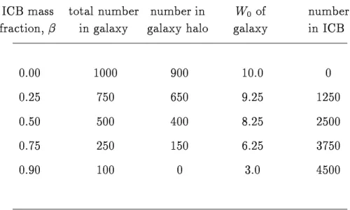
The models described here are groups of ve galaxies, with the entire group containing 5000 equal-mass particles. Group models consist of the galaxies, each represented by a number of particles, plus additional particles in a common group halo. The fraction of the total mass in this intra-cluster background (ICB) was varied from zero to 90%. To generate the initial conditions, the positions and velocities of the ICB particles and the centers of mass of the galaxies were found by randomly sampling a King (1966) distribution with W0 = 7. This ensured
that the galaxies were all bound to the group. With gravitational constant G = 1 and total mass M = 1 the group was scaled to have binding energy (ignoring the internal energy of the galaxies) E = 1=2, and to satisfy the virial theorem, K?
1
2 P
~Fi~ri = 0, where K is the total kinetic energy and ~Fi and~ri are the force
on and position of the ith particle. For the purposes of scaling each galaxy was temporarily represented by a single particle with a mass and a softening length
equal to the total mass and the 90% mass radius of the galaxy, respectively. The particles representing galaxies were then replaced with the appropriate galaxy models.
Following Barnes (1985), the galaxy models consist of a `luminous' core and a `dark' halo. The core of each galaxy contains 100 particles with the number of halo particles varying from none to 900, depending on the initial ICB mass fraction, . The total number of particles in each galaxy is thus 1000(1?), so that
the overall luminous mass fraction is always 10%. The positions and velocities of the particles are generated by sampling a King distribution; the 100 most bound particles are identied as belonging to the core with the remainder identied as halo particles. These core particles are given a softening length of one-fth that of the halo particles; which are the same as those in the ICB. The dierence in softening lengths allows the `luminous' matter in the cores to have structure on smaller scales than the more smoothly distributed `dark' halo particles. The galaxy models are scaled to obey the virial theorem and to have binding energy per unit mass Eg=Mg = 1=2; thus the internal velocity dispersions of the galaxies
roughly equal the group dispersion, as is seen in compact groups. The King central potential parameterW0 is chosen so that when the core particles are considered in
isolation their binding energy per unit mass also equals 1=2; this ensures that the cores have similar luminous mass versus radius proles for galaxies with dierently sized halos. An individual galaxy model was evolved for thirty dynamical times, and at random points after ten crossing times models were selected for use in the group model.
The distribution of particles between the galaxies and ICB is summarized in Table 4.1. In the units described above, the half-light radius of the galaxies is r1=2 = 0:009, and the 90% light radius r0:9 = 0:016; the softening length of the core
CHAPTER4. THECOMPACT GROUP MODELS 28
Table 4.1. Model Parameters for N=5000, 5 Galaxy Groups ICB mass total number number in W0 of number
fraction, in galaxy galaxy halo galaxy in ICB
0.00 1000 900 10.0 0
0.25 750 650 9.25 1250
0.50 500 400 8.25 2500
0.75 250 150 6.25 3750
particles is l= 0:008 and that of the halo particles is d = 0:04. This high degree
of softening is necessary to prevent two{body relaxation, given the relatively small number of particles in each galaxy. The core radius of the groups is 0:1 and the
half-mass radius is 0:4. Scaling the units of mass and length to M = 210 46g 10
13M
and R = 200 kpc makes the unit of time T = R=V = q
R3=GM = 0:422
Gyr; the unit of velocity is then V = 465 km/s. We use H0 = 50 km s
?1 Mpc?1
throughout this paper.
The tree code does not exactly conserve energy or momentum; with time step size t = 0:001, energy was conserved to better than 0.05% over an entire evolution, and the center of mass (originally at the origin) moved a distance of order 10?3 code units or less. A single step took roughly 120 CPU seconds on a
VAX 6420, 67 seconds on a Sun Sparcstation 2, 15 seconds on a HP 9000/730, and 2:8 seconds on a Cray Y-MP. The Cray Y-MP ran at roughly 105 Mops for these models.
3. The Evolutions
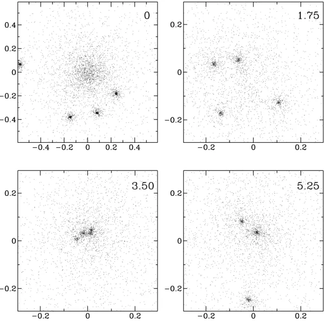
Three sets of models were constructed; for all the models in a set the galaxies initially had the same positions and velocities (to within an overall scaling factor), and within each set was varied from zero to 0.9. Each model was evolved until two galaxies were left. Figure 4.1 shows snapshots from a typical run. As a result of dynamical friction, galaxies near the center of the cluster become more tightly bound; galaxies on more extended orbits lose a considerable amount of energy when they pass near or through the core. There can be a number of close encounters and 3-body interactions before the rst merger occurs (at least for higher ). The merger product remains close to the center of the group and in time accretes the
CHAPTER4. THECOMPACT GROUP MODELS 30
Fig. 4.1.| Snapshots from a typical run with = 0:75. Note the change in scale after the rst snapshot. Times are shown in the upper right-hand corner. All of the particles are shown. The unit of length is 200 kpc and that of time is 0.422 Gyr. In the third frame there are four galaxies; the dense appearance of the group is due in part to projection eects. The central galaxy in the nal frame is the product of two mergers.
other galaxies. After accounting for the change in scale between the rst two times shown in Figure 4.1, it is still possible to see that the central density of the dark background has fallen from its initial value; this decrease is seen in the other models as well. The halo heats up as galaxies lose their orbital energy through dynamical friction, causing the background density to fall; however, the total density increases slightly over time as the galaxies move into the central region.
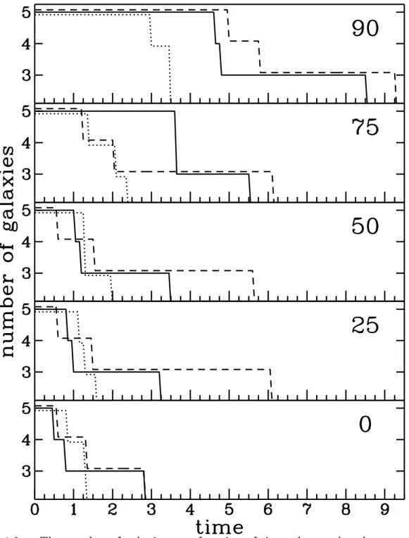
The merging histories of all the models are given in Figure 4.2, which shows the number of galaxies as a function of time for the dierent ICB mass fractions used. Galaxies are identied using the `friends-of-friends' algorithm applied to the core particles only (see Barnes 1985 for a description of this algorithm). The runs with ICB mass fraction = 0:25 and = 0:5 are not much dierent from those with all the mass attached to galaxies ( = 0); in fact, the median time of the second merger is the same for the three cases. The rst two mergers occur within 1?2 dynamical times; these mergers involve galaxies on orbits which remain close
to the core (r < 0:33). Later mergers involve galaxies on more extended orbits. The
timing of these mergers varies more, depending on the details of the initial galaxy orbits. For example, in the set of models shown by a dotted line in Figure 4.2, the third merger results in the capture of a galaxy from a highly elliptical orbit by the large remnant produced by the rst two mergers. For =0 and =0.25, this galaxy is captured on its rst pass through the center of the cluster; for larger it survives an increasing number of orbits but loses energy on each pass through the center, ultimately being captured. For comparison, the dashed line shows a set which begins with a galaxy at a similar distance from the cluster center but in a nearly circular orbit; this galaxy is also involved in the third merger, but this occurs much later than in the former set.
CHAPTER4. THECOMPACT GROUP MODELS 32
Fig. 4.2.| The number of galaxies as a function of time; the number decreases as a result of mergers. The number in the top right-hand corner of each frame gives the initial ICB mass fraction. Each line type (solid,dashed,dotted) is for models for which the same seed was used for generating the initial positions and velocities of the galaxies. Small vertical shifts were applied to the curves for clarity.
one model showing no mergers untilt = 4 but the other two showing less change. Further increasing the ICB mass fraction to = 0:9 actually delays merging by a much longer time than does increasing from 0 to 0.75; two of the = 0:9 models evolve for nearly 5 dynamical times, or 2 Gyr, before merging begins.
4. Physical Processes
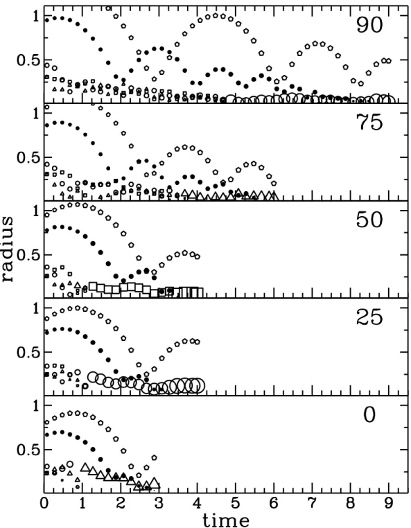
Figure 4.3 shows the radial coordinates of galaxies with respect to the center of mass as a function of time for the set of models indicated by a solid line in Figure 4.2. In the lower models, galaxies merge before signicant orbital evolution takes place. At higher , the merging cross-section is suciently reduced so that the orbits decay signicantly before the onset of merging. In all cases the product of the rst merger is involved in all later merging. The eects of dynamical friction for larger ICB mass fractions are readily apparent from Figure 4.3. Galaxies steadily sink towards the center of the group, and more elongated orbits are circularized | the apocenters are signicantly reduced while the pericenters remain nearly constant.
We can estimate the dynamical friction time scale by approximating the ICB as a singular isothermal sphere. In this case, the Chandrasekhar formula predicts that a galaxy on a circular orbit will fall to the center of the sphere in time
tfric = 1:17ln r
2
ivc
GMg (4:1)
where Mg is the mass of the galaxy, ri is the initial radius of its orbit, vc is the
circular orbit speed, and bmax=bmin is the ratio of the size of the cluster to the
size of a galaxy (Binney and Tremaine 1987, x7.1). In code units the background
extends to bmax 1:3, the velocity dispersion is roughly unity so vc p
CHAPTER4. THECOMPACT GROUP MODELS 34
Fig. 4.3.| The radial trajectories of the galaxies as a function of time for the models shown by a solid line in Figure 4.2. The size of the plotting symbol increases with the mass of the galaxy.
galaxy mass is given by Mg = (1?)=5. For = 0:9, the galaxy size bmin 0:02
and so tfric = 20r2
i; for = 0:75, bmin = 0:06 and tfric = 11r2
i.
The set of models shown by a dashed line in Figure 4.2 begins with a galaxy at r = 0:55 and low eccentricity (e 0:03). This galaxy sinks to the center and is
involved in the third merger, which occurs at t = 9:25 in the = 0:9 case and at t = 6:1 in the = 0:75 case; equation 4.1 yields times of 6.0 and 3.3, respectively. Given the approximate nature of this analysis, the agreement with the simulation results is reasonable. Note also that for 0:3 < ri < 0:5, 2 < tfric < 5 ( = 0:9); this
correlates closely with the times that merging begins and with the characteristic decay times of the trajectories shown in Figure 4.3.
In the models in this study, galaxy-galaxy interactions happen at such low relative velocities that stripping of the halos from the cores does not occur. For example, Figure 4.4 shows the number of particles bound to each galaxy as a function of time for two of the models shown in Figure 4.3. This number was found by considering each galaxy as an isolated system and determining which of the particles initially belonging to the galaxy still had negative total energy in the center-of-mass frame of that galaxy. A small amount (5-10%) of a galaxy's mass can be stripped o either as a result of galaxy-galaxy interactions (seen in galaxies near the center of the group) or of tidal interactions with the cluster background (seen in galaxies spiraling in from further out); anything more severe signies the onset of a merging event. The early stripping has little eect on the total internal energy of the galaxies. Since those particles that have gained enough energy to become unbound initially had less than average binding energy, those left behind are generally more bound.
CHAPTER4. THECOMPACT GROUP MODELS 36
Fig. 4.4.| The total number of particles bound to each galaxy for models shown in Figure 4.3: (a) 75% ICB, (b) 90% ICB. Plotting symbols for each galaxy are the same as in Figure 4.3.
galaxies is important in determining subsequent group evolution. A decrease in the geometric cross-section of the galaxies would allow a greater degree of orbital decay to take place before close encounters result in merging. Decreasing the initial mass of the galaxies would also result in longer dynamical friction timescales. The initial ratio of galaxy size to cluster size used here follows from the adoption of the condition that the velocity dispersions of the galaxies be equal to that of the group. Adopting smaller galaxy sizes would imply that the internal velocity dispersions of the galaxies would exceed that of the group, which is inconsistent with observations.
5. Group Properties
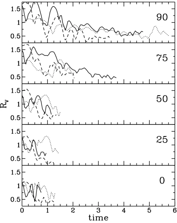
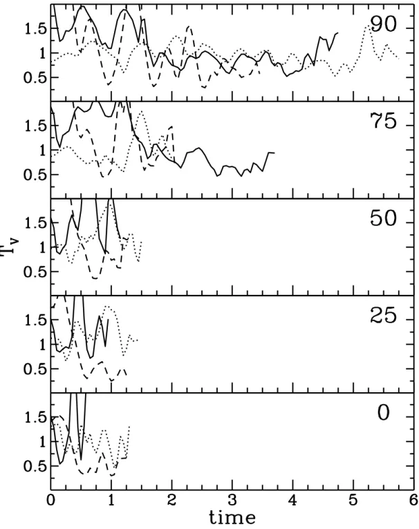
The positions, velocities, and masses of the galaxy cores found by the `friends-of-friends' algorithm were used to calculate various virial parameters of the groups as a function of time. Figure 4.5a shows the virial radius dened by
Rv = X i mi ! 2 , 0 @ X i X j<i mimj rij 1 A: (4:2)
Figure 4.5b shows the virial velocity dened by V2 v = X i miv 2 i !, X i mi ! : (4:3)
The above denitions assume that the center of mass of the group remains at the origin, which is does to a high degree of accuracy. Figure 4.5c and Figure 4.5d show the virial massM = V2
vRv and the virial crossing time T = Rv=Vv.
The initial equilibrium value of all four of these parameters is roughly unity, given the choice of units described in Section 2. The quantities Rv and Vv vary
CHAPTER4. THECOMPACT GROUP MODELS 38
Fig. 4.5.| Apparent virial quantities: (a) radius, (b) velocity, (c) mass, and (d) crossing time for all three sets of models, shown for as long as there are more than three galaxies. The linetypes are as in Figure 4.2. These quantities are calculated from the cores of the galaxies only.
CHAPTER4. THECOMPACT GROUP MODELS 40
CHAPTER4. THECOMPACT GROUP MODELS 42
models that survive longer than this, the values settle down to values in the range 0.5{0.75. The apparent crossing time shows little secular change as the groups shrink. The virial mass shows the clearest trend towards lower values, decreasing to roughly a quarter of the total mass of the system. A similar eect has been seen in earlier studies, e.g. Barnes (1985) and Mamon (1987). The discrepancy between virial and actual mass is attributable to the segregation of luminous matter to the center of the group; the virial mass is a better estimate of the mass in the volume of space which contains the luminous matter than of the total system mass. The range of values taken by the virial parameters varies little between models with diering .
Hickson and his coworkers have made photometric and spectroscopic observations of all the galaxies in his catalog of groups. (Hickson, Kindl, and Auman 1988, HMHP). They have computed the median galaxy separations, velocity dispersions, and various mass estimators for Hickson's compact groups (the HCG). For comparison with the observed values, we adopt the physical scaling of Section 2. The choice of total group mass is within the range of the masses determined by HMHP, which extend up to 210
47g, although it is larger than the
average value.
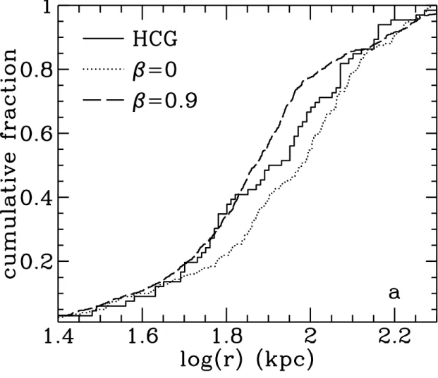
Figure 4.6a show the cumulative distribution of the median galaxy-galaxy separation for two values of . For each model, three orthogonal projections were used; the median two-dimensional separation was calculated every 0.05 time units for as long as the group contained four or more galaxies. The results for all models with the same are included the distribution. Also shown as a solid line is the distribution for Hickson's groups which contain four or more members, using the values from HMHP. Because the = 0:9 groups experience greater orbital evolution before the onset of merging, they tend to have smaller sizes than the lower
Fig. 4.6.| (a) The distribution of median two-dimensional separations for Hickson's compact groups (HCG) and for the = 0 and = 0:9 models. (b) The distribution of line-of-sight velocity dispersions. (c) The distribution of crossing times. Also shown as a dot-dash line is the distribution for = 0:9 when only those models with a maximum projected galaxy-galaxy separation of less than 180 kpc are included.
CHAPTER4. THECOMPACT GROUP MODELS 44
CHAPTER4. THECOMPACT GROUP MODELS 46
models; for intermediate the distributions are closer to the = 0 case. The median of the distribution is 74 kpc for = 0:9 and 95 kpc for = 0, compared to 85 kpc for Hickson's groups; the corresponding inter-quartile ranges are 20, 28 and 30 kpc.
The line-of-sight velocity dispersions were calculated for three orthogonal projections in the same manner as with the median separations. The values found for one dimension are multiplied by p
3 in order to compare them to the adopted three-dimensional dispersions given by HMHP. The distributions of velocities diers signicantly from the observed distribution for both values of , as is shown in Figure 4.6b. The model distributions are narrower, as would be expected given that all the models have the same total mass. Since the velocity dispersion scales as the square root of the mass, a spread in masses would increase the spread in the line-of-sight dispersions.
Figure 4.6c shows the distributions of crossing times, calculated using the estimatort = 4r=v; the factor of 4= corrects for the projection eects of using the two-dimensional median separation r, and v is p
3 times the line-of-sight velocity dispersion. The two model distributions are indistinguishable from each other, and tend towards signicantly longer crossing times than seen in Hickson's groups. The median crossing time for the models is about 26% larger than the observed value. Even if the models are rescaled to give the same median velocity as the HCG, they still have longer crossing times.
Varying has little eect on the distributions of the observable parameters of these models, particularly the crossing time. Assuming there is a spread in in the HCG, the narrowness of the observed distribution could be taken as a conrmation of this result. The fact that the observed distribution of radii is not much wider
than the model distributions is surprising, given the homogeneous nature of the models. This could indicate that the initial conditions were quite similar for all compact groups, or it may indicate that a selection eect is at work. Hickson's selection criteria were designed to pick out dense systems, and might result in the choice of groups which in projection appear to be more compact than they truly are.
HMHP nd a correlation between crossing time and spiral fraction: groups with longer crossing times have larger spiral fractions. Similarly, they nd a weak correlation between crossing time and the magnitude dierence of the rst- and second-ranked galaxies: groups with large magnitude dierences have shorter crossing times. We can look for similar relationships in our models by assuming that all the galaxies begin as spirals and that a merger results in an elliptical galaxy with a luminosity proportional to its mass. Using a Spearman rank test, no correlations with crossing time are found; this is because a merger actually increases the median separation, since a pair of galaxies with a small separation is eliminated and replaced by a single galaxy.
6. Groups of Ten Galaxies
Five evolutions of groups of 10 galaxies were run, using N=104 particles. The
same galaxy models were used; a given model has twice as many galaxies and twice as many background particles as a ve-galaxy model with the same . The initial conditions were generated in the same fashion as described in Section 2., except that a W0 = 6 King model was used to generate the ICB particle and galaxy initial
positions and velocities, making the groups less centrally concentrated; the core radii are 20 kpc. The overall scaling makes the group velocity dispersion larger
CHAPTER4. THECOMPACT GROUP MODELS 48
than the internal galaxy dispersions by a factor of p
2. These groups behaved in a manner similar to the Ng=5 groups: there is an initial merger near the center of
cluster, and the larger galaxy thus created is involved in further merging, creating a dominant central remnant.
Figure 4.7 shows the merging history of these models. As before, increasing the ICB mass fraction slows the merging rate, although the eect is less pronounced. The merging rate scales roughly with N: for = 0:75 there are six mergers in six crossing times, the same amount that it takes for the Ng=5 models to undergo
three mergers. Scaling to M = 410
46g and R = 200 kpc, such that the galaxies
have the same size and mass as for the Ng=5 models, makes the unit of velocity
V = q
GM=R = 660 km/s and that of time T = R=V = 0.30 Gyr. Thus even the = 0:9 group merged down to three galaxies in only 3 Gyr.
The virial parameters behave in a manner similar to that in theNg=5 models,
although with a lower amplitude of statistical uctuation. Again, the initial value of these parameters is unity in code units. The virial radius trends slightly lower, varying between 1 and 0.5, while the velocity dispersion drops by a factor of 2.
The virial mass decreases steadily to about one quarter of the total mass of the group. The virial crossing time uctuates around unity.
7. Summary
These models show that virialized groups of galaxies with number densities comparable to those of Hickson's groups will undergo near total merging after a small number of crossing times if the galaxies have substantial halos. The time scale for merging is longer if the dark matter in the group is smoothly distributed rather than all attached to the galaxies. With 90% of the mass in a smooth background,
Fig. 4.7.| The number of galaxies as a function of time for 10-galaxy groups. The lines are oset slightly from integer values for the sake of clarity. The ICB mass fraction is indicated in the upper right-hand corner.
CHAPTER4. THECOMPACT GROUP MODELS 50
the cluster will continue to satisfy Hickson'sN 4 criterion for roughly four times
longer than if all the mass is in galaxies. However, the time for the group to merge completely, t 4 Gyr, remains short compared with the Hubble time. Thus the
existence of these groups is still problematic even in the most extreme case explored here.
Interestingly, even though these models all have the same total mass and a rather homogeneous set of initial conditions, they still display a distribution of crossing times nearly as broad as that observed in the HCG. However, the crossing times of the HCG tend to be lower than is seen in these models.
Further discussion of these results and a comparison with other studies are given in Chapter 6.
Chapter 5
The Cluster Models
CHAPTER5. THECLUSTER MODELS 52
1. Introduction
Simulations of the dynamical interaction of galaxies in clusters have produced conicting results, as discussed in Section 3.1. This study was undertaken to reinvestigate this problem by taking advantage of the enormous increase that has occurred in available computational power during the past decade. While the simulation of a rich cluster with thousands of resolved galaxies is beyond the capacity of even a high-performance workstation, simulation of a poor cluster, such as those in the MKW (Morgan, Kayser, and White 1975) and AWM (Albert, White, and Morgan 1977) catalogs, is practical. This chapter presents poor cluster models initially containing 50 galaxies.
2. The Cluster Models
A total of ten cluster models were evolved. All of the particles in a model have identical mass; a total of N=40,000 bodies are used. The models are fully self-consistent in that each galaxy is represented as an extended structure containing many particles and the gravitational potential arises from the particles alone. Mass is apportioned between the galaxies and a smoothly distributed common group halo, or intra-cluster background (ICB). The percentage of mass initially in the ICB,, is chosen to be 50, 75, or 90. Since the total amount of mass in the cluster is the same for all models, increasing has the eect of removing mass from the galaxies and distributing it throughout the cluster. A snapshot of the initial state of a typical model is show in Figure 5.1.
To generate the initial conditions, the positions and velocities of the ICB particles and the centers of mass of the galaxies were found by randomly sampling
Fig. 5.1.| The initial conguration of a typical model. Half of the mass is in galaxies and half is in a smooth background (=50). The core radius of the cluster is 0.17 code units, or 250 kpc when scaled to a unit of length of 1.5 Mpc. The total number of particles is N = 40000.