Block Coordinate Descent for Regularized Multi-convex Optimization

Block Coordinate Descent for Regularized

Multi-convex Optimization

by

Yangyang Xu

A Thesis Submitted

in Partial Fulfillment of the

Requirements for the Degree

Master of Arts

Approved, Thesis Committee:

Wotao Yin, Chair

Associate Professor of Computational and Applied Mathematics

Richard Tapia University Professor

Maxfield-Oshman Professor in Engineering

Computational and Applied Mathematics

Yin Zhang

Professor of Computational and Applied Mathematics

Richard Baraniuk

Victor E. Cameron Professor of Electrical and Computer Engineering

Houston, Texas

November, 2012

Block Coordinate Descent for Regularized Multi-convex Optimization

by

Yangyang Xu

This thesis considers regularized block multi-convex optimization, where the fea-sible set and objective function are generally non-convex but convex in each block of variables. I review some of its interesting examples and propose a generalized block coordinate descent (BCD) method. The generalized BCD uses three differ-ent block-update schemes. Based on the property of one block subproblem, one can freely choose one of the three schemes to update the corresponding block of variables. Appropriate choices of block-update schemes can often speed up the algorithm and greatly save computing time. Under certain conditions, I show that any limit point satisfies the Nash equilibrium conditions. Furthermore, I establish its global conver-gence and estimate its asymptotic converconver-gence rate by assuming a property based on the Kurdyka- Lojasiewicz inequality. As a consequence, this thesis gives a global linear convergence result of cyclic block coordinate descent for strongly convex opti-mization. The proposed algorithms are adapted for factorizing nonnegative matrices and tensors, as well as completing them from their incomplete observations. The al-gorithms were tested on synthetic data, hyperspectral data, as well as image sets from the CBCL, ORL and Swimmer databases. Compared to the existing state-of-the-art algorithms, the proposed algorithms demonstrate superior performance in both speed and solution quality.

First, I want to express my deepest appreciation to my advisor, Professor Wotao Yin, who is my committee chair. He continuously and convincingly conveys to me a spirit of research and gradually leads me to the exciting academic research way. With-out his guidance, precious advice and persistent encouragement, this thesis would not be possible.

Secondly, I would like to thank my committee members, Professor Richard Tapia, Professor Yin Zhang, and Professor Richard Baraniuk. They spend a lot of precious time reviewing my thesis and make great advice, which are very helpful to improve the overall quality of my thesis.

In addition, I want to thank Professor Zaiwen Wen, who carefully and patiently helped me solve some critical issues encountered during my research. Also, I want to thank the staff in our department. They provide generous help to my research.

Finally, I would like to particularly thank my lovely wife, Jun. She accompanies me, encourages me, and gives me the best care. She helps me in both of my everyday and academic life. Without her persistent help and encouragement, it is impossible to conquer every difficulty and make every achievement.

Abstract ii

Acknowledgments iii

List of Illustrations vii

1 Introduction

1

1.1 Problem description . . . 5

1.2 Motivation by applications . . . 6

1.2.1 Blind source separation . . . 7

1.2.2 Nonnegative matrix factorization . . . 8

1.2.3 Low-rank matrix recovery . . . 9

1.2.4 Nonnegative tensor factorization . . . 9

1.3 Method description . . . 10

1.3.1 Block coordinate descent with different block updates . . . 11

1.3.2 Why use different block updates . . . 13

1.4 Overview of existing results . . . 14

1.4.1 Block minimization scheme . . . 14

1.4.2 Block proximal scheme . . . 16

1.4.3 Block prox-linear scheme . . . 17

1.5 Contributions . . . 17

1.6 Organization . . . 18

2 Convergence analysis

19

2.3 Kurdyka- Lojasiewicz inequality . . . 31

2.4 Global convergence and rate . . . 35

3 Nonnegative tensor factorization and completion

39

3.2 An algorithm for nonnegative tensor factorization . . . 42

3.3 Convergence results . . . 44

3.4 An algorithm for nonnegative tensor completion . . . 46

4 Numerical results

48

4.1.1 Overview of some algorithms . . . 49

4.1.2 Parameter setting . . . 51

4.1.3 Synthetic data . . . 52

4.1.4 Image data . . . 53

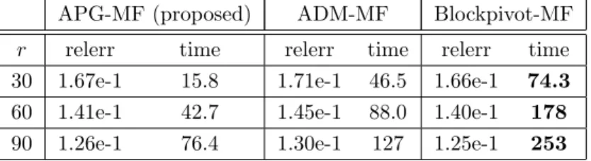
4.1.5 Hyperspectral data . . . 56

4.2 Nonnegative matrix completion . . . 58

4.3 Nonnegative three-way tensor factorization . . . 59

4.3.1 Synthetic data . . . 61

4.3.2 Image test . . . 61

4.3.3 Hyperspectral data . . . 63

4.4 Nonnegative tensor completion . . . 66

4.5 Summary . . . 70

5 Conclusions

71

A Some proofs

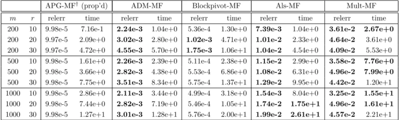
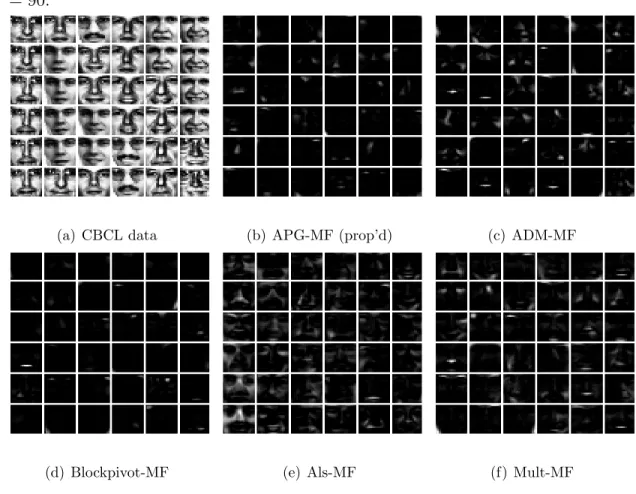
72

4.1 How extrapolation improves the algorithm . . . 50 4.2 One trial on nonnegative matrix factorization with m= 500, q= 30 . 54 4.3 CBCL database and base images: (a) 36 images selected from the

2000 tested images; (b)-(f) 36 base images corresponding to the first 36 columns of A1 obtained by APG-MF (prop’d), ADM-MF,

Blockpivot-MF, Als-MF and Mult-MF at r= 90. . . 55 4.4 ORL database and base images: (a) 50 images selected from 400

tested images; (b)-(d) 50 base images corresponding to the first 50 columns ofA1 obtained from APG-MF, ADM-MF and

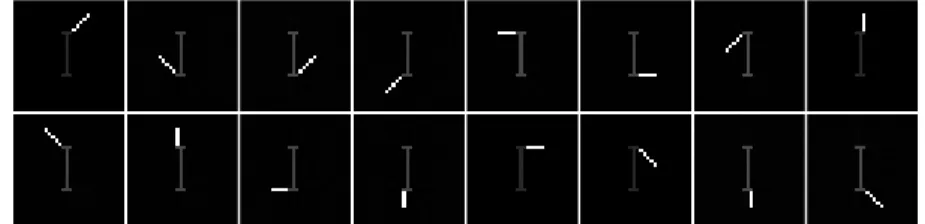
Blockpivot-MF at r= 90. . . 57 4.5 Hyperspectral data of 150×150×163: four selected slices are shown 58 4.6 16 selected images in Swimmer dataset . . . 62 4.7 Factor images obtained by doing NMF on Swimmer database; r= 16

is set in (4.1) . . . 62 4.8 Factor images obtained by doing NTF on Swimmer database;r = 60

is set in (4.5). The “limb” parts are obtained by superimposing the

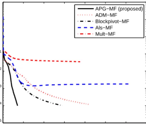
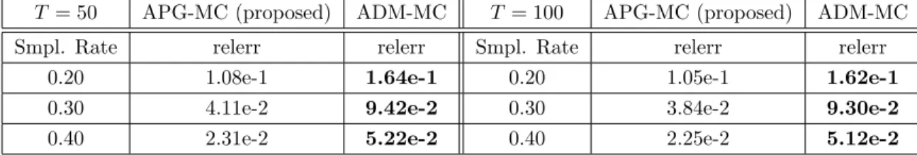
corresponding rank-1 factors of NTF. . . 62 4.9 Relative error versus running time (in seconds) for 8 independent

Chapter 1

Introduction

One type of optimization problem that arises in many applications has the following two properties: (i) its objective can be written as a sum of a smooth function and a (non-smooth) separable function; (ii) its variables can be partitioned into a few disjoint blocks, and the objective can be jointly non-convex but convex with respect to each block of variables while all the others are fixed. One particular example is dictionary learning with `1-regularizer [60]

min D,Θ 1 2kDΘ−Xk 2 F +λkΘk1, subject to D∈ D, (1.1)

whereD={D:kdjk ≤1, j = 1, . . . , K}is used to control the scale ofD,dj denotes

the jth column ofD and kΘk1 = P

i,j|θij|. Using indicator function

δD(D) =        0 if D ∈ D ∞ otherwise one can write (1.1) as

min D,Θ 1 2kDΘ−Xk 2 F +λkΘk1+δD(D), (1.2)

whose objective is a sum of the smooth term 1₂kDΘ−Xk2

F and non-smooth separable

two blocks: D and Θ. The objective is jointly non-convex since the product DΘ

couplesD and Θtogether. However, it is convex with respect to each one of the two blocks while the other is fixed.

For some of these problems, computing the gradient of the objective over all variables can be very expensive such as the tensor decomposition [44]

min A1,···,AN 1 2kM−A1◦A2◦ · · · ◦ANk 2 F, (1.3)

or even impossible due to the existence of non-smooth terms such as in (1.1). There-fore, direct gradient descent is not a suitable choice to solve these problems. Tra-ditional second-order methods such as interior point method or Newton’s method are not good choices either due to non-smoothness. One popular and often efficient method for solving these problems is the alternating minimization method, which al-ternatively updates each block of variables by minimizing the objective with respect to one block at a time while all the others are fixed. For example, it is applied in [18] to tensor decomposition (1.3) by cyclically updating the factor matrices A1,· · · ,AN

via Ak_n = argmin An 1 2kM−A k 1 ◦ · · · ◦A k n−1◦An◦Akn−1+1◦ · · · ◦A k−1 N k 2 F,∀n. (1.4)

Each subproblem in (1.4) can be written into a convex quadratic programming by the property of tensor-matrix multiplication (see Section 3.1) and has a closed form solution. Alternating minimization has also been applied in [72] to group Lasso regularized problem (see (1.8) below), [88] to low-rank matrix recovery (see (1.12) below), and [33] to nonnegative matrix factorization (see (1.11) below).

Alternating minimization is favorable for these problems because it is usually difficult to update all variables simultaneously but relatively easy to update one block at a time. This method can be generalized to block coordinate descent (BCD) method, which also updates the variables block by block. Unlike its name would indicate, BCD does not have to decrease the objective during the update of each block. It is really a method by block-coordinate update. There are flexible ways to carry out the block update, by minimizing either the original objective or a relaxed version of the objective with respect to one block at a time with all others fixed. For some applications, minimizing a relaxed problem at each iteration can make overall better performance than minimizing the original one. For example, it was observed in [62] that alternating minimization (1.4) for tensor decomposition may cause a so-called swamp effect, which means the convergence rate dramatically slows down within exceedingly high number of iterations. However, the swamp effect can be reduced if the objective plus a proximal term is minimized at each iteration, namely,

Ak_n= argmin An 1 2kM−A k 1◦ · · · ◦An◦ · · · ◦AkN−1k 2 F + µk 2 kAn−A k−1 n k 2 F,∀n. (1.5)

Each subproblem in (1.5) can also be written as a convex quadratic programming and has a closed form solution. In addition, for some applications, it may be difficult to solve block subproblems. For example, if we consider nonnegative tensor decom-position, namely, nonnegativity is enforced in (1.3), then both (1.4) and (1.5) with additional constraints An ≥0 are not easy to solve. However, it will become easy if

the first term in (1.5) is locally linearized, namely, Ak_n = argmin An≥0 hGk_n,An−Akni+ µk 2 kAn−A k−1 n k 2 F,∀n, (1.6) where Gk

n is the partial gradient about An of the first term in (1.5) at Akn. Each

subproblem in (1.6) has a closed form solution. This kind of block-update scheme is new and can be more efficient than alternating minimization as shown later in this thesis for nonnegative tensor decomposition.

BCD has been applied to both convex and non-convex problems. It is relatively easy to establish global convergence for BCD applied to convex smooth optimization. For non-convex smooth problems, only subsequence convergence results have been established for special cases such as [58] considering quadratic functions and [30] assuming strict quasiconvexity of each block subproblem. The global convergence of BCD for non-convex optimization is still an open problem. Non-smoothness also makes it difficult to establish the convergence of BCD even for convex problems (see the review in Section 1.4). This thesis will give a global convergence result of BCD for a special class of non-convex optimization problems which may have non-smooth terms in the objective.

The rest of this chapter first gives a mathematical description of the considered problem and then overviews some interesting examples which arise in applications. These examples are the motivation of my work in this thesis. After that, BCD is for-mally described, and the existing results of BCD are overviewed. Global convergence analysis and practical performance of BCD will be given in subsequent chapters.

1.1

Problem description

Before describing the problem, let me give a key related definition.

Definition 1.1 (Block multi-convexity)

A setX ⊂_Rn _{is called block multi-convexunder the partition: x= (x}

1,· · · ,xs)∈ X

if the projection of X to each block of components is convex, namely, for each i and fixed(s−1) blocks x1,· · · ,xi−1,xi+1,· · · ,xs, the set

Xi(x1,· · · ,xi−1,xi+1,· · · ,xs),{xi ∈Rni : (x1,· · · ,xi−1,xi,xi+1,· · · ,xs)∈ X }

is convex. A function f(x)is called block multi-convexif for each i,f(x) is a convex function of xi while all the other blocks are fixed.

In this thesis, I consider the regularized multiconvex optimization problem

min x∈X F(x1,· · · ,xs)≡f(x1,· · · ,xs) + s X i=1 ri(xi), (1.7)

where variablexis decomposed intos disjoint blocksx1,· · ·,xs, the setX of feasible

points is assumed to be a closed and block multi-convex subset of _Rn_{, f is assumed}

to be a differentiable and block multi-convex function, and regularization terms ri,

i= 1,· · · , s, are extended-valued convex functions. The set X and functionf can be non-convex over x= (x1,· · · ,xs). However, when all but one blocks are fixed, (1.7)

over the free block is a convex problem.

Extended valued means ri(xi) is valued on R ∪ {∞}. In particular, ri (or a

part of it) can be an indicator function of convex sets, so ri can include individual

individual constraints ofx1,· · · ,xs, respectively, when they are present. In addition,

ri can include non-smooth functions such as`1-norm kxik1 and `2-norm kxik, which

often give some structures on the solution.

1.2

Motivation by applications

A large number of practical problems can be formulated in the form of (1.7) includ-ing both convex and non-convex problems. One convex example arisinclud-ing in signal processing is the basis pursuit (denoising) [19] or more generally, sparse group Lasso [80, 91] min x 1 2kAx−bk 2_+λ 1 s X i=1 kxik+λ2kxk1, (1.8)

where x has been partitioned into s disjoint blocks: x = (x1, . . . ,xs). Another

example arising in machine learning is the multi-class logistic regression [27, 12]

min W − 1 n n X i=1 " _m X j=1 yij(w>j xi)−log m X j=1 exp(w>_j xi) !# +λkWk2 F,

where yij = 1 if data point xi belongs to class j and yij = 0 otherwise, and wj is the

jth column of W.

There are also many non-convex examples such as sparse dictionary learning (1.1) and the ones overviewed below. The work in this thesis is timely and mainly motivated by these non-convex problems.

1.2.1 Blind source separation

Let s1, . . . ,sn ∈ R1×p be a set of source signals. Given m sensor signals xi =

Pn

j=1aijsj +ηi, i = 1,· · · , m, where A = [aij]m×n ∈ Rm×n is an unknown mixing

matrix and η_i is noise, blind source separation (BSS) [36] aims to estimate both A

and S = [s>₁, . . . ,s>_n]>. It has found applications in many areas such as artifact re-moval [35] and image processing [37]. Two classical approaches for BSS are principle component analysis (PCA) [78] and independent component analysis (ICA) [22]. If

m < n and no prior information on A and S is given, these methods will fail. As-sumings1,· · · ,sn are sparse under some dictionary B∈RT×p, namely,si =yiB and

yi ∈R1×T is sparse fori= 1, . . . , n, [96, 15] use the sparse BSS model

min A,Y λ 2kAYB−Xk 2 F +r(Y), subject to A∈ D (1.9)

where Y = [y>₁,· · ·,y>_n]> ∈ _Rn×T_{, r(Y) is a sparsity regularizer such as r(Y) =}

kYk1, D is a convex set to control the scale of A such as kAkF ≤ 1, and λ is

a balancing parameter. Note that model (1.9) is block multi-convex in A and Y

each but jointly non-convex. The block constraint A ∈ D can be included into the objective by adding the indicator functionδD(A). A similar model appears in cosmic

microwave background analysis [13] which solves

min A,Y λ 2trace (AYB−X) > C−1(AYB−X)+r(Y), subject toA ∈ D (1.10)

for a certain covariance matrixC. Algorithms for (sparse) BSS include online learning algorithm [1], feature extraction method [52], feature sign algorithm [49], and so on.

1.2.2 Nonnegative matrix factorization

Nonnegative matrix factorization (NMF) was first proposed by Paatero and his cowork-ers in the area of environmental science [67]. The later popularity of NMF can be partially attributed to the publication of [47] in Nature. It has been widely applied in data mining such as text mining [69] and image mining [50], dimension reduction and clustering [20, 89], hyperspectral endmember extraction, as well as spectral data analysis [68]. A widely used model for (regularized) NMF is

min X,Y 1 2kXY−Mk 2 F +r1(X) +r2(Y), subject to X∈Rm+×r,Y ∈Rr ×n + (1.11) where M ∈ _Rm×n

+ is the input nonnegative matrix, r1, r2 are some regularizers

pro-moting solution structures, and

Rm+×n,{A∈R

m×n _:a

ij ≥0,∀i, j}.

The block constraintsX∈_Rm×r

+ andY ∈Rr ×n

+ can be respectively incorporated into

the regularization termsr1 andr2 using ˆr1 =r1+δ_Rm×r

+ and ˆr2 =r2+δR

r×n

+ . The new

regularizers ˆr1 and ˆr2 both include block constraint and another (non-smooth) term.

Two early popular algorithms for NMF are the projected alternating least squares method [67] and multiplicative updating method [48]. Due to the bi-convexity (multi-convexity under two-block partition) of the objective in (1.11), a series of alternating nonnegative least square (ANLS) methods (alternating minimization) have been pro-posed such as in [51, 39, 41] to solve (1.11). Recently, the classic alternating direction method (ADM) [29, 28] has been applied in [95] to (1.11).

1.2.3 Low-rank matrix recovery

Similar models of (1.11) also arise in low-rank matrix recovery, such as the one con-sidered in [73] min X,Y 1 2kA(XY)−bk 2_+αkXk2 F +βkYk 2 F, (1.12)

whereA is a linear operator. A particularly interesting case is the matrix completion problem, where A is the sampling operator PΩ defined by

(PΩ(Z))ij =        zij, if (i, j)∈Ω, 0, otherwise.

A special application of this problem is the famous Netflix problem, which aims to complete users’ ratings to all movies from their highly incomplete ratings. Methods for solving (1.12) include augmented Lagrangian method [73], stochastic gradient method [74], and nonlinear succesive over-relaxation (SOR) method [88].

1.2.4 Nonnegative tensor factorization

Nonnegative tensor factorization (NTF) is a generalization of NMF to multi-way arrays. It has been applied in a variety of areas including computer vision [79], hyperspectral analysis [94] and feature selection [9]. One commonly used model for NTF is based on CANDECOMP/PARAFAC tensor decomposition [87]

min A1,···,AN≥0 1 2kM−A1◦A2◦ · · · ◦ANk 2 F + N X n=1 rn(An); (1.13)

and another one is based on Tucker decomposition [43] min G,A1,···,AN≥0 1 2kM−G ×1A1×2A2· · · ×N ANk 2 F +r(G) + N X n=1 rn(An), (1.14)

where M is a given nonnegative tensor, r, r1,· · · , rN are regularizers, and “◦” and

“×n” represent outer product and tensor-matrix multiplication, respectively. The

necessary background of tensor will be reviewed in Chapter 3. Using a similar ap-proach as in Section 1.2.2, one can incorporate each block constraint Ai ≥0 into its

corresponding regularization term ri.

Most algorithms for solving NMF have been directly extended to NTF. For exam-ple, the multiplicative update in [67] is extended to solving (1.13) in [79]. The ANLS methods in [39, 41] are extended to solving (1.13) in [40, 42]. Algorithms for solving (1.14) include the column-wise coordinate descent method [53] and the alternating least square method [26]. More about NTF algorithms can be found in [93].

1.3

Method description

For convex optimization, we have a rich set of tools, which own both nice numerical performance and theoretical results. However, very few works have established strong theoretical guarantees for non-convex optimization. Though the methods mentioned in last section are practically efficient for solving the overviewed non-convex examples, to the best of my knowledge, none of them have been shown to globally converge. This motivates me to make an efficient algorithm with global convergence for solving problems in the form of (1.7).

1.3.1 Block coordinate descent with different block updates

Generally, it is difficult to update all the blocks of variables in (1.7) simultaneously but usually easy to do so block by block. My main interest is theblock coordinate descent

(BCD) method of the Gauss-Seidel type, which minimizesF or its relaxation cyclically over each ofx1,· · · ,xs while fixing the remaining blocks at their last updated values.

Letxk

i denote the value of xi after its kth update, and

f_ik(xi),f(xk1,· · · ,x

k

i−1,xi,xki+1−1,· · · ,x

k−1

s ), for all i and k. (1.15)

Within each cycle, for i= 1, . . . , s,xi is updated by one of the next three schemes

Block minimization: xk_i = argmin xi∈Xik

f_ik(xi) +ri(xi), (1.16a)

Block proximal: xk_i = argmin xi∈Xik f_ik(xi) + Lk_i−1 2 kxi−x k−1 i k 2_+r i(xi), (1.16b)

Block prox-linear: xk_i = argmin xi∈Xik hˆgk_i,xi−xˆki−1i+ Lk_i−1 2 kxi−xˆ k−1 i k 2_+r i(xi), (1.16c) whereLk_i−1 >0 is some parameter,Xk

i ,Xi(xk1,· · · ,xki−1,xk −1

i+1,· · · ,xk −1

s ) and in the

last type of update (1.16c),

ˆ

xk_i−1 =xk_i−1+ω_ik−1(xk_i−1−xk_i−2) (1.17) denotes an extrapolated point,ω_ik−1 ≥0 is the extrapolation weight, ˆgk_i =∇f_ik(ˆxk_i−1) is the block-partial gradient of f at ˆxk_i−1. I consider extrapolation (1.17) for update (1.16c) since it can significantly accelerate the convergence of BCD in the applica-tions; see numerical results in Chapter 4. However, the extrapolation can make the

whole objective increasing and cause numerical instability. Hence, the kth itera-tion is repeated one time with ω_ik−1 = 0 for all blocks updated by (1.16c) whenever

F(xk_)≥F(xk−1_{). As long asx}k_6=xk−1_{, the algorithm makesF(x}k_{)< F(x}k−1_{). The}

framework of BCD is given in Algorithm 1.

Algorithm 1Block coordinate descent method for solving (1.7)

Initialization: choose initial points (x−1₁ ,· · ·,x−1_s ) = (x0₁,· · · ,x0_s) for k= 1,2,· · · do

fori= 1,2,· · ·, s do xk

i ←(1.16a), (1.16b), or (1.16c).

end for

if stopping criterion is satisfied then return (xk₁,· · ·,xk_s).

end if

if F(xk)≥F(xk−1) then

Re-update xk with ωk_i−1 = 0 for every blockiupdated by (1.16c). end if

end for

Since X and f are block multi-convex, all three subproblems in (1.16) are convex. In general, the three updates generate different sequences and can thus cause BCD to converge to different solutions. I found in many tests, applying (1.16c) on all or some blocks gives solutions of lower objective values, for a possible reason that its local prox-linear approximation helps avoid the small regions around certain local minima. In addition, it is generally more time consuming to compute (1.16a) and (1.16b) than (1.16c) though each time the former two tend to make larger objective decreases than applying (1.16c) without extrapolation.

(1.16b). For instance, if ri = δDi the indicator function of convex set Di (equivalent toxi ∈ Di), (1.16c) reduces to xk_i =P_Xk i∩Di xˆ k−1 i −gˆ k−1 i /L k−1 i , (1.18) whereP_Xk

i∩Di is the project to set X

k i ∩ Di. Ifri(xi) =λikxik1 andXik=Rni, (1.16c) reduces to xk_i =S_Lk−1 i /λi xˆ k−1 i −gˆ k−1 i /L k−1 i , (1.19)

where Sν(·) is soft-thresholding defined component-wise as Sν(t) = sign(t) max(|t| −

ν,0). More examples arise in joint/group `1 and nuclear norm minimization, total

variation, etc.

1.3.2 Why use different block updates

I consider all of the three updates since they fit different applications, and also differ-ent blocks in the same application, yet their convergence can be analyzed in a unified framework. For example, it may be better to apply BCD with (1.16a) to low-rank ma-trix recovery (1.12), whereas BCD with (1.16c) can be more suitable for nonnegative matrix factorization (1.11). For sparse dictionary learning (1.1), (1.16a) or (1.16b) may be better for D-subproblem, while (1.16c) seems better for Θ-subproblem.

To ensure the convergence of Algorithm 1, for every block i to which (1.16a) is applied, I will require fk

i (xi) to be strongly convex, and for every block i to which

(1.16c) is applied, I will require ∇fk

i (xi) to be Lipschitz continuous. The parameter

convergence, it is allowed to change during the iterations. Use of (1.16b) only requires

Lk

i to be uniformly lower bounded from zero and uniformly upper bounded. In fact,

fk

i in (1.16b) can be nonconvex, and my proofs still go through. (1.16b) is a good

replacement of (1.16a) if f_ik is not strongly convex. Use of (1.16c) requires more conditions on Lk

i; see Lemmas 2.2 and 2.3. (1.16c) is relatively easy to solve and

often allows closed form solutions such as in the cases of (1.18) and (1.19). For block

i, (1.16c) is prefered over (1.16a) and (1.16b) when the latter two are expensive to solve and fk

i has Lipschitz continuous gradient. Overall, the three choices cover a

large number of cases.

1.4

Overview of existing results

In the literature of BCD, the first two block-update schemes in (1.16) have been widely used and extensively studied, and the third one (1.16c) is quite new and has been used in some very recent works for solving convex problems.

1.4.1 Block minimization scheme

Block minimization (1.16a) is the most-used form in the literature of BCD and has been extensively studied. BCD with block minimization is exactly the alternating minimization method. It is closely related to the Gauss-Seidel or SOR methods in [66] for solving equation systems. It has a long history dating back to 1950s [32], which considers strongly concave quadratic programming. Convergence of

alternat-ing minimization typically requires F to be convex (or pseudoconvex or hemivariate) differentiable and have bounded level sets [86, 92, 4, 70]. With these nice properties, alternating minimization was shown to make the objective converge to optimal value. If F is further assumed to be strictly convex, the iterates themselves will converge to the unique solution [57]. When F is non-convex, alternating minimization may cycle and stagnate [71]. However, subsequence convergence can be obtained for spe-cial cases such as quadratic function [58], strict quasi-convexity in each of the first (s−2) blocks [30], unique minimizer per block [56]. If F is non-differentiable, al-ternating minimization can get stuck at a non-stationary point even if F is convex; see p.94 of [4]. Hence, alternating minimization was generally regarded unsuitable for non-smooth optimization. Nevertheless, if the non-differentiable part is separable such as in the form of (1.7), subsequence convergence can still be obtained for some special cases. The first work considering such a separable nonsmooth structure is by Auslender in [4] which assumes strong convexity of F. In [31], a decomposition method was proposed for minimizing a strictly convex quadratic function over the intersection of convex sets, and it turns out to be alternating minimization for a dual functional of a convex problem in the form of (1.7) as shown in [81]. The work [82] established subsequence convergence result of BCD for non-convex non-smooth prob-lem by assuming separable structure of the non-smooth part and pseudoconvexity of the smooth part. However, global convergence is still unknown for non-convex non-smooth optimization even if the non-smooth part is separable.

1.4.2 Block proximal scheme

Block proximal update (1.16b) can be regarded as alternatively applying one step of the proximal point method to block subproblems. The proximal point method has been extensively studied, and it is usually related to the maximal monotone operator; see [76, 25] and references therein. It has also been used with BCD, and the first work appears to be [5] which applied BCD with block proximal update to convex problems in the form of (1.7). For two-block convex programs, [11] proposed a partial proximal method which iteratively updates both blocks simultaneously by minimizing the objective plus a proximal term involving only one block. The work [30] has extended the method to smooth non-convex optimization with block separable constraints, and it shows that every limit point of the iterates is a critical point. Using the proximal term L

k−1

i

2 kxi−x

k−1

i k2 in (1.16b) can often stabilize the iterates as shown

in [62] which applied BCD with block proximal update to tensor decomposition and demonstrated that it could reduce a so-called swamp effect. Recently, this method was revisited in [3] for non-convex problems with two blocks and separable non-smooth part, and it was shown that the iterates globally converge to a limit point via the Kurdyka- Lojasiewicz (KL) inequality, whose definition will be given in Chapter 2. However, the global convergence for over-two block non-convex optimization is still unknown.

1.4.3 Block prox-linear scheme

Block prox-linear update (1.16c) with extrapolation is new in the literature of BCD but very similar to the update in the block-coordinate gradient descent (BGD) method of [84], which identifies a block descent direction by gradient projection and then per-forms an Armijo-type line search. [84] does not use extrapolation (1.17). It considers more general f that is smooth but not necessarily multi-convex, but it does not consider joint constraints. For convex smooth optimization, Nesterov [65] recently proposed a randomized BCD, which randomly selects a block of variables and uses prox-linear method to update the selected block at each step. Meanwhile, he obtained a sublinear convergence of the randomized BCD for convex problems with Lipschitz continuous gradient and linear convergence for strongly convex problems. His work has been extended to convex non-smooth optimization in [75], which obtained sim-ilar convergence rate results. However, the convergence rate of cyclic BCD is still unknown, even for strongly convex optimization. In addition, none has applied BCD with block prox-linear update to non-convex optimization. This thesis will also give global convergence of this method and show its high efficiency on nonnegative tensor factorization and completion.

1.5

Contributions

Motivated by many practical problems, I characterize and formulate them into reg-ularized multiconvex optimization. To solve this kind of problem, I choose block

coordinate descent (BCD) method due to its simplicity and efficiency. Also, I gen-eralize BCD by incorporating three different block-update schemes. In addition, I establish global convergence and asymptotic convergence rate in a unified way for BCD with all the three block-update schemes. Then, the algorithm with prox-linear update (1.16c) is applied to two classes of problems (i) nonnegative matrix/tensor

factorization and (ii) nonnegative matrix/tensor completion from incomplete obser-vations, and is demonstrated superior than the state-of-the-art algorithms on both synthetic and real data in both speed and solution quality.

1.6

Organization

The rest of the thesis is organized as follows. Chapter 2 first gives a subsequence convergence result of Algorithm 1. Then it briefly overviews the Kurdyka- Lojasiewicz inequality through which a global convergence result is given. In Chapter 3, tensor is overviewed, and then Algorithm 1 is applied to both the nonnegative matrix/tensor

factorization problem and the completion problem. Numerical results are presented in Chapter 4. Finally, Chapter 5 concludes the thesis.

Chapter 2

Convergence analysis

This chapter will first give some key definitions and then analyze the convergence of Algorithm 1. The convergence analysis takes two steps. Under certain assump-tions, the first step establishes the square summable result P

kkx

k _−xk+1_k2 _{< ∞}

and obtains subsequence convergence to Nash points (see Definition 2.6), as well as global convergence to a single Nash point under a fairly strong condition: the se-quence of iterates is bounded and the Nash points are isolated. The second step presents a different approach for global convergence; specifically, it assumes the KL inequality [16, 17] and improves the result to P

kkxk−xk+1k <∞, which gives the

algorithm global convergence, as well as asymptotic rates of convergence. The classes of functions that obey the KL inequality are reviewed.

2.1

Elements of analysis

Before starting the analysis, let me give some key definitions which can be found in [77, 83]. Throughout the analysis, I use the vector productha,bi=a>b=Pn

i=1aibi

for a,b ∈_Rn _{and Euclidean norm kak=}p

ha,ai.

Definition 2.1 (Feasible direction)

there is τ >0such that x+td∈ X for any t∈[0, τ).

Definition 2.2 (Effective domain)

The effective domain of a function f on _Rn _{is dom(f) ={x∈}

Rn:f(x)<+∞}. Definition 2.3 (Limiting Fr´echet subdifferential)

A vector g∈_Rn _{is a Fr´echet subgradient of continuous function f atx∈dom(f)if}

lim inf y→x,y6=x

f(y)−f(x)− hg,y−xi ky−xk ≥0.

The set of Fr´echet subgradient off atxis called Fr´echet subdifferential and denoted as ∂fˆ (x). If x6∈dom(f), then ∂f(x) =∅.

The limiting Fr´echet subdifferential is denoted by∂f(x) and defined as

∂f(x) = {g ∈_Rn_{: there isx}

n→x and gn ∈∂fˆ (xn) such that gn→g}.

When f is differentiable at x, ∂f(x) = ˆ∂f(x) = {∇f(x)}. For convex function f,

∂f(x) = ˆ∂f(x) and is the set of all vectors gx satisfying

f(y)≥f(x) +hgx,y−xi, ∀y∈dom(f).

For problem (1.7), it is shown in [3] that

∂F(x) ={∇x1f(x) +∂r1(x1)} × · · · × {∇xsf(x) +∂rs(xs)}, where D1× D2 denotes the Cartesian product of D1 and D2 defined by

Definition 2.4 (Strong convexity)

A function f is said to be strongly convex with modulus µ > 0 if for any x,y ∈ dom(f), f(y)≥f(x) +hgx,y−xi+ µ 2ky−xk 2 , for all gx ∈∂f(x). (2.1)

If µ= 0 in (2.1), then f is weakly convex or, commonly called, convex. In addition, if µ= 0 and the inequality holds strictly,f is called strictly convex.

Definition 2.5 (Directional derivative)

Forx∈dom(f), the (lower) directional derivative f0(x;d)along the direction d is

f0(x;d) = lim inf

t↓0

f(x+td)−f(x)

t .

If f is differentiable atx, then f0(x;d) = ∇f(x)>d.

Definition 2.6 (Nash point)

Given a feasible setX, a pointx= (x1, . . . ,xs)∈dom(f)∩ X is called a Nash point

or block coordinate-wise minimizer if the Nash equilibrium conditions

f(x)≤f(x+ (0, . . . ,0,di,0, . . . ,0)), i= 1, . . . , s (2.2)

hold for any feasible direction (0, . . . ,0,di,0, . . . ,0) atx.

When f is block multi-convex, (2.2) is equivalent to

f0(x; (0, . . . ,0,di,0, . . . ,0))≥0, i= 1, . . . , s. (2.3)

According to the definition, a point ¯x is a Nash point of (1.7) if for i= 1,· · · , s,

or equivalently

h∇xif(¯x) + ¯pi,xi−¯xii ≥0, for all xi ∈X¯i and for some ¯pi ∈∂ri(¯xi), (2.5) where ¯Xi =Xi(¯x1,· · ·,x¯i−1,x¯i+1,· · · ,x¯s).

Definition 2.7 (Critical point)

Given a feasible set X, a point x∈dom(f)∩ X is called a critical point or stationary point if f0(x;d)≥0 for any feasible direction d∈_Rn _{at x.}

Ifx is an interior point ofX, thenxsatisfies (2.3) if and only if x is a critical point, and in this case, it holds0∈∂f(x). A special case isX =_Rn_.

Definition 2.8 (Difference measure of two sets)

The difference of two sets X,Y is measured by

diff(X,Y) = max

sup x∈X

inf

y∈Ykx−yk, _ysup_∈Yxinf∈Xkx−yk

.

If limn→∞diff(Xn,X) = 0, then there is xn ∈ Xn such that limn→∞kxn−xk= 0.

Throughout the analysis, I make the following assumptions.

Assumption 2.1

In (1.7), F is continuous in dom(F) and infx∈dom(F)F(x)>−∞. Problem (1.7) has

a Nash point.

Assumption 2.2

Each blockiis updated by the same scheme among(1.16a)–(1.16c)for allk. LetI1,I2

and I3 denote the set of blocks updated by (1.16a), (1.16b)and (1.16c), respectively.

1. for i ∈ I1, fik defined in (1.15) is strongly convex of xi with modulus `i ≤

Lk_i−1 ≤Li;

2. for i∈ I2, parameters Lki−1 obey `i ≤Lki−1 ≤Li;

3. for i∈ I3, ∇fik is Lipschitz continuous and parameters L k−1 i obey `i ≤Lki−1 ≤ Li and f_ik(xk_i)≤f_ik(ˆxk_i−1) +hˆgk_i,xk_i −xˆk_i−1i+ L k−1 i 2 kx k i −xˆ k−1 i k 2_{. (2.6)} Remark 2.1

The same notation Lk_i−1 is used in all three schemes for the simplicity of unified convergence analysis, but I want to emphasize that it has different meanings in the three different schemes. For i∈ I1, Lki−1 is not a parameter subject to user selection

but a property constant that is determined by the objective and the current values of all other blocks, while for i ∈ I2 ∪ I3, Lki−1 is subject to user selection and must

meet certain conditions to guarantee convergence. For i ∈ I2, Lki−1 can be simply

fixed to a positive constant or selected by a pre-determined rule to be uniformly lower bounded from zero and upper bounded. For i∈ I3, Lki−1 is selected to satisfy (2.6).

Taking Lk_i−1 as the Lipschitz constant of ∇fk

i can satisfy (2.6). However, it allows

smaller Lk_i−1, which can speed up the algorithm.

Remark 2.2

In addition, I want to emphasize that I make different assumptions on the three different schemes. The use of (1.16a) requires block strong convexity with modulus uniformly away from zero and upper bounded, and the use of (1.16c)requires block

Lipschitz continuous gradient. The use of (1.16b) requires neither strong convexity nor Lipschitz continuity. Even the block convexity is unnecessary for (1.16b), and the proof still goes through. Each assumption on the corresponding scheme guarantees sufficient decrease of the objective and makes square summable; see Lemma 2.2, which plays the key role in the convergence analysis.

2.2

Subsequence convergence

The analysis in this subsection follows the following steps. First, I show sufficient descent at each step (inequality (2.12) below), from which I establish the square summable result (Lemma 2.2 below). Next, the square summable result is exploited to show that any limit point is a Nash point in Theorem 2.1 below. Finally, with the additional assumptions of isolated Nash points and bounded{xk_{}, global convergence}

is obtained in Theorem 2.2 below. The first step is essential while the last two steps use rather standard arguments. I begin with the following lemma similar to Lemma 2.3 of [8]. Since the proof in [8] does not consider constraints, I include a slightly changed proof for completeness.

Lemma 2.1

Let ξ1(u) and ξ2(u) be two convex functions defined on the convex set U and ξ1(u)

be differentiable. Let ξ(u) = ξ1(u) +ξ2(u)and

u∗ = argmin u∈U h∇ξ1(v),u−vi+ L 2ku−vk 2 +ξ2(u). (2.7)

If ξ1(u∗)≤ξ1(v) +h∇ξ1(v),u∗−vi+ L 2ku ∗₋ vk2_{, (2.8)} then ξ(u)−ξ(u∗)≥ L 2ku ∗₋ vk2_+Lhv−u,u∗₋ vi for any u ∈ U. (2.9)

Proof. The first-order optimality condition of (2.7) holds

h∇ξ1(v) +L(u∗−v) +g,u−u∗i ≥0, for any u∈ U, (2.10)

for some g∈∂ξ2(u∗). For any u ∈ U, we have

ξ(u)−ξ(u∗)≥ξ(u)− ξ1(v) +h∇ξ1(v),u∗−vi+ L 2ku ∗_−vk2 −ξ2(u∗) =ξ1(u)−ξ1(v)− h∇ξ1(v),u−vi+h∇ξ1(v),u−u∗i+ξ2(u) −ξ2(u∗)− L 2ku ∗₋ vk2 ≥ξ2(u)−ξ2(u∗)− hg,u−u∗i −Lhu∗−v,u−u∗i − L 2ku ∗₋ vk2 ≥ −Lhu∗−v,u−u∗i −L 2ku ∗₋ vk2 =L 2ku ∗₋ vk2_+Lhv−u,u∗₋ vi,

where the first inequality uses (2.8), the second inequality is obtained from the con-vexity of ξ1 and (2.10), and the last inequality uses the convexity of ξ2 and the fact

g∈∂ξ2(u∗). This completes the proof.

Based on this lemma, I can show the key lemma below.

Lemma 2.2 (Square summable kxk_−xk+1_k)

with 0≤ωk_i−1 ≤δω

r

Lk_i−2

Lk_i−1 for 0< δω <1uniformly over all i∈ I3 and k. Then

∞ X

k=0

kxk−xk+1k2 <∞. (2.11)

Proof. For i ∈ I3, we have the inequality (2.6) by Item 3 of Assumption 2.2. Let

F_ik _, f_ik+ri and take ξ1 = fik, ξ2 = ri,v = ˆxki−1 and u = x k−1

i in (2.9). All the

conditions required by Lemma 2.1 are satisfied. Hence, we have

F_ik(xk_i−1)−F_ik(xk_i)≥ L k−1 i 2 kˆx k−1 i −x k ik 2_+Lk−1 i hˆx k−1 i −x k−1 i ,x k i −xˆ k−1 i i = L k−1 i 2 kx k−1 i −x k ik2− Lk_i−1 2 (ω k−1 i ) 2_kxk−2 i −x k−1 i k 2 _(2.12) ≥ L k−1 i 2 kx k−1 i −x k ik 2₋ L k−2 i 2 δ 2 ωkx k−2 i −x k−1 i k 2 . (2.13)

Fori∈ I1∪I2, we haveFik(x k−1

i )−Fik(xki)≥ Lk_i−1

2 kx

k−1

i −xkik2,which can be obtained

by the strong convexity of F_ik(xi) for i ∈ I1 or the update (1.16b) for i ∈ I2, and

thus the inequality (2.13) still holds. Therefore,

F(xk−1)−F(xk) = s X i=1 F_ik(xk_i−1)−F_ik(xk_i) ≥ s X i=1 Lk_i−1 2 kx k−1 i −x k ik 2₋L k−2 i δω2 2 kx k−2 i −x k−1 i k 2 .

Summing the above inequality over k from 1 toK, we have

F(x0)−F(xK)≥ K X k=1 s X i=1 Lk_i−1 2 kx k−1 i −x k ik 2₋ L k−2 i 2 δ 2 ωkx k−2 i −x k−1 i k 2 ≥ K X k=1 s X i=1 (1−δ2 ω)L k−1 i 2 kx k−1 i −x k ik 2 _≥ K X k=1 (1−δ2 ω)` 2 kx k−1_−xk_k2_,

where ` = mini`i > 0. Since 0 < δω < 1 and F is lower bounded, taking K → ∞

Remark 2.3

From the proof above, we can see that Algorithm 1 makes F(xk)> F(xk+1) as long as xk 6=xk+1.

Now, I can establish the following subsequence convergence result.

Theorem 2.1 (Limit point is Nash point)

Under the assumptions of Lemma 2.2 and further assuming the set mapXi(·)

contin-uously changes in X, namely, xk0_{,x∈ X and x}k0 _→ximply

lim k→∞diff Xi(xk 0 1 , . . . ,x k0 i−1,xk 0 i+1, . . . ,x k0 s ),Xi(x1, . . . ,xi−1,xi+1, . . . ,xs) = 0, ∀i,

then any limit pointx¯of{xk}is a Nash point, namely, satisfying the Nash equilibrium conditions (2.4) or (2.5).

Proof. Let ¯x be a limit point of {xk_{} and {x}kj} _{be the subsequence converging} to ¯x. The closedness of X implies ¯x ∈ X. Since {Lk_i} is bounded, passing another subsequence if necessary, we haveLkj

i converges to some ¯Li fori= 1,· · · , sasj → ∞.

Inequality (2.11) implies that kxk+1_−xk_{k →0, so {x}kj+1} _{also converges to ¯x.} For i∈ I1, we have Fkj+1 i (x kj+1 i )≤F kj+1 i (xi), ∀xi ∈ X kj+1 i . (2.14)

Letting j → ∞, we can show (2.4) by the continuity of F and the set map Xi(·).

Suppose otherwise for some block i0 ∈ I1, there is yi0 ∈X¯i0 such that

Since limjdiff Xkj+1 i0 , ¯ Xi0 = 0, there is yj_i 0 ∈ X kj+1

i0 such that limjy

j

i0 =yi0. From

the continuity of F, we have

lim j→∞F(x kj+1 1 , . . . ,x kj+1 i0−1,y j i0,x kj i0+1, . . . ,x kj s ) = F(¯x1,· · · ,x¯i0−1,yi0,x¯i0+1,· · ·,x¯s). (2.16) Note that (2.14) implies

F(xkj+1 1 , . . . ,x kj+1 i0−1,x kj+1 i0 ,x kj i0+1, . . . ,x kj s )≤F(x kj+1 1 , . . . ,x kj+1 i0−1,y j i0,x kj i0+1, . . . ,x kj s ).

Letting j → ∞ and using (2.16), we get

F(¯x1,· · · ,x¯i0−1,x¯i0,x¯i0+1,· · · ,¯xs)≤F(¯x1,· · · ,¯xi0−1,yi0,x¯i0+1,· · · ,x¯s),

which contradicts to (2.15). Hence, (2.4) holds. Similarly, for i∈ I2, we have for any xi ∈X¯i

F(¯x1,· · · ,x¯i−1,x¯i,x¯i+1,· · · ,x¯s)≤F(¯x1,· · · ,x¯i−1,xi,x¯i+1,· · · ,x¯s) + ¯ Li 2 kxi−x¯ik 2_, namely, ¯ xi = argmin xi∈X¯i F(¯x1,· · · ,x¯i−1,xi,x¯i+1,· · · ,x¯s) + ¯ Li 2 kxi−x¯ik 2_{. (2.17)}

Thus, ¯xi satisfies the first-order optimality condition of (2.17), which is precisely

(2.5). For i∈ I3, we have xkj+1 i = argmin xi∈Xkj +1 i h∇fkj+1 i (ˆx kj i ),xi−ˆx kj i i+ Lkj i 2 kxi−xˆ kj i k 2_+r i(xi).

The convex proximal minimization is continuous in the sense that the output xkj+1

i

depends continuously on the input ˆxkj

i [76]. Letting j → ∞, from x kj+1 i → x¯i and ˆ xkj i →x¯i, we get ¯ xi = argmin xi∈X¯i h∇xif(¯x),xi−x¯ii+ ¯ Li 2 kxi−x¯ik 2 +ri(xi). (2.18)

Hence, ¯xi satisfies the first-order optimality condition of (2.18), which is precisely

(2.5). This completes the proof.

Remark 2.4

The continuity ofXi(·)holds if X is convex; see Theorem 4.32 in [77]. A special case

is X =_Rn_{, in which case we can immediately have the following corollary.}

Corollary 2.1

LetX =_Rn_{in(1.7). Under the assumptions of Lemma 2.2, any limit pointx¯ of{x}k_}

is a critical point of (1.7), namely, 0∈∂F(¯x).

Theorem 2.2 (Global convergence given isolated Nash points)

Let N be the set of Nash points of (1.7). Under the assumptions of Lemma 2.2, we have dist(xk_{,N)→0, if {x}k_{} is bounded. Further, if N contains uniformly isolated}

points, namely, there isη >0such thatkx−yk ≥ηfor any distinct pointsx,y∈ N, then xk _{converges to a point in N.}

Moreover, if F is strictly convex and X = _Rn_{, then x}k _{converges to the unique}

solution of (1.7).

Proof. Suppose dist(xk_{,N) does not converge to 0. Then there exists ε > 0 and a}

{xkj_{}implies that it must have a limit point ¯x∈ N according to Theorem 2.1, which} is a contradiction.

From dist(xk_{,N) → 0, it follows that there is an integer K}

1 > 0 such that xk ∈ ∪y∈NB(y,η₃) for all k ≥ K1, where B(y,η₃) , {x ∈ X : kx−yk < η₃}. In

addition, Lemma 2.2 implies that there exists another integer K2 > 0 such that

kxk_−xk+1_{k <} η

3 for all k ≥ K2. Take K = max(K1, K2) and assume x

K _{∈ B(¯x,}η

3)

for some ¯x ∈ N. We claim that for any ¯x 6= y ∈ N, kxk−yk > η₃ holds for all

k ≥K. This claim can be shown by induction onk ≥K. If somexk _∈B(¯x,η

3), then kxk+1−x¯k ≤ kxk+1−xkk+kxk−x¯k< 2η 3 , and kxk+1−yk ≥ k¯x−yk − kxk+1−x¯k> η 3, for any ¯x6=y∈ N. Therefore, xk _{∈ B(¯x,}η

3) for all k ≥ K since x

k _{∈ ∪}

y∈NB(y,η₃), and thus {xk} has

the unique limit point ¯x, which meansxk _→x¯.

When F is strictly convex and X = _Rn, there is only one critical point, which is the unique solution. Hence, xk _{converges to the unique solution.}

Remark 2.5

The boundedness of {xk} is guaranteed if the level set {x ∈ X : F(x) ≤ F(x0)} is bounded. However, the isolation assumption does not hold, or holds but is difficult to verify, for many functions. This motivates another approach below for global convergence.

2.3

Kurdyka- Lojasiewicz inequality

Before proceeding with the analysis, let me briefly review the Kurdyka- Lojasiewicz inequality, which is central to the global convergence analysis in the next subsection.

Definition 2.9 (Kurdyka- Lojasiewicz property)

A functionψ(x)satisfies the Kurdyka- Lojasiewicz (KL) property at pointx¯ ∈dom(∂ψ) if there existsθ ∈[0,1)such that

|ψ(x)−ψ(¯x)|θ

dist(0, ∂ψ(x)) (2.19)

is bounded around x¯ under the notational conventions: 00 _{= 1,∞/∞ = 0/0 = 0. In}

other words, in a certain neighborhood U of x¯, there exists φ(s) = cs1−θ for some c >0 and θ ∈[0,1) such that the KL inequality holds

φ0(|ψ(x)−ψ(¯x)|)dist(0, ∂ψ(x))≥1,∀x∈ U ∩dom(∂ψ) and ψ(x)6=ψ(¯x), (2.20)

where dom(∂ψ)_,{x:∂ψ(x)6=∅} and dist(0, ∂ψ(x))_,min{kyk:y∈∂ψ(x)}. This property was introduced by Lojasiewicz [55] on real analytic functions, for which the term with θ∈[1₂,1) in (2.19) is bounded around any critical point ¯x. Kur-dyka extended this property to functions on theo-minimal structure in [45]. Recently, the KL inequality was extended to nonsmooth sub-analytic functions [16]. Since it is not trivial to check the conditions in the definition, I give some examples below that satisfy the KL inequality.

Real analytic functions

A smooth function ϕ(t) on _R is analytic if

ϕ(k)_(t)

k! 1_k

is bounded for all k and on any compact set D ⊂ _R. One can verify whether a real function ψ(x) on _Rn _is

analytic by checking the analyticity of ϕ(t) _, ψ(x+ty) for any x,y ∈ _Rn_{. For}

example, any polynomial function is real analytic such as kAx−bk2 _{and the first}

terms in the objectives of (1.13) and (1.14). In addition, it is not difficult to verify that the non-convex function Pn

i=1(x 2 i +ε2)q/2+ 1 2λkAx−bk 2 _{with 0 < q < 1 and}

ε >0 considered in [46] for sparse vector recovery is a real analytic function (the first term is the ε-smoothed `q semi-norm). The logistic loss function log(1 +e−t) is also

analytic. Therefore, all the above functions satisfy the KL property with θ ∈ [1₂,1) in (2.19).

Locally strongly convex functions

A function ψ(x) is strongly convex in a neighborhood D with modulusµ > 0 if

ψ(y)≥ψ(x) +hγ(x),y−xi+µ

2kx−yk

2_{, for all γ(x)∈∂ψ(x) and for anyx,y∈ D.}

According to the definition and using the Cauchy-Schwarz inequality, we have

ψ(y)−ψ(x)≥ hγ(x),y−xi+µ 2kx−yk 2 _{≥ −}1 µkγ(x)k 2 , for all γ(x)∈∂ψ(x).

Hence, µ(ψ(x)−ψ(y))≤dist(0, ∂ψ(x))2_{, and ψ satisfies the KL inequality (2.20) at}

any point y ∈ D with φ(s) = _µ2√s and U = D ∩ {x : ψ(x) ≥ ψ(y)}. For example, the logistic loss function log(1 +e−t) is strongly convex in any bounded set D, so it

has the KL property with θ= 1₂.

Semi-algebraic functions

A setD ⊂ _Rn _{is calledsemi-algebraic [14] if it can be represented as}

D= s [ i=1 t \ j=1 {x∈_Rn_:p ij(x) = 0, qij(x)>0},

where pij, qij are real polynomial functions for 1 ≤ i ≤ s, 1 ≤ j ≤ t. A function

ψ is called semi-algebraic if its graph Gr(ψ) _, {(x, ψ(x)) : x ∈ dom(ψ)} is a semi-algebraic set.

Semi-algebraic functions are sub-analytic, so they satisfy the KL inequality accord-ing to [16, 17]. I list some elementary properties of semi-algebraic sets and functions below as they help identify semi-algebraic functions.

1. If a set D is semi-algebraic, so is its closure cl(D).

2. If D1 and D2 are both semi-algebraic, so are D1∪ D2,D1∩ D2 and Rn\D1.

3. Indicator functions of semi-algebraic sets are semi-algebraic.

4. Finite sums and products of semi-algebraic functions are semi-algebraic.

5. The composition of semi-algebraic functions is semi-algebraic.

From items 1 and 2, any polyhedral set is semi-algebraic such as the nonnegative orthant _Rn

+ = {x ∈ Rn : xi ≥ 0,∀i}. Hence, the indicator function δRn+ is a

its graph is cl(D), where

D ={(t, s) :t+s= 0,−t >0} ∪ {(t, s) :t−s= 0, t >0}.

Hence, the `1-norm kxk1 is semi-algebraic since it is the finite sum of absolute

func-tions. In addition, the sup-norm kxk∞ is semi-algebraic, which can be shown by

observing Graph(kxk∞) = {(x, t) :t = max j |xj|}= [ i {(x, t) :|xi|=t,|xj| ≤t,∀j 6=i}.

Further, the Euclidean norm kxkis shown to be semi-algebraic in [14]. According to item 5, kAx−bk1,kAx−bk∞ and kAx−bkare all semi-algebraic functions.

Sum of real analytic and semi-algebraic functions

Both real analytic and semi-algebraic functions are sub-analytic. According to [14], if ψ1 and ψ2 are both sub-analytic andψ1 maps bounded sets to bounded sets, then

ψ1+ψ2 is also sub-analytic. Since real analytic functions map bounded set to bounded

set, the sum of a real analytic function and a semi-algebraic function is sub-analytic, so the sum satisfies the KL property. For example, the sparse logistic regression function ψ(x, b) = 1 n n X i=1 log 1 + exp −ci(a>i x+b) +λkxk1

2.4

Global convergence and rate

If {xk} is bounded, then Theorem 2.1 guarantees that there exists one subsequence converging to a Nash point of (1.7). In this subsection, I assume X = _Rn _and

strengthen this result for problems with F obeying the KL inequality. Recall that any Nash point is a critical point whenX =_Rn. The analysis here was motivated by [3], which applies the inequality to establish the global convergence of the alternating proximal point method — the special case of BCD with two blocks and using update (1.16b).

In the sequel, I use the notationFk =F(xk) and ¯F =F(¯x). First, let me establish

the following pre-convergence result, the proof of which is given in the Appendix.

Lemma 2.3 (Pre-convergence)

Under Assumptions 2.1 and 2.2, let {xk_{}be the sequence generated by Algorithm 1.}

Assume 1. Lk_i ≥`k−1 = mini∈I3L k−1 i and ωik≤δω q `k−1 Lk i

, δω <1, for all i∈ I3 and k;

2. ∇f is Lipschitz continuous on any bounded set;

3. F satisfies the KL inequality at x¯, namely, there exists φ(s) = cs1−θ _{for some}

c >0 and θ ∈[0,1)such that within some neighborhood U of x¯, it holds

φ0(|F(x)−F(¯x)|)dist(0, ∂F(x))≥1,∀x∈ U ∩dom(∂F)and F(x)6=F(¯x); (2.21)

Then there exists someB ⊂ U ∩dom(∂F) such that{xk} ⊂ B and xk converges to a point in B.

Remark 2.6

In the lemma, the required closeness of x0 to x¯ depends on U, φ and F; see the inequality in(A.1). The extrapolation weight ωk

i must be smaller than it is in Lemma

2.2 in order to guarantee sufficient decrease at each iteration.

The following corollary is a straightforward application of Lemma 2.3.

Corollary 2.2 (Local convergence to global minimizer)

Under the assumptions of Lemma 2.3, {xk_{} converges to a global minimizer of (1.7)}

if the initial point x0 is sufficiently close to any global minimizerx¯.

Proof. Suppose F(xk0_{) =F(¯x) at some k}

0. Then xk =xk0 for allk ≥ k0, according

to Remark 2.3. Now consider F(xk_{) > F(¯x) for all k ≥ 0, and thus Lemma 2.3}

implies that xk converges to some critical point x∗ if x0 is sufficiently close to ¯x, where x0_,x∗_{,x¯ ∈ B. If F(x}∗_{) > F(¯x), then the KL inequality (2.21) indicates}

φ0(F(x∗)−F(¯x)) dist (0, ∂F(x∗))≥1,which is impossible since 0∈∂F(x∗). Next, I give the global convergence result of Algorithm 1.

Theorem 2.3 (Global convergence)

Under the assumptions of Lemma 2.3 and that {xk_{} has a finite limit point x¯ where}

F satisfies the KL inequality (2.21), the sequence {xk} converges to x¯, which is a critical point of (1.7).

F(xk0_{) = F(¯x) at some k}

0, then xk = xk0 = ¯x for all k ≥ k0 from Remark 2.3.

It remains to consider F(xk_{) > F(¯x) for all k ≥ 0. Since ¯x is a limit point and}

F(xk_{)→F(¯x), there must exist an integer k}

0 such that xk0 is sufficiently close to ¯x

as required in Lemma 2.3 (see the inequality in (A.1)). The conclusion now directly

follows from Lemma 2.3.

I can also estimate the asymptotic rate of convergence, and the proof is given in the Appendix.

Theorem 2.4 (Convergence rate)

Assume the assumptions of Lemma 2.3, and suppose that xk _{converges to a critical}

point x¯, at which F satisfies the KL inequality (2.21) with φ(s) = cs1−θ _{for c > 0}

and θ ∈[0,1). Then

1. If θ = 0,xk converges to ¯xin finite iterations; 2. If θ ∈(0,1₂], kxk_{−x¯k ≤Cτ}k_{, ∀k≥k} 0, for certain k0 >0, C >0, τ ∈[0,1); 3. If θ ∈(1 2,1), kx k_{−x¯k ≤Ck}−(1−θ)/(2θ−1)_{, ∀k ≥k} 0, for certain k0 >0, C >0.

When F is strongly convex, global linear convergence can be obtained. The result is summarized in the next theorem.

Theorem 2.5 (Global linear convergence for strongly convex optimization)

Under Assumptions 2.1 and 2.2, let {xk}be the sequence generated by Algorithm 1. Let `k _{= min}

i∈I3L

k

i, and choose Lki ≥ `k−1 and ωki ≤ δω

q

`k−1

Lk i

, δω <1, for all i ∈ I3

and k. If F is strongly convex, then xk _{globally linearly converges to the unique}

Proof. When F is strongly convex, it has the KL property (2.19) with θ = 1₂ atx∗. Hence, item 2 in Theorem 2.4 holds. In addition, note that the neighborhood U in (2.20) is the whole space asF is strongly convex, sok0 = 0 in item 2. This completes

Chapter 3

Nonnegative tensor factorization and completion

In this section, I apply Algorithm 1 to the factorization and completion of nonnegative matrices and tensors. Since a matrix is a two-way tensor, I present the algorithm for tensors. I will first overview tensor and its two popular factorizations and then describe in details how to apply Algorithm 1 to nonnegative tensor factorization and its completion. Global convergence results are obtained directly from the analysis in Chapter 2.

3.1

Overview of tensor

A tensor is a multi-dimensional array. For example, a vector is a first-order tensor, and a matrix is a second-order tensor. The order of a tensor is the number of dimensions, also called way ormode. For an N-waytensor X ∈_RI1×I2×···×IN_{, denote} its (i1, i2,· · · , iN)th element by xi1i2···iN. Below I list some concepts related to tensor. For more details about tensor, the reader is referred to the review paper [44].

1. fiber: afiber of a tensorX is a vector obtained by fixing all indices ofX except one. For example, a row of a matrix is a mode-2 fiber (the 1st index is fixed), and a column is a mode-1 fiber (the 2nd index is fixed). I use xi1···in−1:in+1···iN

to denote a mode-n fiber of an Nth-order tensor X.

2. slice: a slice of a tensor X is a matrix obtained by fixing all indices of X

except two. Take a third-order tensorX for example. Xi::,X:j:, andX::kdenote

horizontal, lateral, and frontal slices ofX, respectively.

3. matricization: the mode-n matricization of a tensor X is a matrix whose columns are the mode-n fibers of X in the lexicographical order. Let X(n)

denote the mode-n matricization of X.

4. tensor-matrix product: the mode-n product of a tensor X ∈ _RI1×I2×···×IN with a matrix A∈_RJ×In _{is a tensor of sizeI}

1× · · ·In−1 ×J ×In+1× · · · ×IN defined as (X ×nA)i1···in−1jin+1···iN = In X in=1 xi1i2···iNajin. (3.1) In addition, let me briefly review the matrix Kronecker, Khatri-Rao and Hadamard products below, which are used to derive tensor-related computations.

The Kronecker product of matricesA ∈_Rm×n_{andB ∈}

Rp×qis an mp×nq matrix defined by A⊗B=             a11B a12B · · · a1nB a21B a22B · · · a2nB .. . ... . .. ... am1B am2B · · · amnB             .

The Khatri-Rao product of matrices A∈_Rm×q _{and B ∈}

Rp×q is an mp×q matrix: AB = [a1⊗b1, a2⊗b2, · · · , aq⊗bq],

whereai,bi are the ith columns of A andB, respectively. TheHadamard product of

matrices A,B ∈_Rm×n _{is the componentwise product defined by}

A∗B =             a11b11 a12b12 · · · a1nb1n a21b21 a22b22 · · · a2nb2n .. . ... . .. ... am1bm1 am2bm2 · · · amnbmn             .

Two important tensor decompositions are the CANDECOMP/PARAFAC (CP) [38] and Tucker [85] decompositions. The former one decomposes a tensor X ∈

RI1×I2×···×IN _{in the form of}X _=A

1◦A2◦ · · · ◦AN,whereAn ∈RIn×r, n= 1,· · · , N

are factor matrices, r is the tensor rank of X, and the outer product “◦” is defined as xi1i2···iN = r X j=1 a(1)_i 1ja (2) i2j· · ·a (N) iNj, for in∈[In], n= 1,· · · , N,

where a(_ijn) is the (i, j)th element of An and [I] , {1,2,· · · , I}. The latter Tucker

decomposition decomposes a tensorX in the form ofX =G×1A1×2A2· · · ×NAN,

where G ∈_RJ1×J2×···×JN _{is called the core tensor and A}

n ∈RIn×Jn, n = 1,· · · , N are

3.2

An algorithm for nonnegative tensor factorization

One can obtain a nonnegative CP decomposition of a nonnegative tensor M ∈

RI1×···×IN _{by solving} min1

2kM−A1◦A2◦ · · · ◦ANk

2

F, subject to An ∈R+In×r, n = 1,· · · , N (3.2)

where r is a specified order and the Frobenius norm of a tensor X ∈ _RI1×···×IN _is defined as kXkF = s X i1,i2,···,iN x2 i1i2···iN.

Similar models based on the CP decomposition can be found in [40, 23, 42]. One can obtain a nonnegative Tucker decomposition of M by solving

min1 2kM−G×1A1×2A2· · · ×NANk 2 F, subject toG ∈R J1×···×JN + ,An ∈RI+n×Jn,∀n, (3.3) as in [43, 61, 53]. Usually, it is computationally expensive to updateG. Since applying Algorithm 1 to problem (3.3) involves lots of computing details, I focus on applying it with block-update (1.16c) to problem (3.2).

Let A= (A1,· · · ,AN) and F(A) = F(A1,A2,· · · ,AN) = 1 2kM−A1◦A2◦ · · · ◦ANk 2 F

be the objective of (3.2). Consider updatingAn at iteration k. Using the fact that if

X =A1◦A2◦ · · · ◦AN, thenX(n) =An(AN · · ·An+1An−1· · ·A1) > , we have F(A) = 1 2 M(n)−An(AN · · ·An+1An−1· · ·A1) > 2 F ,

and ∇AnF = An(AN · · ·An+1An−1· · ·A1) > −M(n) (AN · · ·An+1An−1· · ·A1). Let Bk_n−1 =Ak_N−1 · · ·A_nk−1₊₁Ak_n−1· · ·Ak₁. (3.4) Take Lk_n−1 = max(`k−2,k(Bk<sub>n</sub>−1)>B<sub>n</sub>k−1k), where `k−2 = minnLkn−2 and kAk is the

spectral norm of A. Let

ωk_n−1 = min ωˆk−1, δω s `k−2 Lk−1 n ! (3.5)

whereδω <1 is pre-selected and ˆωk−1 = tk−_t1−1

k witht0 = 1 andtk= 1 2 1 +q1 + 4t2 k−1 . In addition, let ˆ A_nk−1 =Ak_n−1+ω_nk−1(Ak_n−1 −Ak_n−2) and ˆ Gk_n−1 = ˆ Ak_n−1(Bk_n−1)>−M(n) Bk_n−1 (3.6)

be the gradient. Then we derive the update (1.16c):

Ak_n= argmin An≥0 D ˆ Gk_n−1,An−Aˆkn−1 E +L k−1 n 2 An− ˆ Ak_n−1 2 F ,

which can be written in the closed form

Ak_n= max0,Aˆk_n−1−Gˆk_n−1/Lk_n−1. (3.7) At the end of iterationk, check whether F Ak

≥F Ak−1

. If so, re-updateAk n by

Remark 3.1

In (3.7), Gˆk_n−1 is most expensive to compute. To efficiently compute it, write ˆ

Gk_n−1 = ˆAk_n−1(Bk_n−1)>Bk_n−1−M(n)Bkn−1

Using the fact

(AB)>(AB) = (A>A)∗(B>B)

we can compute (Bk_n−1)>Bk_n−1 by

(Bk_n−1)>Bk_n−1 = (Ak₁)>Ak₁∗· · ·∗ (Ak_n−1)>A_nk₋₁∗ (Ak_n−1₊₁)>Ak_n−1₊₁∗· · ·∗ (Ak_N−1)>Ak_N−1. Then, M(n)Bkn−1 can be obtained by the so-called

matricized-tensor-times-Khatri-Rao-product [7].

Algorithm 2 summarizes how to apply Algorithm 1 with block-update (1.16c) to problem (3.2).

3.3

Convergence results

Since problem (3.2) is a special case of problem (1.7), the convergence results in Chapter 2 apply to Algorithm 2. LetDn =RI+n×randδDn(·) be the indicator function onDn forn = 1,· · · , N. Then (3.2) is equivalent to

min A1,···,AN Q(A)≡F(A) + N X n=1 δDn(An). (3.8)

According to the discussion in Section 2.3,Qis a semi-algebraic function and satisfies the KL property (2.19) at any feasible point. Further, we get θ 6= 0 in (2.19) for Q