A Supervised Learning Algorithm for Learning
Precise Timing of Multiple Spikes in Multilayer
Spiking Neural Networks
Aboozar Taherkhani , Member, IEEE, Ammar Belatreche, Member, IEEE, Yuhua Li, Senior Member, IEEE,
and Liam P. Maguire, Member, IEEE
Abstract— There is a biological evidence to prove information is coded through precise timing of spikes in the brain. However, training a population of spiking neurons in a multilayer network to fire at multiple precise times remains a challenging task. Delay learning and the effect of a delay on weight learning in a spiking neural network (SNN) have not been investigated thoroughly. This paper proposes a novel biologically plausible supervised learning algorithm for learning precisely timed multiple spikes in a multilayer SNNs. Based on the spike-timing-dependent plasticity learning rule, the proposed learning method trains an SNN through the synergy between weight and delay learning. The weights of the hidden and output neurons are adjusted in parallel. The proposed learning method captures the contri-bution of synaptic delays to the learning of synaptic weights. Interaction between different layers of the network is realized through biofeedback signals sent by the output neurons. The trained SNN is used for the classification of spatiotemporal input patterns. The proposed learning method also trains the spiking network not to fire spikes at undesired times which contribute to misclassification. Experimental evaluation on benchmark data sets from the UCI machine learning repository shows that the proposed method has comparable results with classical rate-based methods such as deep belief network and the autoencoder models. Moreover, the proposed method can achieve higher classification accuracies than single layer and a similar multilayer SNN.
Index Terms— Multilayer neural network, spiking neural network (SNN), supervised learning, synaptic delay.
I. INTRODUCTION
S
PIKE-timing-dependent plasticity (STDP) plays a prominent role in learning biological neurons, and it represents one form of synaptic plasticity which underpinsManuscript received April 4, 2017; revised October 27, 2017 and January 11, 2018; accepted January 16, 2018. This work was supported by the Ulster University’s Vice Chancellor’s Research Scholarship Scheme. (Corresponding author: Aboozar Taherkhani.)
A. Taherkhani is with the Computational Neuroscience and Cognitive Robotics Laboratory, Nottingham Trent University, Nottingham NG1 4FQ, U.K. (e-mail: [email protected]).
A. Belatreche is with the Department of Computer and Information Sciences, Northumbria University, Newcastle upon Tyne NE1 8ST, U.K. (e-mail: [email protected]).
Y. Li is with the School of Computer Science and Informatics, Cardiff University, Cardiff CF10 3AT, U.K. (e-mail: [email protected]).
L. P. Maguire is with the Faculty of Computing and Engineering, Ulster University, Londonderry BT48 7JL, U.K. (e-mail: [email protected]).
Color versions of one or more of the figures in this paper are available online at http://ieeexplore.ieee.org.
Digital Object Identifier 10.1109/TNNLS.2018.2797801
synaptic weight changes based on the precise times of pre and postsynaptic spikes [1]. STDP highlights the important role of precise spike times in information processing in the brain [2]. In addition, the rapid sensory processing observed in the visual, auditory, and olfactory systems supports the assumption that information is encoded in the precise timing of the spikes [3]–[5]. Moreover, using precise timing of spikes results in a higher information encoding capacity compared with rate-based coding [6], and it can also convey the information related to rate of spikes in a multispike coding scheme [2]. Furthermore, as neural activity is metabolically expensive, the high number of spikes involved in rate coding scheme demands a significant amount of energy and resources [7], [8]. Despite the existing evidence supporting information encoding using the precise timing of spikes, the exact neuronal mechanisms that underlie learning to fire at precise times are still not clear and remain as one of the challenging problems in the field of spiking neural networks (SNNs) [2], [9]–[11].
In this paper, a novel supervised learning algorithm inspired by STDP is proposed to train an SNN to fire multiple spikes at precise desired times. Local synaptic biochemical events, produced by incoming spikes, are used to adjust weights and delays appropriately. In addition, neurons in the output and hidden layers interact with each other through a biofeedback signal sent by the output neurons to train the network. The main novelty of the proposed method consists in: 1) capturing the effect of synaptic delays on the learning of neuronal connection weights in an SNN, which has not been consid-ered in previous works and 2) learning the spiking network synaptic delays. In addition, the proposed approach introduces an additional training mechanism to prevent the occurrence of undesired spikes which contribute to the misclassification of spatiotemporal input patterns. The proposed approach is validated using benchmark classification data sets and is compared against both spiking and rate-based neural models including state-of-the-art deep learning and autoencoder mod-els. The experimental results show an improvement in learning accuracy over existing competitive SNN architectures and comparable performance to state-of-the-art rate-based neural models.
The remainder of this paper is structured as follows. A brief review of background and related work on SNNs is presented in Section II. Section III introduces the proposed method
in detail. The simulation results are then provided in Section IV. Finally, Section V concludes this paper.
II. BACKGROUND ANDRELATEDWORK
Different artificial neural networks (ANNs) have been devised based on the working principle of their biological counterparts. McCulloch and Pitts in 1943 developed the first ANN where the neuron model is a logic unit which can be in an active or inactive (binary) mode depending on the weighted sum of their binary inputs [12]. Later, a continuous transfer function (e.g., sigmoid function) is applied to the weighted sum of continuous inputs to generate continuous output [12]. The continuous values represent the biological neuron spiking rates. ANNs are inspired by the biological nervous system and are successfully used in various applications. However, their high abstraction compared to their biological counter-parts [13] and their inability to capture the complex temporal dynamics of biological neurons have resulted in a new area of ANNs where the focus is placed on more biologically plausible neuronal models known as SNNs. Thanks to their ability to capture the rich dynamics of biological neurons and to represent and integrate different information dimensions such as time, frequency, and phase, SNNs offer a promising computing paradigm and are potentially capable of modeling complex information processing in the brain [14]–[20].
In 1952, Hodgkin and Huxley [16] built a 4-D detailed conductance-based neuron model which can reproduce elec-trophysiological measurements to a high degree of accuracy. However, because of its intrinsic computational complexity, this model has a high computational cost. For this reason, simple phenomenological spiking neuron (SN) models are employed for simulating large-scale SNNs [15]. The leaky integrate-and-fire (LIF) model is a popular 1-D spiking neural model with low computational cost, but it offers relatively poor biological plausibility compared with the Hodgkin and Huxley model. Simple phenomenological SN models with low computational cost are highly popular for studies of neural coding, memory, and network dynamics [12].
The first supervised learning algorithms for multilayer SNNs using the precise timing of spikes could train only a single spike for each neuron. Bohte et al. [21] proposed the multilayer SNN called SpikeProp (inspired by the classical back-propagation algorithm) as one of the first supervised learning methods for feedforward multilayer SNNs. Backpropagation with momentum [22], QuickProp [22], resilient propagation [22], [23], and the SpikeProp based on adaptive learning rate [24] were proposed to improve the performance of SpikeProp. In all these methods, neurons in the input, output, and hidden layers can only fire a single spike.
Despite the capability of a single-spike learning method, single-spike coding schemes limit the diversity and capacity of information transmission in a network of SNs. In contrast, multiple spikes significantly increase the richness of the neural information representation [25], [26]. In addition, training a neuron to fire multiple spikes is more biologically plausible compared to single-spike learning methods [27], [28]. Temporal encoding through multiple spikes transfers important
information which cannot be expressed by a single-spike coding scheme or a rate coding scheme. Although the exact mechanism of information coding in the brain is not clear, biological evidence shows that multiple spikes have a pivotal role in the brain. For instance, mapping between spatiotempo-ral spiking sensory inputs composed of spike trains to precise timing of spikes is an essential characteristic of neuronal circuits of the zebra finch brain to execute well-timed motor sequences [29]. In the mixed approaches proposed in [30] and [31], it is suggested that using both spike timing and spike rate increases processing speed. These methods use a combination of both correlated and uncorrelated spiking signals. So, there is useful information in the spike rate that cannot be captured by the precise timing of single spikes. Encoding information in the precise timing of multiple spikes which are used in this paper can capture not only the information in the spike rate but also the information in inter spike intervals.
Pfister et al. [32] designed a supervised learning algorithm for a single SN which updates synaptic weights to increase the likelihood of postsynaptic firing at several desired times. The algorithm is designed to train only a single neuron; however, it can train the neuron to fire multiple desired spikes. Remote supervised method (ReSuMe) [25], spike pattern association neuron [33], perceptron-based SN learning rule [34], bio-logically plausible supervised learning method (BPSL) [35], and efficient membrane potential-driven supervised learning method [36] are other examples of learning methods that can train a single neuron to fire multiple desired spikes. Multispike learning methods focus on a single neuron or a single layer of neurons. It is difficult to design a multilayer SNN to fire multiple desired spikes because the complexity of the learning task is increased [27], [37]. In this situation, the learning algorithm should control several neurons to generate different desired spikes. However, a real biological nervous system is composed of a large number of interconnected neurons [27], [28], [37].
A multilayer neural network has a higher information processing ability than a single layer of neurons. Sporea and Grüning [28] have shown that a multilayer SNN can perform a nonlinearly separable logical operation; however, the task cannot be accomplished without the hidden layer neurons.
Ghosh-Dastidar and Adeli [37] and Booij and tat Nguyen [38] extended the multilayer SpikeProp [21] to allow each neuron in the input and hidden layers to fire multiple spikes. However, each output neuron can fire only a single spike. Xu et al. [27] proposed the first supervised learning method based on the classical error back-propagation method that can train all the neurons in a multilayer SNN to fire multiple spikes. Gradient learning methods suffer from various known problems which can lead to learning failure such as sudden jumps (called surge) or discontinuities in the error function [24]. The problem becomes more severe when the output neurons are trained to fire more than a single spike. In addition, the construction of an error function becomes difficult when multiple desired spikes should be learned as the number of actual output spikes may differ from the number of desired spikes in each learning
epoch [27]. After investigation of the gradient-based methods in [23], [39], and [40], it is concluded that the application of STDP is worth further investigation to implement a more biologically plausible learning algorithm for multilayer SNNs [37].
Sporea and Grüning [28] have used STDP and anti-STDP to devise the first biologically plausible supervised learn-ing algorithm for the classification of real-world data by a multilayer SNN in which each neuron in the input, hidden, and output layers can fire multiple spikes. The authors did not consider the spikes fired by hidden neurons when training the hidden neurons parameters. However, in a biological neuron, STDP usually works on the pre- and postsynaptic spikes of the neuron. In addition, the output spikes of the hidden neurons have significant effects on a training task in a multilayer SNN. Another drawback of this method [28] is that it has used the same learning adjustment method for inhibitory and excitatory neurons in hidden layers. However, inhibitory and excitatory neurons have different effects in a network by generating positive and negative postsynaptic potentials (PSPs). In this paper, a method is proposed to use spikes fired by hidden neurons during learning, and excitatory and inhibitory neurons are trained appropriately.
Delays of spike propagation are an important characteristic of real biological neural systems, and they have a significant effect on the information processing ability of the nervous system [18], [41], [42]. In extended delay learning (EDL) based ReSuMe [43], for SNs, and in DL-ReSuMe [41], a delay learning-based remote supervised method for SNs, investigated the viability of adjusting the neuron synaptic weights and delays for training a single SN to map a given spatiotemporal input pattern into a desired output spike train. STDP and anti-STDP were used to adjust the synaptic weights, and a delay shift approach was used to adjust their delays. It is worth not-ing that constant synaptic delays have been employed in [28], hence neglecting the effect of a synaptic delay between a hidden neuron and an output neuron on the weight adjustment of the hidden neuron. It trains the hidden neuron to fire at the time of an output desired spike. However, the generated spike is shifted by the network synaptic delay and causes an error in the firing time of the output neuron. SpikeProp and its related gradient-based methods [21], [23], [37] have taken into account the effect of a delay between a hidden neuron and an output neuron on the input weight adjustment of the hidden neurons. However, the use of multiple connections with different delays after a hidden neuron causes each of the different delays to affect the adjustment of the hidden neuron weights in different and opposite directions. Because, different errors are propagated from an output neuron to a hidden neuron corresponding to the different subconnections between the two neurons. The different errors force the hidden neuron to fire at different times depending on the different delays related to the multiple connections, and it disturbs the learning procedure. This might be one reason for the huge sudden rise in learning error of SpikeProp, as reported in [24]. In this paper, a learning algorithm is proposed to train both weights and delays of a multilayer SNN to fire multiple desired spikes. In the proposed method, each neuron at input,
hidden, and output layers can fire multiple spikes. Supervised training of SNs which fire multiple spikes in a multilayer SNN remains a challenge. Furthermore, the proposed approach trains the synaptic delays in the multilayer SNN and also takes into the effect of delays on weight adjustments which is not considered in [21]–[24] and [28]. In the proposed method, the effect of the delays between a hidden neuron and an output neuron is considered during weight adjustments of the hidden neuron. In addition, the proposed method trains the weights of the hidden neurons by using the spikes fired by hidden neurons during STDP and anti-STDP, which results in a more biologically plausible and a highly accurate learning. Moreover, different weight adjustment strategies are used to train excitatory and inhibitory hidden neurons based on the effect of the excitatory (positive) and inhibitory (negative) PSPs (EPSP and IPSP) produced by the trained hidden neu-rons. In Section II, the principle of the proposed method is described.
III. MATERIALS ANDMETHODS
The aim of the proposed supervised learning algorithm is to train a multilayer SNN to map spatiotemporal input patterns to their corresponding desired spike trains which implements a classification of the spatiotemporal input patterns. The network is composed of an input, a hidden, and an output layer. An output neuron, called a readout neuron, is fully connected to the hidden neurons. A spatiotemporal input pattern is emitted by the neurons in the input layer. Each input neuron is randomly connected to a fraction number of hidden neurons as used in [18]. The LIF neuron model described in [41] is used. The proposed method trains the spiking network by adjusting the learning parameters of the hidden and output neurons in parallel.
A. Overview of the Proposed Learning Method
The proposed learning method aims to train the multilayer SNN to enable each readout (output) neuron to fire actual output spikes at desired times and to cancel out undesired output spikes. A remote supervising signal is considered for an output neuron similar to ReSuMe [25]. At the time of a desired spike where there are not any actual output spikes at the readout neuron, the network learning parameters are adjusted to increase the total PSP of the readout neuron to hit the threshold level and generate an actual output spike at the desired time by using biologically plausible local events. The output neuron does the following three activities in parallel at the desired spike time.
First, at the time of the desired spike, the output neuron sends back an instruction signal (biofeedback) that shows the time of desired spike to the hidden neurons. After receiving the instruction signal, an excitatory hidden neuron poten-tiates its weights based on STDP to fire an output spike (hidden spike) at a specific time interval before the desired time. The specific time interval is equal to the delay related to the connection between the excitatory hidden neuron and the output neuron. The effect of the generated hidden spike (i.e., the PSP generated by the hidden spike) is shifted to
the desired spike time after the related delay between the hidden neuron and the output neuron. The potentiation of the excitatory hidden neuron weights is stopped when the hidden neuron firing rate reaches a certain value, because a biological neuron cannot fire with a limitless rate, and a refractory period will ensure an upper bound on the neuron firing rate. The excitatory hidden neuron weight potentiation at the time of a desired spike is also stopped when an actual spike is generated at the time of the desired spike by the output neuron. In addition, the feedback triggers an inhibitory hidden neuron to try to remove its output spikes fired a specific time interval before the desired time by using the long-term depression (LTD) of anti-STDP. The time interval is equal to the delay between the inhibitory hidden neuron and the readout neuron. The hidden neuron output spikes before the time interval affects the PSP of the readout neuron at the desired time, i.e., the hidden spikes generate delayed PSPs at the desired time. The reduction of the inhibitory hidden spikes helps the readout neuron to increase its total PSP at the desired time to hit the threshold level.
Second, similar to ReSuMe [25] the output neuron poten-tiates its weights that have a spike shortly before the desired time based on STDP to increase its PSP at the desired time to fire.
The third activity at the time of a desired spike where there are not any actual output spikes of the readout neuron is the adjustment of delays of the readout neuron to increase the PSP of the readout neuron at the desired time, based on EDL [43]. All the abovementioned activities are repeated at the time of other desired spikes in a multispike coding scheme.
At the time of an undesired output spike of the readout neuron (i.e., where there is an actual output spike and there are not any desired spikes), the learning algorithm should reduce the total PSP of the readout neuron at the time of the undesired output spike to remove it by applying the following three processes in parallel. First, the readout neuron sends a feed-back to excitatory hidden neurons to instruct them to remove their output spikes. Each excitatory hidden neuron removes its spike fired at a precise time interval before the time of the undesired spike by using LTD based on anti-STDP and reduces its weights. The time interval for the hidden neuron is equal to the delay between the hidden neuron and the readout neuron. Consequently, the reduction of the excitatory hidden neuron weights can help the readout neuron to reduce its total PSP and to remove the undesired output spike. It is clear that the weight reduction should be applied to the excitatory neurons that have a number of output spikes. Therefore, the LTD is applied to the excitatory neurons when their firing rates are higher than a threshold rate. The threshold rate is set by trial and error. In addition, the feedback triggers each inhibitory hidden neuron to potentiate its weights based on the long-term potentiation of STDP. The weight potentiation increases inhibitory hidden spikes before a precise time interval (the time interval is equal to the delay between the hidden neuron and the readout neuron) before the undesired spike time to help the readout neuron to reduce its total PSP at the undesired output spike time. The second process is applied at the time of the undesired output spike and consists of a reduction of the
readout neuron weights that have spikes at the undesired output spike time or shortly before it by using anti-STDP similar to ReSuMe [25]. The third process reduces the readout neuron total PSP at the time of the undesired spike by adjusting the delays of the readout neuron based on EDL [43].
The hidden layer spikes play an important role in the generation of the network output spikes (both at desired and undesired times). Generated spikes by different hidden neurons cooperatively increase the PSP of the output neuron at a desired time and help it to fire at the desired time. In addition, when the complexity of a learning task is increased by increas-ing the number of desired spikes and also by increasincreas-ing the number of different training patterns for each class, it becomes difficult or impossible to train a single neuron to fire at all the desired times for all the training patterns. Different groups of hidden neurons can contribute in generating different desired spikes and cooperatively drive a readout neuron to fire at all the desired times for all the training patterns.
In Sections III-B and III-C, first the training rule of the output neurons is explained and then the training of the hidden neurons weights is described in detail.
B. Training the Output Neurons
The weights and delays of each output neuron are trained by EDL, as described in [43]. The delay adjustments in cooperation with the weight adjustments train an output neuron to increase its total PSP at a desired time to generate an actual output spike, and also the adjustments help the output neuron to reduce its PSP at undesired spike times and to remove undesired actual output spikes. The weights are trained by the following equation:
dwoh(t) dt = sod(t)−soa(t) a+ +∞ 0 (s)sh(t−doh−s)ds (1) where woh and doh are the weight and delay related to the
connection between the hth hidden neuron and the oth output neuron, respectively. sod(t) and soa(t) are desired and actual
output spike trains of the oth output neuron, respectively. sh(t) is the spike train fired by hth hidden neuron. a is a non-Hebbian parameter that can speed up the learning.
(s)is a learning window similar to that of STDP and has an exponential function as described by
(s)=
Ae−s/τ, s≥0
0, s<0 (2)
whereτ and A are the exponential decay time constant and the amplitude of the learning window, respectively.
xoh(t), a local variable called spike trace, is used to train
the delay related to the synapse that connect hth excitatory hidden neuron to oth output neuron. xoh(t)is governed by
xoh(t)= Ae−(t−thf−εoh)/τ, tf h <t<t f+1 h A, t =thf (3)
where thf is the firing time of the f th spike of the hth excitatory hidden neuron,τ is the time constant of the expo-nential function,εoh is the delay between the hth excitatory
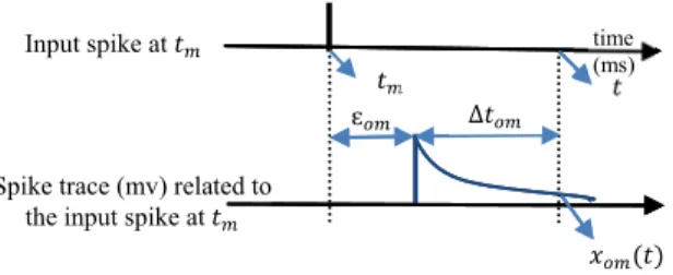
Fig. 1. Trace xomrelated to input spike at tm jumps to a maximum value
after the delayεom. Then it decays exponentially through time.
hidden neuron and the oth output neuron, and A is a constant value which are equal to their counterparts in (2). xoh(t) is
used to obtain appropriate value for delay adjustment. The adjustmentεoh is calculated by (4) similar to EDL [43]
εoh(t)= ⎧ ⎪ ⎨ ⎪ ⎩ +tom(t)(xoh(t)/xom(t))4, t = ˆtof −tom(t)(xoh(t)/xom(t))4, t =tof 0, Otherwise (4)
where tˆof is the time of the f th desired spike, tof is the
time of the f th actual output spike of the oth output neuron, and xom(t) is the maximum trace between the traces of the
excitatory hidden neurons connected to the oth output neuron at the current time t. xom(t) is corresponding to the connection
between the mth excitatory hidden neuron (that has the closest spike before the current time t) and the oth output neuron.
tom is a delay shift which is necessary to be added to the
delay between the mth excitatory hidden neuron and the oth output neuron to bring the effect of the closest spike fired by mth excitatory hidden neuron to the current time t. It is derived from (3) and calculated by
tom=t−tm−εom= −τxln(xom(t)/A) (5)
where tm is the firing time of the mth excitatory hidden neuron
before current time t. The mth excitatory hidden neuron has the closest spike before the current time t. It has the maximum trace at time t xom(t)out of all excitatory input synapses of the
oth output neuron. xom(t)should be less than A, because the
spike should occur before the current time. εom is the delay
between the mth excitatory hidden neuron and the oth output neuron. Fig. 1 illustrates the relationship between the different parameters used in (5).
The delay adjustment in (4) tries to increase the total PSP of the oth output neuron at t = ˆtof and to reduce the total PSP
at t =tof. The delay increment in (4) shifts the positive PSPs
generated by excitatory inputs to the desired times to generate an output spike. The delay reduction shifts the positive PSPs away from the actual output spikes times to remove undesired spikes. When an actual output spike is generated at the time of a desired spike, the positive delay adjustment cancels out the negative delay adjustment and the delays are stabilized. In (4), we have [xoh(t)/xom(t)] ≤1. The use of the fourth
power in (4) reduces the amount of delay adjustment related to a far input spike. A far input spike corresponds to a low value of [xoh(t)/xom(t)] and consequently a lower value of
the fourth power of [xoh(t)/xom(t)] ≤1, and only the delays
related to the close input spikes which have a high effect on the PSP is adjusted by a high value to prevent unnecessary change of the delays in the network.
The adjustment of delay between the hth inhibitory hidden neuron and the oth output neuronμoh is governed by
μoh(t)= ⎧ ⎪ ⎨ ⎪ ⎩ −t¯om(t)(x¯oh(t)/(x¯om(t))4, t = ˆt f o +t¯om(t)(x¯oh(t)/x¯om(t))4, t =tof 0, Otherwise (6)
where x¯oh(t) is the spike trace related to the connection
between hth inhibitory hidden neuron and the oth output neuron.x¯om(t)is the maximum trace between the inhibitory
hidden neurons that are connected to the oth output neuron. It should be less than A. t¯om(t) is calculated by putting
¯
xom(t)in (5). The decrement of delays in the first expression
of (6) at the desired times shifts away the negative PSPs generated by inhibitory inputs (from the desired times) and increases the total PSP of the output neuron accordingly. This might increase the total PSP to hit the threshold level and generate an actual output at the desired times. The delay increment in the second expression relates to the inhibitory input spikes before the actual outputs shifts the negative PSP of the inhibitory inputs toward the actual output spikes to remove undesired output spikes. When an actual output spike is generated at the time of a desired spike, the delay decrement and increment in (6) are equal and the net adjustment becomes zero.
C. Training the Hidden Neurons
This section introduces the learning algorithms for both excitatory and inhibitory hidden neurons.
1) Weight Learning of Excitatory Hidden Neurons: The synaptic weight between the i th input neuron and the hth excitatory hidden neuron is denoted bywhi and all the delays
in the network are neglected in this stage. The synaptic weight adjustment is governed by whi(t) = ⎧ ⎪ ⎨ ⎪ ⎩ +o[(t−ti)(1−(t−th)/A)](woh/A), t= ˆtof −o[(t−ti)((t−th)/A)](woh/A), t=tof 0, Otherwise (7) where ti is the last firing time of the i th input spike at or before
the current time t. Equation (7) shows that the algorithm adjusts the weight at the time of the f th desired spike of the oth output neuron, t = ˆtof, and at the time of the f th actual
output spike of the oth output neuron, t=tof. The sigma (
)
collects the weight adjustment on all the output neurons. At the time of the desired spike, the weight is potentiated in proportion to the STDP time window ((t−ti)) to generate
hidden neuron spike at the desired time or shortly before it to increase the total PSP of the oth output neuron and help the output neuron to generate an actual output spike at the desired time (Fig. 2). Different hidden neurons correspond to different desired spikes, and they cooperatively force the output neuron to fire at all desired times.
Fig. 2. Synaptic weight between ith input neuron and the hth excitatory hidden neuron whi is potentiated in proportion to the value of STDP time window [(t−ti)] at t = ˆtof to generate hidden spike at the desired time t= ˆtof. The generated excitatory input will be fed to the oth output neuron,
and it increases the total PSP of the neuron at the desired time.
Fig. 3. whi, the synaptic weight between ith input neuron and the hth excitatory hidden neuron, is reduced in proportion to(t−ti), at t=tof (the
time of the f th actual output spike of the oth output neuron). The reduction might lead to the cancelation of the hidden spike at th and consequently the
reduction of the total PSP of the oth output neuron generated at t =tofand
remove the actual output at t=tof.
At the time of an actual output, t=tof,whi(t)is reduced
in proportion to the STDP time window(t−ti). It depends
on the time difference of its input spike ti, and the current time
t =tof, (tof−ti). The reduction might lead to the cancellation
of the hidden spike at th shortly before t =tof or at t f o, and
consequently reduces the total PSP of the oth output neuron generated at t = tof and remove the actual output at t =tof
(Fig. 3). When the actual output spikes at t =tof, it becomes
close to the desired spike at t = ˆtof, the positive weight
adjustment related to the desired spike cancels out the negative
weight adjustment at the actual output. Consequently, the net weight adjustment becomes small.
The excitatory hidden neuron weight is adjusted based on the three spikes shown in Fig. 3 by (7). In a triplet-STDP, which is a more accurate model of synaptic plasticity in a biological neuron than a standard pair-based STDP [1], three spikes also affect a weight adjustment. A triplet-STDP described in [1] uses a single presynaptic and two postsynaptic spikes. There are different models for triplet-STDP [1].
The term [(1−(t −th)/A)] in (7) prevents the weight change of an excitatory hidden neuron that already has an actual output at the desired time, t = ˆtof as in this situation (tˆof −th) = A, consequently, [(1−(tˆof −th)/A) = 0].
Therefore, the weight increment related to the hidden whi
is 0, because the hidden neuron already has a spike at this desired time and it does not need more weight adjustment. Different hidden neurons contribute to firing of the output neuron at different desired times and cooperatively help the output neuron to fire at all the desired spikes in a multispike coding scheme. The term also causes a smaller increment of the weightwhi that has output spike closely before the desired
spike [(tˆof−th)∼= A, consequently,(1−(tˆof−th)/A)∼=0].
An unnecessary high adjustment might shift the hidden spike close totˆof beyond the desired time and reduce the total PSP of
the oth output neuron at the desired time. In addition, the term
(1−(t−th)/A)causes a comparatively high increment of
whi when a hidden neuron does not have spike before t = ˆtof
[because (1−(tˆof −th)/A) = 1], or the actual output of
the hth hidden neuron is far from the desired time at t = ˆtof
[(1−(tˆof −th)/A)∼= 1]. The high increment might force
the hth hidden neuron to fire at the desired time t = ˆtof, and
consequently increase the total PSP of the oth output neuron at the desired times t= ˆtof.
The term [(t −th)/A] in (7) when t = tof prevents the
reduction ofwhi if the hth excitatory hidden neuron does not
have any actual output spikes before the actual output of the oth output neuron at t =tof [((tof −th)/A)=0]. Because, whi does not have any roles in the generation of the output
spike at t = tof. If an excitatory hidden neuron has output
spike before and close to an actual output spike at t = tof,
the term has comparatively a high value [((tof−th)/A)∼=1],
and consequently,whiis adjusted with a higher value, because
the excitatory hidden neuron has a strong contribution in the generation of the actual output spike at t =tof and the weight
reduction might lead to the removal of the output from the excitatory hidden neuron and consequently reduce the total PSP of the output neuron.
In a network with nonzero delays, the proposed method trains the excitatory hidden neuron to fire at a time interval (equal to the corresponding delay connecting the hidden neuron to the output neuron) before a desired time. The early firing of the excitatory hidden neuron increases the total PSP of its successor output neuron at the desired time by the delayed effect of the excitatory hidden spike. However, in the previous situation, where the connections do not have any delays, an excitatory hidden neuron is trained to fire at the same time as the desired time. Correspondingly, (8) is used to
adjustwhi, the synaptic weights between the i th input neuron
and the hth excitatory hidden neuron, at time t
whi(t) = ⎧ ⎪ ⎨ ⎪ ⎩ +o[xhi(t−εoh)(1−xoh(t)/A)](woh/A), t = ˆtof −o[xhi(t−εoh)(xoh(t)/A)](woh/A), t =tof 0, Otherwise (8) where xhi(t) is the spike trace corresponding to the connection
between the i th input neuron and the hth excitatory hidden neuron. Each spike in the i th input spike train causes a delayed (εhi) jump in the trace then it decays exponentially
by a time constant similar to (3). xoh(t) is the trace
corre-sponding to the connection between the hth excitatory hidden neuron and the oth output neuron. Each output spike of the hth excitatory hidden neuron results in a delayed (εoh)jump
in the trace which decays exponentially by a time constant τ similar to (3). εhi is the delay between the i th input neuron
and the hth excitatory hidden neuron, and εoh is the delay
between the hth excitatory hidden neuron and the oth output neuron. The traces have same amplitude A and time constantτ as the STDP time window in (2).
The update of whi at t = ˆtof in (8) based on the delayed
xhi(t) increases whi by a high value if it has spike shortly
before (tˆof −εoh), because in this case xhi(tˆof −εoh) has a
high value. The high increase can lead to the generation of an output spike of the hth excitatory hidden neuron at(tˆof−εoh).
The effect of the generated hidden spike is shifted to the time of the desired spike in the oth output neuron after the delay of the connection between the hth excitatory hidden neuron and the oth output neuron εoh. This helps the output neuron
to generate output spike at the desired time.
The decrement in the second expression of (8) is high if the i th input neuron has spike shortly before (tof −εoh).
Consequently, this decrement tries to remove the actual output of the hth excitatory hidden neuron at (tof −εoh) and helps
the oth output neuron to reduce its PSP at the time tof (by
considering the delay εoh).
2) Weight Learning of the Inhibitory Hidden Neurons: The connection weight between the hth inhibitory hidden neuron and the i th input neuron w¯hi is updated similar to (8) by
multiplying it with a negative sign as shown in
w¯hi(t) = ⎧ ⎪ ⎨ ⎪ ⎩ −o[ ¯xhi(t−μoh)(x¯oh(t)/A)]|woh/A|, t = ˆtof +o[ ¯xhi(t−μoh)(1− ¯xoh(t)/A)]|woh/A|, t =tof 0, Otherwise (9) where μoh is the delay between the hth inhibitory hidden
neuron and the oth output neuron, and x¯hi(t) is the spike
trace corresponding to the connection between the i th input neuron and the hth inhibitory hidden neuron. x¯oh(t) is the
spike trace related to the connection between the hth inhibitory hidden neuron and the oth output neuron. The delay related the connection between the i th input neuron and the hth inhibitory hidden neuron isμhi. According to (9), the weight is reduced
if the i th input neuron has a delayed (μhi)spike shortly before
(tˆof −μoh)to increase the total PSP of the oth output neuron
at the desired time tˆof by removing hidden inhibitory spike
at or before (tˆof −μoh). In addition, (9) increases the weight
¯
whito generate hidden inhibitory spike at (tof−μoh)to reduce
the total PSP of the oth output neuron at t=tof. The reduction
of the total PSP removes the actual output spike of the oth output neuron at tof.
It is proposed that hidden neurons receive biofeedback from the readout neurons. Through this biofeedback, the times of desired spikes and actual outputs related to the neurons in the next layer are made available at the hidden layer neurons which use them to adjust their weights appropriately. In this paper, we did not describe the basis of the biofeed-back or model it in detail. The training of the network is stopped when it reaches its goal, i.e., the readout neuron generates actual output spikes at the desired times and all the undesired output spikes of the readout are removed.
D. Classification Ability of the Proposed Method
The weight and delay learning characteristics of the pro-posed method enable it to train a neuron to fire at desired spike times related to an applied input pattern. In a classification task, an input pattern is assigned to the class whose desired spike train is most similar to the actual output of the network. Therefore, the classification ability of the proposed method can be improved if an output neuron is also trained not to fire close to the desired spikes of other classes in addition to firing at the desired times representing to the current class of the input pat-tern. As a result, the proposed method introduces an additional learning mechanism when a misclassification occurs.
The learning algorithm considers two desired spike trains after a misclassification. The first one is related to the class of the applied input spatiotemporal pattern, i.e., the desired spikes of the correct class, and the second one is related to the class that causes the misclassification (incorrect class). Thus, the learning adjusts the readout neurons and hidden neurons learning parameters at the time of each desired spike related to the class that causes the misclassification. It reduces the weights of the readout neuron that have a spike before the desired time. To force the oth output neuron to not fire at the f th desired spike of class j (t = ˆtof(j))the weights of
the othoutput neuron are adjusted by the following equation at t = ˆtof(j):
woh(t)= −(t−th−doh). (10)
The proposed classification learning method adjusts an excitatory hidden neuron weight at the desired spike times (t = ˆtof(j))related to the class that causes the misclassification
by the following equation similar to (8):
whi(t)= −
o
[xhi(t−εoh)(xoh(t)/A)](woh/A). (11)
An inhibitory hidden neuron weight at t = ˆtof(j)is adjusted
similar to (9) by the following equation:
w¯hi(t)= +
o
The delay related to an excitatory input of a readout neuron is adjusted by (13) at t = ˆtof(j). The following equation is
similar to (4):
εoh(t)= −tom(t)(xoh(t)/xom(t))4 (13)
The delay related to an inhibitory input of the readout at t = ˆtof(j) is adjusted through the following equation which is
similar to (6):
μoh(t)= +t¯om(t)(x¯oh(t)/x¯om(t))4. (14)
The proposed method uses a criterion to control the learning level of every pattern and manage the misclassifications during training and adjust the network learning parameters to increase the inter class separability of the network.
Consider a pattern from class i is applied to the network and an actual output of the network is generated. The correlation between the actual output and the corresponding desired spike train of the class i is called ci which is calculated by the
method used in [41] as in
ci = vd·vo
|vd||vo| (15)
where “vd·vo” denotes the inner product of the two vectorsvd andvo.vd andvo are two vectors with real value components which are generated from spike trains. A desired spike train is convolved with a symmetric Gaussian function to generatevd. Similarly,vois generated by convolving an actual output spike train with the symmetric Gaussian function. |v| is the length of a vectorv.
A maximum value p and a threshold level c for ci are
considered to control the learning. If the correlation metric ci
is less than c, the network learning parameters are updated based on the applied training pattern and their desired spike train without considering any extra criteria. In this situation, the network adjusts its learning parameters to increase its knowledge about the applied training pattern inside the class i . The low value of the correlation related to the applied training pattern ci < c means that the similarity of the training
pattern with the previous trained patterns from the same class i is low and the learning parameters of the network should be adjusted to increase the ability of the network to recognize the patterns inside the class i .
If ci reaches the value of p, the learning related to the
pattern is not applied to the network in the current learning epoch, because the high value of the correlation shows that the knowledge of the presented training pattern is already in the network and it is not necessary to adjust the learning parameters for the current value of ci. It means that the
network has learned the overall distribution of the data from the class i and it is not necessary to memorize all the details of the presented training pattern. It also prevents over training of the network.
If ci has a value betweenc and p, i.e., (c<ci < p),
and ci is appropriately higher than the correlation metric
related to the other classes to prevent misclassification, then the learning related to the applied pattern is stopped in the current epoch. Therefore, if c<ci < p and ci >cj +c
(where j = argmax{k∈{1,2,...,N}&k=i}ck, ck is the correlation
TABLE I
PROPOSEDCLASSIFICATIONLEARNINGMETHOD
metric of the actual output with the kth desired spike train, and N is the number of all the classes), the learning adjustment related to the applied pattern from class i is not applied to the network in the current epoch. The ci >cj+c
denotes that the network can distinguish the class of the applied pattern correctly with an appropriate margin (c), therefore it is not necessary to have more training for the current value of ci in the learning epoch.
If ci has a value between c and p, and ci < cj +c,
it suggests that a misclassification has occurred. In this situa-tion, the network learning parameters are updated to enhance the interclass separability of the network by training it to not fire close to the desired spike train of the class that causes this misclassification and to reduce cj. The learning parameters are
also updated to increase the ability of the network to generate the desired spike related to the applied pattern from the class i to increase ci. The reduction of cj and the increment of ci
may change the situation ci <cj+c to ci >cj+c and
prevent the misclassification. The training is continued until the maximum number of learning epochs is reached or if the stopping criteria noted in Table I apply.
A ci greater than p shows that the network is trained to fire
appropriately close to the corresponding desired spike train. Therefore, similar to the situation where (c <ci ≤ p and
ci >cj+c)the related learning adjustment is not applied
to the network. The p value is chosen high enough depending on the desired spike trains related to the different classes to guarantee that when ci >p, ci is appropriately higher than cj
(ci >cj+c). Desired spike trains related to different classes
(related to ciand cj)should be chosen in a such a way that the
correlation between the desired spike trains are low enough to support the point that if an actual spike train is very similar to the desired spike related to ci, (ci >p)then it is appropriately
dissimilar to the other classes (cj <ci−c). The values of
p and c are determined by trial and error. In this paper, the method used in [44] is employed to choose the desired spikes. A sequence of numbers starting from 10 to 100 ms
with 10-ms time interval is generated. Then a number of firing times are extracted randomly from the sequence to assign each desired spike train corresponding to a class. In this situation, every two spikes have at least 10-ms interval. The parameter p is set based on the level of precision that the desired spikes should be learned. In this paper, when an actual output spike train reaches 90% of accuracy compared to its corresponding desired spike train the learning is stopped, so the learning parameter p is set 0.9. The parameter c should be higher than the maximum correlation between the desired spike trains related to different classes. c is set 0.45 to implement the proposed method.
After training, each testing pattern is applied to the network and the readout actual output spike train is calculated. The correlations between the actual output spike train and the desired spike trains corresponding to all classes are obtained. The input pattern is assigned to the class whose corresponding desired spike train has the maximum correlation value with the actual output spike train.
IV. RESULTS
A. Effect of Network Setups on the Learning Performance First, the effects of the different maximum allowable delays and the number of desired output spikes in each class on the performance of the learning method are explored. Then, the running time for the proposed method is reported. In the following simulation, the performance of the network is first evaluated on the Fisher IRIS data set. The IRIS data fea-tures are converted to spike times using population coding, as described in [23], where each feature value is encoded by M identically shaped overlapping Gaussian functions where M is set to 40. The IRIS data have four features for each pattern so there are 4×M =160 input spikes obtained which are then applied to 160 input synapses. The high number of input synapses increases the number of input spikes, and consequently reduces the length of silent windows inside a spatiotemporal input pattern and helps the neuron to fire at multiple desired times. In addition, there are nine extra input synapses with input spikes at fixed times for all patterns. The fixed times are the same as the times of desired spikes cor-responding to all classes. These inputs act as bias inputs [21] and act as the reference start times in a multispike coding scheme. There are 360 hidden neurons in the hidden layer. The total time duration of the input spatiotemporal pattern is set to 100 ms, T =100 ms.
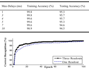
1) Effect of Maximum Allowable Delays: Similar to [24], 50% of the IRIS data were selected randomly and used as training data and the remaining used for testing. The accuracy of the proposed method on the testing data reaches its highest value, 95.1%, when the maximum allowable delay D is 3 ms and there is a single readout neuron.
In Table II, the accuracies of the proposed method for different delays when there are three readout neurons (each corresponding to a class) in the network are shown. The accu-racy of the method on the testing data reaches its maximum value when D=3 ms (Table II). The accuracy of the proposed method on the testing data is increased from 95.1% to 95.7%
TABLE II
EFFECT OF THEDIFFERENTMAXIMUMALLOWABLEDELAYS ON
IRIS DATARECOGNITION. 50%OF THEDATAARE
USED ASTRAININGDATA
Fig. 4. Comparison of the learning method accuracy on the IRIS data training set when one and three readout neurons are used.
when the number of readout neurons is increased from one to three when D = 3 ms. In Fig. 4, the accuracy of the learning algorithm on the training data is shown when a single readout neuron and three readout neurons are used. All these procedures are repeated independently for 40 different runs, and the mean value of the 40 results are reported. Different random initial weights and different random selections of the training and testing data are used for the different runs. When the number of readout neurons is increased, the number of learning parameters is also increased. Therefore, the readout neurons learn a lower number of training patterns compared to the situation where a single readout neuron is used, where the readout neuron should learn patterns related to all classes. Subsequently, they can learn the input patterns better compared to the situation that a single readout neuron is used. For higher values of maximum allowable delays, the cooperation between weight adjustment and delay adjustment is reduced and it leads to a lower accuracy. A higher delay adjustment causes a higher shift in the delayed effect of input spikes, and this higher shift might destroy previous weight training that was based on the previous value of the delay.
Synaptic delays at chemical synapses usually take values from 1 to 5 ms. The minimum value of a synaptic delay is 0.3 ms. Synaptic delay also can take a value higher than 5 ms [45]. Different researchers use different maximum values for range [1, 16] ms. The results in this section show that for this configuration, 3 ms is an optimal value for the maximum synaptic delay. In the following simulations, Max Delays are set to 3 ms.
2) Effect of the Number of Desired Spikes: In the following experiment, the accuracy of the proposed method is obtained for different numbers of desired spikes corresponding to each class (Table III).
The network reaches its maximum testing accuracy, 95.7%, when three desired spikes are used in each desired spike train.
TABLE III
EFFECT OF THENUMBER OFDESIREDSPIKES ONLEARNINGACCURACY
USING THEIRIS DATASETWITHTHREEREADOUTNEURONS
Fig. 5. Recognition accuracy for different numbers of desired spikes.
A very high number of desired spikes in each desired spike train (i.e., for a desired spike train with 100-ms duration and 10-ms minimum interspike interval, the highest number of desired spikes is 10) reduce the performance of the learning method as this increases the complexity of the learning task and the network should be trained to fire at a higher number of desired instances with a limited number of learning parame-ters. For instance, the testing accuracy of the proposed method is reduced from 95.7% to 81% when the number of desired spikes is increased from 3 to 7 (Fig. 5).
The time distances between desired spikes of different classes are reduced when there is a high increase in the numbers of desired spikes. Therefore, a small deviation in the times of output spikes can cause a switching from one class to the other one and reduces the accuracy. On the other hand, a lower number of desired spikes reduce the complexity of the learning task, therefore the training accuracy will be increased. However, a very low number of desired spikes lead to a low testing accuracy. For example, when the number of desired spikes is reduced from three to one, the testing accuracy is reduced from 95.7% to 95.1%. It shows that a single spike cannot capture enough information from training data, and consequently, it reduces the testing accuracy despite of a comparably high training accuracy of 99.9%. Moreover, the distributions of spikes in the spatiotemporal input patterns compared to desired spikes also affect the accuracy and the relation between the number of desired spikes, and the accuracy is not a simple linear function (Fig. 5).
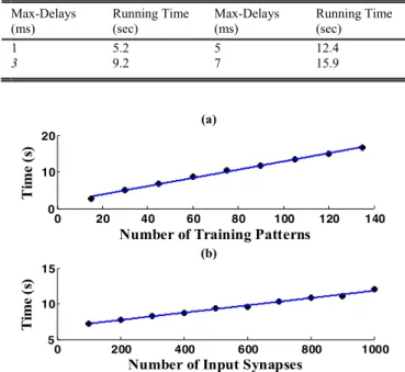
3) Evaluation of the Running Time: MATLAB simulations were carried out on a quad core PC with 3 GHz and 16 GB of RAM. The running times required for each learning epoch of the proposed method are reported in Table IV. The running time related to a learning epoch is measured 10 times, and the mean value is reported for each number of input synapses. The running time is increased by increasing the maximum allowable delays D. For instance, the method needs 5.2 s to execute a learning epoch when D = 1 ms. However,
TABLE IV
EFFECT OF THEMAXIMUMALLOWABLEDELAY(d)ON THERUNNING
TIME OF THEPROPOSEDMETHODUSING THEIRIS DATASET
Fig. 6. Runing time of a learning epoch is increased linearly as a function of (a) number of training patterns and (b) number of input synapses.
the running time is increased to 15.9 s when D is increased to 7 ms. Because, at each time step, the learning algorithm should check the events at the previous time steps depending on the delays. A higher number of previous time steps should be considered for a higher value of delays. Therefore, the computational complexity of the method and consequently the running time is increased when the delay is increased.
The running times of a learning epoch of the proposed method are measured for different numbers of training pat-terns. The number of training patterns is increased from 15 to 135. IRIS data set is used to train the algorithm. Fig. 6(a) shows the relationship between the running times and the number of training patterns. The fit line shown in Fig. 6(a) is obtained by fitting the data points to a 1-D polynomial. The line is described by the equation T(n) = 0.1128n+1.593. The time complexity of the process related to the equation is linear, i.e., it is O(n)using the big O notation. It shows that the running time increases linearly with the number of training samples.
Random spatiotemporal input patterns with different numbers of inputs are used to analyze the complexity of the learning algorithm as a function of the number of input synapses. There are three classes similar to IRIS data in the randomly generated data. A spike train composed of three spikes is considered as desired spike train for each class like the desired spike used for IRIS data. The spike times in each input spatiotemporal pattern are generated by a uniform distribution. The values of spike times are extracted randomly from (0, 100) interval. The number of input synapses is changed from 100 to 1000, and an input spike is considered for each input synapse. Then, the running time for each
TABLE V
COMPARISONWITH THEMULTILAYERSNN PROPOSED IN[28]ON THEIRIS DATASET
learning epoch is calculated to analyze the complexity of the learning method. In this experiment, there are a fixed number of 75 training patterns. Fig. 6(b) shows the evolution of the running time in terms of the number of input synapses. In addition, a line fit with the obtained data points is plotted. The dependence between running time and the number of inputs indicates a linear time complexity, i.e., O(n).
B. Comparison With State-of-the-Art Methods
In the following simulation, first the proposed method is compared with the method proposed by Sporea and Grüning [28]. In this case, 75% of the total IRIS data for each class are considered as a training set and the remaining 25% are used for testing, as in [28]. The results are shown in Table V. The accuracy of the proposed method on the training is 99% which is higher than the method proposed in [28], 96%. The proposed method also achieved a higher testing accuracy of 96% (compared to 94% achieved by [28]).
Similar to the biologically plausible structure used in [18], each of the 169 input neurons is connected randomly to a limited number of neurons (40 neurons) in the hidden layer which consists of a population of 360 neurons. There are no subconnections, and every two neurons in two subsequent layers are connected by a single connection similar to the bio-logically plausible neural network in Izhikevich’s work [18]. The proposed learning algorithm is designed to manage the training of a large number of SNs by local events such as spike trace which takes place at the location of each synapsis. There are three output neurons in the output layer and all the hidden neurons are connected to the three output neurons. The network proposed in [28] uses the timing of a single spike of an input neuron for each feature. The four input neurons are fully connected to ten neurons in the hidden layer. Every two neurons in two subsequent layers are connected by 12 subconnections with different delays from 1 to 12 ms. All the neurons in the hidden layer are fully connected to an output neuron. The performance of the method in [28] on the IRIS data is shown in Table V.
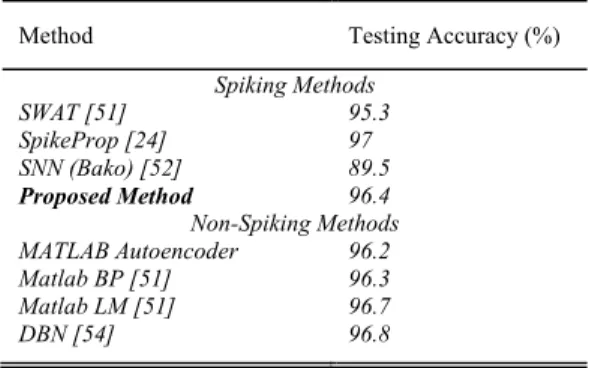
In order to compare the accuracy of the proposed method with that achieved by other existing methods, 50% of the data samples from the IRIS data set are selected randomly to construct training data and the remaining 50% are used for testing. The testing results are summarized in Table VI. The accuracies of the proposed method on the training and testing data are 99.7% and 95.7%, respectively. The testing accuracy of the proposed method, 95.7%, is comparable with the best
TABLE VI
COMPARISONWITHOTHERMETHODS ON THEIRIS DATASET
TABLE VII
COMPARISONWITHOTHERMETHODS ON THEWBCD DATASET
result achieved for the state-of-the-art methods on IRIS data set. The proposed method has a high training accuracy, 99.7%. The proposed method converges for all trials because it does not have the silent neuron problem. It has remote supervised spikes. In addition, it solves the problem of silent windows in a spatiotemporal input pattern by delay learning. A silent window can prevent generation of desired spikes and con-sequently it can cause learning convergence problem. These characteristics of the proposed method make it appropriate for learning multiple spikes. The accuracies of the proposed method are calculated for all trials, and there are not any rejected results. In contrast, the convergence rate of SpikeProp is investigated in [24] and as it has a problem with silent neurons it cannot converge for all trials, and as a result, those trials with low accuracies are removed from the reported results [24].
The Breast Cancer Wisconsin (Diagnostic) data set (WBCD) from the UCI machine learning repository is used as the sec-ond data set to evaluate the proposed method and to compare it with the other state-of-the-art methods, as shown in Table VII. WBCD contains 699 samples. The samples belong to two different classes (malignant and benign categories) where 458 samples are from the first category and 241 samples are from the second category. A total of 120 samples are selected
TABLE VIII
PERFORMANCECOMPARISONWITHSRESNANDGPSNN
ON THEBUPA LIVERDISORDERSDATASET
Fig. 7. Evolution of the accuracy of the proposed method over different learning epochs on BUPA liver disorders data. It needs 24 learning epochs to pass the accuracy level of 60%. SRESN [46] needs 715 epochs to reach about to the same level of accuracy.
randomly from each category to construct the training set, and the remaining data is used for testing. The proposed method has an accuracy comparable with the best accuracy achieved by the other state-of-the-art methods (Table VII).
One advantage of SNNs is that they use spikes to commu-nicate between neurons. However, in the classical neural net-works, real values are used to transfer data between neurons. Each spike can be encoded by a binary bit; however, a real value needs a high number of bits to be transferred between neurons depending on the precision that is required for the values. As shown in Tables VI and VII, the proposed method using spikes for communication between neurons and can achieve better or comparable accuracies with the state-of-the-art rate-based models including deep belief network (DBN) and autoencoders.
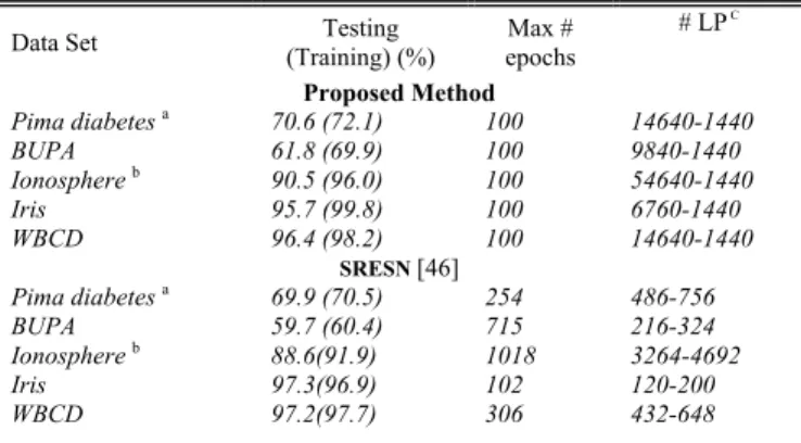
One more data set which is used to evaluate the proposed method is the BUPA liver disorders data from the UCI machine learning repository. There are 345 samples in this data set in which 145 samples are from the first class and 200 samples are from the second class. A total of 70 data samples are selected randomly from each class to construct the training set, and the remaining data is used for testing. Each sample has six attributes. The performance of the proposed method is shown in Table VIII. The testing accuracy of the proposed method is higher than self-regulating evolving spiking neural classifier (SRESN) [46] and growing-pruning spiking neural network (GPSNN) [47]. SRESN [46] uses a 30-2 architecture, and the proposed method uses a 246-360-2 architecture where there are 246 input neurons, 360 hidden neurons, and two output neurons. The evolution of the training accuracy of the proposed method over different learning epochs is shown in Fig. 7. The proposed method needs 24 learning epochs to pass the training accuracy of 60.4%; however, SRESN [46] needs 715 learning epochs to reach the same accuracy level. The proposed method can reach the accuracy level of 66.9% in less than 100 epochs. The performance of the proposed method on different data sets is compared with SRESN [46] in Table IX. The number
TABLE IX
COMPARISONWITHSRESNONDIFFERENTDATASETS
of learning parameters in SRESN [46] is lower than that of the parameters in the proposed method (see Table IX). A lower number of learning parameters can reduce the simulation time required for each learning epoch. However, the proposed method achieved high accuracies in a lower number of learn-ing epochs compared to the method with a slearn-ingle layer of learning neurons on Pima diabetes, BUPA liver disorder, and ionosphere data sets. The proposed learning method achieves this improvement through appropriate interaction between different layers of SNs in a multilayer structure.
V. CONCLUSION
This paper proposed a BPSL for multilayer SNNs. It uses the precise timing of multiple spikes, which is a biologically plausible information coding scheme. The learning parameters of neurons in the hidden layer and output layer are learned in parallel using STDP, anti-STDP, and delay learning.
The simulation results show that the proposed method has improved the performance of the first fully supervised algorithm that learns multiple spikes in all layers proposed in [28].The improvement of the proposed method can be attributed to a number of properties of the proposed method. First, it has used the firing times of spikes fired by the hidden neurons to train the weights of the hidden neurons unlike the method in [28] where the firing time of hidden neurons is not considered and the weights of a hidden neuron are adjusted by the same values irrespective of the neuron firing at the desired times or not firing at all. In the proposed method, weight learning, based on the firing times of the hidden neurons, helps adjust the weights appropriately and prevents unnecessary weight adjustments. Another property of the proposed method is the appropriate use of the EPSP and the IPSP produced by the hidden excitatory and inhibitory neurons to effectively adjust their weights, unlike the approach in [28] where equal weight updates are applied to both excitatory and inhibitory neurons, which can reduce the learning performance. Another property of the proposed method that improves its performance compared to the learning method in [28] is the appropriate