High Dimensional Regression Techniques for Complex Data

Clemson University

Clemson University

TigerPrints

TigerPrints

All Dissertations

Dissertations

December 2019

High Dimensional Regression Techniques for Complex Data

High Dimensional Regression Techniques for Complex Data

Chase Joyner

Clemson University, [email protected]

Follow this and additional works at: https://tigerprints.clemson.edu/all_dissertations

Recommended Citation

Recommended Citation

Joyner, Chase, "High Dimensional Regression Techniques for Complex Data" (2019). All Dissertations. 2503.

https://tigerprints.clemson.edu/all_dissertations/2503

This Dissertation is brought to you for free and open access by the Dissertations at TigerPrints. It has been accepted for inclusion in All Dissertations by an authorized administrator of TigerPrints. For more information, please contact [email protected].

H

IGH DIMENSIONAL REGRESSION TECHNIQUES FOR COMPLEX DATA

A Dissertation Presented to the Graduate School of

Clemson University

In Partial Fulfillment of the Requirements for the Degree

Doctor of Philosophy Statistics by Chase Joyner December 2019 Accepted by:

Dr. Christopher McMahan, Committee Chair Dr. Andrew Brown

Dr. Brook Russell Dr. Xiaoqian Sun

Abstract

This dissertation focuses on developing mixed effects models for large scale and complex data. Our motivating applications involve areas where this data is common, including epidemiological studies, environmental sciences, and genetics. Two key attributes for most of the modeling techniques discussed in this dissertation are that they scale easily to large data and that they achieve full variable selection, which is often a desirable trait in mixed effects models. These attributes are primarily handled in two ways. The first is with carefully constructed latent variables that we introduce to make the posterior distributions more tractable. This allows a Markov chain Monte Carlo (MCMC) sampler to be carried out with Gibbs steps, which results in efficient computation of posterior estimates, especially in large data scenarios. The second is through a decomposition of the covariance matrix associated with the random effects and with the use of spike and slab priors, we can achieve full variable selection in not only the fixed effects, but also the random effects. The finite sample performance of our techniques are assessed through extensive simulations and are used to analyze motivating data sets, which includes data from group testing procedures, human disease surveillance studies, and genetics.

Acknowledgments

Many thanks to my dissertation advisor, Dr. Christopher McMahan, without whom none of this work would have been possible. I would also like to thank the other members of my dissertation committee, Drs. Andrew Brown, Brook Russell, and Xiaoqian Sun for their feedback and advice throughout my dissertation. Much of this work was completed in collaboration with other co-authors. In addition to my committee members, I would like to thank the National Institute of Health, Biorealm Principal Investigator, and the National Science Foundation for funding individual pieces of this work.

Table of Contents

2 From mixed effects modeling to spike and slab variable selection: A Bayesian regression model for group testing data . . . 3

2.1 Introduction . . . 3

2.2 Notation and preliminaries . . . 5

2.3 Data augmentation and prior specification . . . 8

2.4 Posterior computation and inference . . . 11

2.5 Simulation . . . 14

2.6 Chlamydia testing application . . . 17

2.7 Discussion . . . 20

3 Mixed effects Bayesian regression for multivariate group testing data . . . 21

3.1 Introduction . . . 21

3.2 Methodology . . . 23

3.3 Simulations . . . 29

3.4 Data application . . . 32

3.5 Discussion . . . 33

4 A Bayesian Hierarchical Model for Identifying Significant Polygenic Effects while Controlling for Confounding and Repeated Measures . . . 35

4.1 Introduction . . . 35

4.2 Model . . . 37

4.3 Numerical Studies . . . 43

4.4 Application . . . 45

4.5 Discussion . . . 47

5 A two-phase Bayesian methodology for the analysis of binary phenotypes in genome-wide association studies . . . 49

5.1 Introduction . . . 49

5.2 Methodology . . . 51

5.4 Colorectal cancer data . . . 58

5.5 Discussion . . . 60

6 Discussion . . . 62

Appendices . . . 63

A Supplementary Material for Chapter 2 . . . 64

B Supplementary Material for Chapter 3 . . . 73

List of Tables

6.1 Simulation results with known assay accuracies (Sej= 0.95andSpj = 0.98) under the Dirac

spike. This summary includes the average bias of the posterior mean estimates (Bias), sample standard deviation of the posterior mean estimates (SSD), and the posterior probability of inclusion (PI). The total number of individuals isN = 5000with a common group size of4. The parameterdijdenotes theijth element ofD. . . 90

6.2 Simulation results with unknown assay accuracies under the Dirac spike. This summary includes the average bias of the posterior mean estimates (Bias), sample standard deviation of the posterior mean estimates (SSD), and the posterior probability of inclusion (PI). The total number of individuals isN = 5000with a common group size of4. The parameterdij

denotes theijth element ofD. . . 91 6.3 Analysis of the Iowa chlamydia data. This summary includes the posterior mean estimate

(Estimate), posterior standard deviation estimate (ESD), and the posterior probability of in-clusion (PI). The unstandardized effect estimate (β∗) is reported. . . 92 6.4 Simulation results with known assay accuracies (Sej:1 =Sej:2= 0.95andSpj:1=Spj:2=

0.98). This summary includes the average bias of the posterior mean estimates (Bias), sample standard deviation of the posterior mean estimates (SSD), and the posterior probability of inclusion (PI). The total number of individuals isN = 5000with a common group size of4. The average prevalence ratepfor each disease is reiterated. . . 93 6.5 Simulation results with unknown assay accuracies. This summary includes the average bias

of the posterior mean estimates (Bias), sample standard deviation of the posterior mean esti-mates (SSD), and the posterior probability of inclusion (PI). The total number of individuals isN= 5000with a common group size of4. The average prevalence ratepfor each disease is reiterated. . . 94 6.6 Analysis of the Iowa chlamydia data. This summary includes the posterior mean estimate

(Estimate), posterior standard deviation estimate (ESD), and the posterior probability of in-clusion (PI). . . 95 6.7 Simulation configuration 1: First set of randomly selected SNPs, for all considered values of

σ. Results were obtained through the GGDP and GDP models, as well as through applying the approach outlined in Armagan, Dunson, and Lee (2013). Presented results consist of the empirical bias (Bias), empirical mean-squared error (MSE), and sample standard deviation (SD) of the parameter estimates that were estimated as non-zero, as well as the percentage of the time that a coefficient was identified as being significant (Percent). Also included are the percentage of false discoveries (FDP) for each considered configuration and the average number of iterations the EM algorithm went through before convergence (Iter) with the aver-age time (measured in seconds) being provided in parenthesis. The minor allele frequency is also reported (MAF). . . 96 6.8 Data Application: Results include the estimated field and genetic effects on yield obtained

by the GGDP and GDP models. NS indicates that the SNP was not selected by a particular model and the minor allele frequency of the selected SNPs is reported (MAF). The prediction error (CVerror) is also provided, and was computed via 5-fold cross validation. . . 97

6.9 Simulation results whenn= 200andq2∈ {100,200,500}. The summary includes the

em-pirical bias (Bias) and standard deviation (SD) of the MAP estimates, as well as the percent of times the significant variable remained in the model (Perc). The SNP coefficients are cate-gorized according to their allelic frequencies (AF). The empirical false discovery proportion (FDP) for the truly unrelated variables is also included. The average times required to analyze each data set were 9.1, 12.6, and 46.9 seconds whenq2 = 100,200,500, respectively. This

time includes the grid search over the various(α, η)settings. . . 98 6.10 Simulation results whenn= 500andq2∈ {100,200,500}. The summary includes the

em-pirical bias (Bias) and standard deviation (SD) of the MAP estimates, as well as the percent of times the significant variable remained in the model (Perc). The SNP coefficients are cate-gorized according to their allelic frequencies (AF). The empirical false discovery proportion (FDP) for the truly unrelated variables is also included. The average times required to analyze each data set were 30.2, 36.1, and 85.8 seconds whenq2= 100,200,500, respectively. This

time includes the grid search over the various(α, η)settings. . . 99 6.11 Summary of the analysis of the Colorectal cancer data. Presented results include the

chromo-some number (Chr) and coordinate (Coordinate) of the identified SNPs, the gene they lie on (Gene), reference allele (Ref), minor allele frequency (MAF), and estimated effect (Estimate). 100 6.12 Simulation results with known assay accuracies (Sej = 0.95andSpj = 0.98) under SSVS.

This includes the average bias of the posterior mean estimates (Bias), sample standard devi-ation of the posterior mean estimates (SSD), and the posterior probability of inclusion (PI). The total number of individuals isN= 5000with a common group size of4. The parameter dijdenotes theijth element ofD. . . 101

6.13 Simulation results with known assay accuracies (Sej = 0.95andSpj = 0.98) under NMIG.

This includes the average bias of the posterior mean estimates (Bias), sample standard devi-ation of the posterior mean estimates (SSD), and the posterior probability of inclusion (PI). The total number of individuals isN= 5000with a common group size of4. The parameter dijdenotes theijth element ofD. . . 102

6.14 Average estimated area under the receiver operator characteristic curve for the proposed model and the competing model which ignores both variable selection and random effects. The known assay accuracies(Sej = 0.95andSpj = 0.98) setting (Known) is provided along

with unknown assay accuracies (Unk). . . 103 6.15 Simulation results with unknown assay accuracies under SSVS. This summary includes the

average bias of the posterior mean estimates (Bias), sample standard deviation of the posterior mean estimates (SSD), and the posterior probability of inclusion (PI). The total number of individuals isN = 5000with a common group size of4. The parameterdij denotes theijth

element ofD. . . 104 6.16 Simulation results with unknown assay accuracies under NMIG. This summary includes the

average bias of the posterior mean estimates (Bias), sample standard deviation of the posterior mean estimates (SSD), and the posterior probability of inclusion (PI). The total number of individuals isN = 5000with a common group size of4. The parameterdij denotes theijth

element ofD. . . 105 6.17 Analysis of the Iowa chlamydia data when using the Dirac spike and informative priors on

the testing accuracies. The summary includes the posterior mean estimate (Estimate), pos-terior standard deviation estimate (ESD), and pospos-terior probability of inclusion (PI). The informative priors were developed based on the product literature and validation trials avail-able on the Aptima Combo 2 assay and are given by:Se(1), Se(3) ∼Beta(196,13),Se(2) ∼

unstandard-6.18 The six models (M1-M6) with the highest posterior probabilities (see Kuo and Mallick; 1998) under both informative and uninformative prior specifications for the testing accuracies. Here x denotes that a variable is included in the model and Frequency denotes how often the model is visited. . . 107 6.19 Robustness study: Summary includes the average bias of the posterior mean estimates (Bias),

sample standard deviation of the posterior mean estimates (SSD), and the posterior probabil-ity of inclusion (PI). The total number of individuals isN = 5000with a common group size of4. The parameterdijdenotes theijth element ofD. . . 108

List of Figures

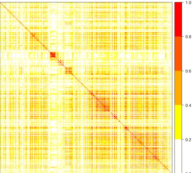
6.1 Graphical display of the correlation matrix between the 1232 SNPs in the data application. Darker shades indicate stronger correlation among genetic variants. . . 84 6.2 Graphical display of the genetic relatedness matrixCfor the 430 rice varieties. Darker shades

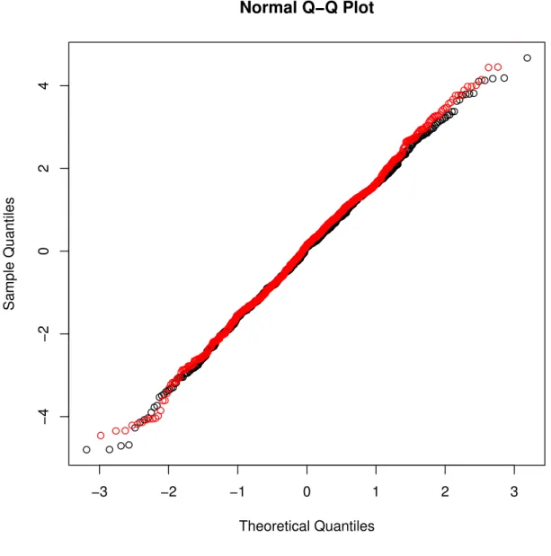
indicate varieties that are more genetically similar. . . 85 6.3 Normal QQ-plot of the residuals from the GGDP model (red line) and the GDP model (black

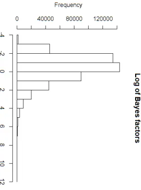
line) for the rice data. . . 86 6.4 Histogram depicting the natural logarithm of the Bayes factors which were computed for each

of 495,532 SNPs available in the CRC data. . . 87 6.5 Plot of the natural logarithm of the Bayes factors which were computed for each of 495,532

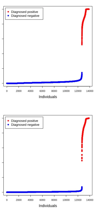
SNPs verses their position in the genome. Each shade change represents the transition to a new chromosome and the black triangles above the horizontal line depict the 200 SNPs with the largest Bayes factors. . . 88 6.6 The left (right) figure depicts the posterior infection probabilities for all individuals from

the Iowa chlamydia data corresponding to the analysis from Table 6.3 (Table 6.17) in the dissertation. The blue (red) points depict individuals who were diagnosed to be negative (positive). . . 89

Chapter 1

Introduction

Modern advancements in technology have allowed experimenters to gather and store larger amounts of data. While this advancement is favorable, it comes at the expense of more complicated modeling for statisticians. For example, special modeling techniques are required for the largepsmalln problems, or efficient modeling is necessary when eitherpor nare excessively large. These situations are practically ubiquitous in high dimensional analyses. High dimensional data is common in a variety of applications, including epidemiological studies, environmental sciences, and genetics. While more data can be a good thing, typical issues with high dimensional data arising from experimental designs in these areas are the number of predictors being considered (i.e., large p) or the complexity of the data. For example, group testing data arises in epidemiological studies, where the observed variables are often not on an individual level and also are error-contaminated observations due to imperfect testing. The latter issue is problematic as traditional binary data models are no longer valid, and the former issue further exacerbates the complexity of the required modeling framework. The Bayesian paradigm has proven most beneficial in these complicated models, and as such is used throughout this dissertation.

This dissertation primarily handles these complicated data structures in two ways. The first is that we utilize clever data augmentation strategies that make posterior distributions more tractable. For example, in binary regression, the addition of a carefully constructed latent variable allows the logistic or probit link function to be written into a normal distribution. The structure of these latent variables is inherently tied to the link function being used; e.g., follow Polson et al. [2013] and Albert and Chib [1993] for the logistic link and probit link, respectively. This allows model fitting to be carried out with primarily Gibbs steps, which provides for an efficient modeling framework that scales well to larger data. The second method used often in

this dissertation is variable selection. In complicated models, such as in mixed effects models, this becomes a major task as the dimensions of the parameter space grow quickly due to the inclusion of random effects. Chapter 2 develops a Bayesian mixed effects model that achieves full variable selection (i.e., in both fixed effects and random effects). Motivated by Chen and Dunson [2003], the variable selection within the random effects is achieved by placing spike and slabs priors on diagonal elements of a matrix that is the result of a Cholesky decomposition of the covariance matrix of the random effects.

In high dimensions, dimension reduction either before or during model fitting enables the analysis of large amounts of data. For example, Chapter 5 develops a two-phase methodology where the first phase prescreens the predictors to reduce it to a more promising set of candidates that are then jointly analyzed in the second phase. However, in some situations, it is more beneficial to jointly analyze all predictors simultaneously due to possible correlations and interactions. Chapter 4 develops a computationally efficient expectation-maximization that is motivated by Armagan et al. [2013a] and jointly analyzes large amounts of predictors by performing dimension reduction during the model fitting process. Due to the penalty structure of the prior used on the regression coefficients, once a regression coefficient is dropped from the model (i.e., is set to zero), it cannot return.

The remainder of this dissertation is organized as follows. Chapter 2 develops a Bayesian mixed effects logistic regression model for group testing data, where individuals of a population are screened for an infectious disease. Modern group testing procedures are moving towardsmultiplextesting assays, which have the ability to test for multiple diseases simultaneously. To account for this, Chapter 3 extends this model to a multivariate setting, which incorporates possible correlations between diseases. Chapter 4 develops a Bayesian linear mixed effects model that relates single-nucleotide polymorphisms (SNPs) of rice plants to the amount of yield produced. Chapter 5 involves developing a Bayesian logistic regression model to associate human SNPs and covariate information to colorectal cancer, where the number of predictors in the model is much larger than the sample size. We conclude with Chapter 6, a brief discussion of this dissertation.

Chapter 2

From mixed effects modeling to spike

and slab variable selection: A Bayesian

regression model for group testing data

2.1

Introduction

Group testing involves taking specimens (e.g., blood, urine, swabs, etc.) from different individuals and forming a pooled specimen that is then tested for disease. In most group testing protocols, if a pooled specimen tests negatively, then all individuals are declared to be disease free at the expense of a single diagnostic test. In contrast, if a pooled specimen tests positively, the pool is resolved algorithmically to determine which individuals are positive. Dorfman [1943] is credited with conceptualizing the group testing idea during World War II to screen military recruits for syphilis. Since then, group testing, or “pooling”, has become a mainstream approach to screen large populations for multiple diseases. The primary reason for pooling is to save money. For example, the State Hygienic Laboratory (SHL) at the University of Iowa has reported savings of approximately $3.1 million during a recent 5-year period after adopting a variant of Dorfman’s protocol to screen Iowa residents for chlamydia and gonorrhea; see Tebbs et al. [2013] and McMahan et al. [2017]. Pooling biospecimens through group testing arises in other applications, including testing for HIV and HCV [Sarov et al., 2007, Krajden et al., 2014], environmental testing [Heffernan et al., 2014], and drug discovery [Hughes-Oliver, 2006].

While testing pools can be far more cost effective than performing individual tests, it also leads to a more complicated data structure. This is true because specimens are pooled and hence individual-level re-sponses may never be observed. Recent statistical research has focused on developing regression methods to model the probability of disease for individuals based on pooled outcomes; e.g., see Vansteelandt et al. [2000], Bilder and Tebbs [2009], Huang [2009], Delaigle and Meister [2011], and Delaigle et al. [2014]. All of the aforementioned regression methods are designed to analyze test results arising from assaying the initially formed (master) pools; i.e., pools formed by assigning each individual to exactly one initial pool for test-ing. As a consequence, these methods cannot incorporate retesting information that becomes available when positive pools are resolved [Kim et al., 2007] or when quality control steps are implemented [Gastwirth and Johnson, 1994, Johnson and Gastwirth, 2000]. To incorporate retesting information, Xie [2001] developed an expectation-maximization algorithm to estimate the individual-level probability of disease for general re-gression models. Wang et al. [2014] developed a semiparametric framework to estimate single-index models. Most recently, McMahan et al. [2017] proposed a Bayesian approach to estimate generalized linear models while incorporating historical information on disease prevalence and uncertainty in assay performance.

At most public health laboratories like the SHL, individual specimens arrive at the lab from different locations throughout a particular geographic region. For example, in Iowa, specimens are collected at differ-ent types of clinics (e.g., family planning clinics, STD clinics, etc.) in multiple locations from all over the state and are then shipped to the SHL for testing. Given the vast differences among clinic types and the ad-ditional differences between rural and metropolitan areas, it is natural to suspect that heterogeneity may exist from location to location. However, when individual specimens are pooled together, it becomes a significant challenge to account for this source of variability while also estimating covariate effects like age, gender, race, and sexual history. In fact, most previous regression methods for group testing data, such as those outlined above, are not able to incorporate the effects due to observing data from different locations−especially when individual specimens from different locations are pooled together.

In this article, we develop a Bayesian generalized linear mixed model approach for group testing data which uses fixed effects to describe the population-level mean structure and random effects to account for differential variability among population subgroups. Our work generalizes the random effects model-ing techniques for group testmodel-ing data proposed by Chen et al. [2009] and simultaneously offers a far more

responses; i.e., it does not allow one to include additional retests that will be performed for disease classifi-cation purposes. On the other hand, our estimation framework is flexible and, as in McMahan et al. [2017], it can accommodate data from any group testing protocol as well as quality control screening procedures [Gastwirth and Johnson, 1994, Johnson and Gastwirth, 2000]. Third, and perhaps most limiting, the methods in Chen et al. [2009] allow only for pools to consist of individuals from within the same location. In prac-tice, this can be markedly prohibitive because individual specimens are often pooled sequentially based on their arrival date for testing. Furthermore, for those locations performing a small number of tests, it may be impractical to wait and to pool within location. Our approach removes this limitation and includes “pooling within location” as a special case. Finally, given the complexity of the considered mixed effects model, we use spike and slab priors to perform variable selection−both within the fixed and random effects components. In particular, three of the most common spike and slab priors are considered with details of implementation under each being provided. No existing group testing regression procedure has considered such an automated variable selection technique; i.e., for both fixed and random effects. For implementation purposes, a compu-tationally efficient Markov chain Monte Carlo (MCMC) sampling algorithm is developed which can estimate the proposed model.

Subsequent sections of this article are organized as follows. Section 2 provides preliminary infor-mation regarding the proposed mixed effects model, the modeling assumptions, and the derivation of the observed data likelihood. Section 3 presents the specifics of the approach, including prior model specifi-cations and data augmentation steps used to construct an efficient posterior sampling algorithm. Section 4 outlines the development of the full conditional distributions. Section 5 reports the results of an extensive numerical study conducted to assess the performance of the proposed approach. Section 6 presents an analy-sis of chlamydia testing data collected by the SHL in Iowa. Section 7 concludes with a summary discussion. Additional technical details and additional simulation results are provided in Appendix A.

2.2

Notation and preliminaries

Consider a setting in whichN individuals are screened for an infectious agent by a group testing protocol. As a part of this process, each of theNindividuals visit one ofKdistinct clinics, where a specimen (e.g., blood, urine, saliva, etc.) is collected. Testing is then performed either at the clinic site or at a regional laboratory; e.g., the SHL in Iowa. Note the former scenario would mandate pooling of individuals within clinic sites while the latter allows for pooling across sites, with our methodology being applicable in either

case. LetYei denote the true infection status of theith individual, fori = 1, ..., N, withYei = 1indicating

that the individual is truly positive andYei = 0otherwise. Furthermore, let xi = (1, xi1, ..., xi,q1−1)

0 _and

ti = (1, ti1, ..., ti,q2−1)

0 _{denote vectors of covariate values taken on theith individual which correspond to}

fixed and random effects, respectively, whereti is a subvectorxi. We assume throughout that individuals’

infection statuses are conditionally independent given the covariate information and the random effects. The individuals’ true infection statuses (i.e., theYei) are never observed due to the effect of imperfect testing,

while the covariate information for each individual is observed. For ease of exposition, we aggregate the individuals’ infection statuses asYe = (Ye1, ...,YeN)0 and denoteX= (x1, ...,xN)0andT= (t1, ...,tN)0 as

the design matrices.

The goal of this work is to relate the individuals’ latent infection statuses to their covariate values through the following generalized linear mixed model

g−1{P(Yei= 1|β,γk(i))}=x0iβ+t0iγk(i), (2.1)

whereg−1_{(·)is a known link function,βis aq}

1-dimensional vector of fixed effects,γk(i) :=γk if theith

individual presented at thekth clinic, andγk is aq2-dimensional vector of clinic-specific random effects,

fork = 1, ..., K. It is assumed that theγk are independent and identically distributed and follow a mean

zero multivariate Gaussian distribution with covariance matrixD; i.e.,γk iid

∼ N(0,D). Note, to track clinic membership, herein we adopt the functional notationk(·)and specify thatk(i) = k if theith individual presented at thekth clinic.

A typical challenge that arises in mixed modeling involves the selection of both the fixed and random effects components, which is tantamount to selecting the proper subsets of the available covariates to be retained in the final model. To accomplish this task, we adopt spike and slab priors [George and McCulloch, 1993, 1997, Kuo and Mallick, 1998]. These specifications proceed as usual for the fixed effects and follow the proposal of Chen and Dunson [2003] for the random effects, which requires a reparameterization of the proposed model. The reparameterized model is

g−1{P(Yei= 1|β,λ,a,bk(i))}=x0iβ+t 0

elements and free elements given byaml forl = 1, ..., q2−1;m = l+ 1, ..., q2. For ease of exposition,

we introduceλ = (λ1, ..., λq2)

0 _{such thatΛ=diag(λ)andawhich denotes the vector of free elements of}

the matrixA; i.e.,a = (aml:l = 1, ..., q2−1;m = l+ 1, ..., q2)0. Note that the matricesΛandAare

obtained via a modified Cholesky decomposition and satisfyD=ΛAA0Λ. Under this reparameterization, ifλl(thelth diagonal element ofΛ) is zero, then so is thelth diagonal element ofD. That is, ifλl= 0, then

the variance of thelth random effect is zero, which is equivalent to dropping thelth random effect from the model. Thus, to perform variable selection for the random effects, the proposed methodology places spike and slab priors on eachλl. Our approach also models theamlvalues, which allows for the estimation ofD

without imposing any prior form or structure.

The observed data that arises from implementing a group testing protocol can be quite complex. First of all, there are many protocols available for use [e.g., see Dorfman, 1943, Phatarfod and Sudbury, 1994, Kim et al., 2007, Kim and Hudgens, 2009]. Secondly, in an effort to reduce testing cost, a given protocol often requires that individuals be tested in multiple (possibly overlapping) pools and may even mandate confirmatory testing [Gastwirth and Johnson, 1994, Johnson and Gastwirth, 2000]. Thus, to provide a general framework which can incorporate and account for the complexity of data observed from implementing any group testing protocol, we define the index setPj⊂ {1, ..., N}which identifies the individuals contributing

to thejth pool, forj = 1, ..., J. LetZej denote the true status of thejth pool, under the convention that the

pool is positive (Zej = 1) if it contains at least one infected individual and negative otherwise (Zej = 0); i.e., e

Zj =I P_i∈PjYei >0

. Like the individuals’ true statuses, theZej’s are unobserved due to the effect of

imperfect testing. Instead, we observe the diagnosed statusZjwhich can be viewed as an error-contaminated

version ofZej, withZj = 1indicating that thejth pool tested positively andZj = 0otherwise. To quantify

the effect of imperfect testing, letSej = P Zj = 1 | Zej = 1

andSpj = P Zj = 0 | Zej = 0

denote the sensitivity and specificity, respectively, of the assay for thejth pool. We allowSej andSpj to be pool

specific, thus allowing for the potential use of different types of assays and/or the potential effect that pool size (i.e., the cardinality ofPj) may have on an assay’s performance.

To relate the individual-level model in (2.2) to the observed testing outcomesZ= (Z1, ..., ZJ)0, it

is assumed that the testing responses inZare conditionally independent givenZe= (Ze1, ...,ZeJ)0and that the

distribution ofZcan be written as π(Z|β,λ,a,b) = X e Y∈{0,1}N " J Y j=1 n SZj ej(1−Sej)1−Zj oZejn (1−Spj)ZjS 1−Zj pj o1−Zej × N Y i=1 g(ηi)Yie 1−g(ηi) 1−Yie # , (2.3)

whereηi=x0iβ+t0iΛAbk(i)andb= (b1, ...,bK)0. Note, on the right hand side of (2.3) we are

marginal-izing the joint conditional distribution of the observed testing responses and the latent statuses of the individ-uals, denoted byπ(Z,Ye | β,λ,a,b), overYe; i.e.,π(Z| β,λ,a,b) = P

e

Y∈{0,1}Nπ(Z,Ye | β,λ,a,b).

Unfortunately, (2.3) involves a very high dimensional sum effectively rendering direct numerical evaluation infeasible. To circumvent this issue, a two-stage data augmentation procedure in Section 3.2 is proposed which leads to an efficient posterior sampling algorithm.

2.3

Data augmentation and prior specification

The full hierarchy of the proposed model is

e Yi|ηi ∼ Bernoulli{g(ηi)}, ηi=x0iβ+t0iΛAbk(i) βq|vq ∼ (1−vq)πspike(βq) +vqπslab(βq), q= 1, ..., q1 λl|wl ∼ (1−wl)πspike(λl) +wlπslab(λl), l= 1, ..., q2 a ∼ N(m0,C0), bk ∼ N(0,I), k= 1, ..., K vq |τvq ∼ Bernoulli(τvq), q= 1, ..., q1 wl|τwl ∼ Bernoulli(τwl), l= 1, ..., q2 τvq ∼ Beta(av, bv), q= 1, ..., q1 τwl ∼ Beta(aw, bw), l= 1, ..., q2,

whereπspike(·)andπslab(·)denote the “spike” and “slab” components, respectively, of our spike and slab prior (for further details see Section 3.1) andm0,C0,av,aw,bv, andbware hyperparameters. In specifying

λl’s. Proceeding in this fashion greatly simplifies the calculations necessary for posterior sampling and is

common in the literature; e.g., see George and McCulloch [1993], George and McCulloch [1997], Kuo and Mallick [1998], and Chen and Dunson [2003].

2.3.1

Spike and slab prior

The model hierarchy presented thus far provides a general representation of the spike and slab prior. To ground the description of our approach and to illustrate our methodology, we discuss three commonly used spike and slab priors: the stochastic search variable selection (SSVS), the normal mixture inverse gamma (NMIG), and the Dirac spike, see George and McCulloch [1993], George and McCulloch [1997], and Kuo and Mallick [1998], respectively.

Following the work of George and McCulloch [1993], the SSVS approach used herein makes use of spike and slab priors of the following form:

βq |vq∼N(0, r(vq)φ2q) (2.4)

λl|wl∼T N 0, r(wl)ψl2,(0,∞)

, (2.5)

wherer(·)is a function serving as a binary switch (i.e.,r(0) = randr(1) = 1) that transitions the prior between the spike and the slab,φ2

qandψ2l are specified variance components, andT N(µ, ψ

2_{,(a, b))denotes}

the usual truncated normal distribution which arises from restricting the support of aN(µ, ψ2_{)distribution}

to the interval(a, b). In the specification of (2.4) and (2.5), one should provide large values ofφ2

q andψ2l

and a small value forr. In particular, these specifications should be made such thatr−1_{is sufficiently larger}

than the variance components; i.e., r−1 _{>> φ}2

q andr−1 >> ψ2l; for further discussion, see Wagner and

Duller [2012]. Proceeding in this fashion leads to a flat slab and a spike that is concentrated around zero. It is important to note that specifying appropriate values of the variance components can, in some instances, be challenging and moreover has the potential to greatly influence the analysis.

To avoid specifying the variance components, one could instead use the NMIG prior specification outlined in George and McCulloch [1997] and Ishwaran and Rao [2003]. This approach proceeds identically to that of SSVS with the exception that the variance components are viewed as unknown quantities and an inverse gamma prior is specified for them. That is,φ2

q ∼Inv-Gamma(aφ, bφ)andψ2l ∼Inv-Gamma(aψ, bψ).

This addition to the hierarchy removes the need to specify these nuisance parameters and allows one to esti-mate them through data driven means. One still must specify the value ofr; i.e., the proportional difference

between the variance components of the spike and slab densities. Experience suggests that the selection of rtends to impact the spike distribution far more than the slab, with the model selection process being too liberal whenris chosen too large and vice versa.

To avoid specifying r, a Dirac delta function could be used for the spike; see Kuo and Mallick [1998] and Wagner and Duller [2012]. This can be viewed as a limiting case of SSVS where the variance of the continuous spike distribution is driven to zero; i.e., r → 0. In this situation,vq = 0 if and only if

βq = 0and similarly forwlandλl. Although this seems favorable, it also introduces an absorbing state in

the Markov chain. To handle this issue, rather than sampling the binary variables from their full conditional distributions, βis integrated out when updatingv = (v1, ..., vq1)

0 _{andλis integrated out when updating} w = (w1, ..., wq2)

0_{. Thus, to develop a computationally efficient posterior sampling algorithm, one must}

be able to analytically marginalize the posterior distribution over bothβ andλ. The ability to do so is inherently tied to the link function being used. Fortunately, this can be accomplished under both the probit and logistic link functions after a series of data augmentation steps; this process is outlined in Section 3.2. The distribution for the slab can take on any diffuse continuous distribution. To closely mimic the slab priors in SSVS and NMIG, we takea prioritheβq’s to be independent with slab componentN(0, φ2q)and theλl’s

to be independent with slab componentT N 0, ψ2

l,(0,∞)

, whereφ2

qandψl2are again specified to be large.

2.3.2

Data augmentation

To facilitate the development of an efficient posterior sampling algorithm, a two-stage data aug-mentation procedure is proposed which focuses on impleaug-mentation under both the probit and logistic link functions. In the first stage, we introduce the individuals’ true statusesYe as latent random variables and

consider the joint conditional distribution of the observed testing responses and the latent statuses of the individuals, which is π(Z,Ye |β,λ,a,b) = J Y j=1 n SZj ej(1−Sej)1−Zj oZje n (1−Spj)ZjS 1−Zj pj o1−Zje × N Y i=1 g(ηi)Yei 1−g(ηi) 1−Yie .

individ-[2013]. In either case, this stage yields the following joint conditional distribution π(Z,Ye,ω|β,λ,a,b)∝ J Y j=1 n SZj_ej(1−Sej)1−Zj oZejn (1−Spj)ZjS 1−Zj pj o1−Zej ×exp −1 2(h−η) 0_Ω(h−η) N Y i=1 ξ(ωi), (2.6)

where ω = (ω1, ..., ωN)0 and η = (η1, ..., ηN)0. Under the probit link, h = (ω1, ..., ωN)0, Ω = I,

and ξ(ωi) = I(ωi ≥ 0,Yei = 1) + I(ωi < 0,Yei = 0). Under the probit link, ξ(ωi) acts to

con-trol the support ofωi such that givenYei = 0or 1 results in ωi being constrained to(−∞,0) or (0,∞),

respectively. Under the logistic link, h = (κ1/ω1, ..., κN/ωN)0, κi = Yei −1/2, Ω = diag(ω), and

ξ(ωi) = f(ωi | 1,0) exp{κi2/(2ωi)}, wheref(ωi | a, b)denotes the P´olya-Gamma density with

parame-ters(a, b); see Polson et al. [2013].

2.4

Posterior computation and inference

To facilitate estimation and inference, a posterior sampling algorithm consisting solely of Gibbs steps is constructed. In what follows, the necessary full conditional distributions used in this algorithm are provided. A symbolic representation of the entire posterior sampling algorithm is provided in Appendix A.1. Attention is first turned to the latent random variables introduced through the data augmentation pro-cedure. The full conditional distribution of the individuals’ latent statuses is given byYei |Ye−i,Z,β,λ,a,bk(i)∼

Bernoulli{p? i1/(p?i0+p?i1)}, where p?_i1=g(ηi) Y j∈Ii SZj ej(1−Sej)1−Zj p?_i0={1−g(ηi)} Y j∈Ii n SZj ej(1−Sej)1−Zj oI(sij>0)n (1−Spj)ZjS 1−Zj pj oI(sij=0) ,

sij =Pi0_∈Pj:i0_6=iYei0, and the index setI_i ={j:i∈ P_j}keeps track of the indices of the pools to which theith individual contributed. We also adopt the convention thatV−irepresents the vectorVafter removing

theith component. The full conditional distribution ofωiis link function dependent and is given by ωi|Yei,β,λ,a,bk(i)∼        T N{ηi,1,(0,∞)}, ifYei= 1, T N{ηi,1,(−∞,0)}, ifYei= 0, or ωi|β,λ,a,bk(i)∼PG(1, ηi),

under the probit and logistic link, respectively, where PG(a, b)denotes the P´olya-Gamma distribution with parameters(a, b); see Polson et al. [2013].

We now describe how to sample the fixed and random effects. Focusing on the quadratic form in the exponential in (2.6), we have that

(h−η)0Ω(h−η) = N X i=1 (hi−ηi)2Ωii = N X i=1 (hi−x0iβ−t 0 iΛAbk(i))2Ωii = N X i=1 (hβi−x0iβ) 2 Ωii= (hβ−Xβ)0Ω(hβ−Xβ),

whereΩii is theith diagonal element ofΩ,hβi = hi−t0iΛAbk(i), and hβ = (hβ1, ..., hβN)0. Thus, it

is easy to see that under the SSVS and NMIG spike and slab priors, the full conditional distribution ofβis given by β|Ye,ω,λ,a,b,v∼N n X0ΩX+Φ−1−1 X0Ωhβ, X0ΩX+Φ−1 −1o , whereΦ = diag r(v1)φ21, ..., r(vq1)φ 2 q1

. Under the Dirac spike, the full conditional distribution of βq

is degenerate at 0 if vq = 0, while the non-zero elements of β, sayβv, have the following normal full conditional βv|Ye,ω,λ,a,b,v∼N n X0_vΩX_v+Φ−_v1−1 X0_vΩh_β, X0_vΩX_v+Φ−_v1−1o ,

to the non-zero elements ofv. Due to the data augmentation steps described above, one can also obtain the following full conditionals

λl|Ye,ω,β,λ−l,a,b, wl∼T N{µλl(wl), σ2λl(wl),(0,∞)}

a|Ye,ω,β,λ,b∼N(µa,Σa)

bk|Ye,ω,β,λ,a∼N(µbk,Σbk),

where the specific forms of these distributions are provided in Appendix A.1. Sampling these parameters is equivalent to sampling the random effects as well as the covariance matrix of the distribution of the random effects.

For completion, the full conditional distributions ofvq andwlare Bernoulli, with the success

prob-ability depending on the specified spike and slab prior; see Appendix A.1. The full conditional distribu-tion for the mixing weights τvq and τwl are conveniently τvq | vq ∼ Beta(av +vq,1 −vq +bv)and

τwl | wl∼Beta(aw+wl,1−wl+bw), respectively. Finally, under the NMIG prior, the full conditionals

of the variance parameters areφ2

q |βq, vq ∼Inv-Gamma aφ+ 1/2, bφ+βq2/{2r(vq)}andψl2 |λl, wl∼

Inv-Gamma aψ+ 1/2, bψ+λl2/{2r(wl)}.

Up until this point, the assay accuracies (i.e.,SejandSpj) have been assumed to be known. When

these quantities are unknown, we may estimate them along with the rest of the model parameters following the approach outlined in McMahan et al. [2017]. Briefly, this approach allows for different assays to be used throughout the testing process (e.g., screening and confirmatory testing) and/or can account for the effect of pool size on the accuracy of the assay; i.e., sensitivity and specificity might change with the pool size. Define the index setMmwhich identifies the indices of the pools which were tested by themth assay, for

m= 1, ..., M. Further, letSe(m)andSp(m)denote the sensitivity and specificity of themth assay such that

Sej=Se(m)andSpj=Sp(m)for allj∈ Mm. Under these conventions, (2.6) can be written as

π(Z,Ye,ω|β,λ,a,b,Se,Sp)∝ M Y m=1 Y j∈Mm n SZj e(m)(1−Se(m))1−Zj oZjen (1−Sp(m))ZjS 1−Zj p(m) o1−Zje ×exp −1 2(h−η) 0_Ω(h−η) N Y i=1 π(ωi),

whereSe = (Se(1), ..., Se(M))0 andSp = (Sp(1), ..., Sp(M))0. Given the form of the conditional

Beta(ap(m), bp(m)). These specifications lead to the following full conditionals Se(m)|Z,Ye ∼Beta a?_e(m), b?_e(m) Sp(m)|Z,Ye ∼Beta a?_p(m), b?_p(m) , wherea?_e(m) = ae(m)+ P j∈Mm ZjZej,b?e(m) = be(m)+ P j∈Mm (1−Zj)Zej,ap?(m) = ap(m)+ P j∈Mm (1− Zj)(1−Zej), andbp?(m) =bp(m)+ P j∈Mm

Zj(1−Zej). The other posterior distributions are left unchanged

up to acknowledging dependence on the testing accuracies and accounting for the slight change in notation.

2.5

Simulation

To investigate the performance of our regression and variable selection methods, we designed a simulation study which emulates the primary features of our Iowa data application in Section 6. To this end, K = 50clinic sites were conceptualized and the infection statuses for 100 individuals within each of these sites were generated; i.e.,N = 5000. This sample size is roughly a third of the sample size available in our data application. The individuals’ true statuses were generated according to the following model

g−1{P(Yei= 1|β,λ,a,bk(i))}=x0iβ+ti0ΛAbk(i), fori= 1, ..., N,

whereg−1_{(·)denotes the probit link, β = (−3,−1.5,0.5,0.25,0,0)}0_{,λ = (1,0.75,0.25,0,0,0)}0_{, a =}

(1,0.5,0.7,0, ...,0)0,bk(i)=bkif individualipresented at clinic sitek, andbk iid

∼ N(0,I). The covariate vectorsxi andti are taken to be equal and are standardized versions ofx∗i = (1, x∗i1, xi∗2, x∗i3, xi∗4, x∗i5)0,

wherex∗_i1, x∗_i5 ∼ N(0,1) andx∗_i2, x∗_i3, x∗_i4 ∼ Bernoulli(0.5). Under these specifications, the generating model consists of four non-zero fixed effects (one intercept and three slopes) as well as three non-zero random effects (one intercept and two slopes). The parameter configurations above provide for an overall prevalence of approximately 9%, which is in keeping with the motivating data application. This model was used to generate 1000 independent data sets.

To generate testing outcomes, we implement three group testing protocols; namely, master pool testing (MPT), Dorfman testing (DT), and array testing (AT). Briefly, under MPT, each individual is assigned

Similarly, AT completes decoding in two-stages, but unlike DT it starts by assigning individuals to an array. In the first stage, AT tests pools formed by combining individuals who share a common row or column. The second stage retests individuals identified to be likely positives; e.g., individuals residing at the intersection of positive rows and columns. For the specific retesting protocol adopted for AT, see Kim et al. [2007]. Following the pooling practices used in the motivating example, we consider implementing MPT and DT using master pools of size 4 and AT using4×4arrays. For comparative purposes, individual testing (IT) was also implemented.

For each of the 1000 individual-level data sets, we simulate IT, MPT, DT and AT. To implement the group testing protocols, individuals were randomly assigned to pools (arrays), so that individuals would be pooled across sites rather than within sites. Proceeding in this fashion poses the most difficult estimation configuration; that is, individuals within the same pool have different random effects. Moreover, this mirrors large-scale surveillance studies such as the Iowa chlamydia application in Section 6. Under all testing proto-cols, the testing response for thejth pool was simulated asZj |Zej ∼Bernoulli

SejZej+ (1−Spj)(1−Zej) , whereZej =I P i∈PjYei>0

. Two different simulation settings are considered regarding the testing accu-racies. In the first setting, sensitivity and specificity are assumed to be known and are set to beSej= 0.95and

Spj = 0.98for allj= 1, ..., J. The second setting considers two assays, where the first (m= 1) is used to test

pools and the second (m= 2) is used for individual-level testing withSe= (Se(1), Se(2))0 = (0.95,0.98)0

andSp = (Sp(1), Sp(2))0 = (0.98,0.99)0. Under this setting, we assume that these accuracies are unknown

and have to be estimated along with the other model parameters. In the second setting we only consider DT and AT since both protocols mandate both pool and individual-level testing.

We assess the performance under all three spike and slab priors described in Section 3; we setm0=

0,C0 = 0.5I, and used flat priors for all mixing weights and all testing assay accuracies; i.e., Beta(1,1).

As mentioned previously, we specify a slightly informative prior onato avoid a strongly informative prior distribution on the prior correlation between any two random effects [Chen and Dunson, 2003]. We chose r = 0.00025 for both SSVS and NMIG, and aφ = aψ = 5 andbφ = bψ = 50 when using NMIG,

closely resembling the values chosen in Scheipl [2011]. To provide a fair comparison, the prior mean for the variance component under NMIG was used as the variance component in SSVS and the Dirac spike; i.e., φ2_q =ψ2_l = 50/4. To perform posterior estimation and inference, our MCMC algorithm was used to draw 100000 iterates, with every 50th being retained after a burn-in of 50000; i.e., we draw a posterior sample consisting of 1000 iterates. Point estimates of the model parameters were obtained as the empirical means of the posterior distributions. To assess the performance of the variable selection techniques, estimates of the

posterior inclusion probabilities were also computed, where the posterior inclusion probability refers to the probability thatvq(wl) = 1. These estimates were taken to be the sample mean of the posterior draws of

vq andwl. To assess out of sample classification accuracy, we conducted a receiver operating characteristic

curve (ROC) analysis. In particular, for each model fit, we simulated 10000 new individuals (i.e., statuses and covariates) and used our model fits to predict their infection probabilities. This gives 1000 ROC curve estimates which are summarized as the average area under the curve (AUC). For purposes of comparison, we also fit the competing model discussed in McMahan et al. [2017]. This comparison is aimed at demonstrating the gains in classification accuracy that are possible via including cite specific random effects and using variable selection to guide model selection.

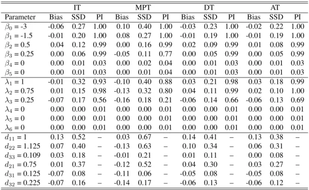
Table 6.1 summarizes the results under the Dirac spike when Sej = 0.95and Spj = 0.98 are

known. The summary includes the empirical bias (Bias), sample standard deviation of the point estimates (SSD), and the average estimated probability of inclusion (PI). Tables 6.12 and 6.13 provide the analogous results under SSVS and NMIG, respectively. These results illustrate that our approach reliably estimates the fixed and random effects; i.e., the empirical bias and the variability of the estimators are small relative to the true value of the corresponding parameter. These results also indicate that the proposed methodology is adept at identifying non-zero fixed and random effects. That is, covariates with strong (no) effects almost always have posterior inclusion probabilities being near 1 (0) in all data sets. Table 6.14 summarizes the results of our ROC analysis. These results show that the average AUC for our model was markedly higher than the competing procedure, across all configurations. This indicates that our approach provides better classification than this existing technique. Further, when comparing Table 6.1 to Tables 6.12 and 6.13, one will note that the Dirac spike tends to outperform both SSVS and NMIG in terms of variable selection.

Among all testing protocols, MPT tends to perform the worst; i.e., the estimates obtained from analyzing MPT data exhibit more bias and variability. This is expected because MPT does not complete classification like the other considered testing protocols; i.e., data collected via MPT consists of less infor-mation about the individuals’ latent statuses when compared to DT, AT, and IT. In contrast, the estiinfor-mation performance under the two classification protocols (DT and AT) is as good if not better than the performance under IT. Keep in mind, these estimates are obtained at nearly half the testing cost on average. Specifically, to complete IT, 5000 tests are used, while DT and AT require on average 2747 and 3258 tests, respectively.

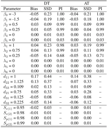
Dirac spike. Under this configuration, the proposed methodology is tasked with estimating four additional parameters through analyzing DT and AT data. Tables 6.15 and 6.16 provide the analogous results under SSVS and NMIG, respectively. These results indicate that the proposed approach can accurately estimate the unknown assay accuracies; i.e., these estimates exhibit little (if any) average bias and the variability in the estimates is small relative to the true value of the testing accuracies. Moreover, there are no appreciable differences between the estimates displayed in Tables 6.1 and 6.2 for DT and AT; i.e., the estimation of the fixed and random effects are not unduly impacted by the additional task of estimating the assay accuracies. It is important to note that flat priors are specified for the testing accuracies in this application to provide for the most challenging case; i.e., we have no prior information about the testing accuracies. In other settings it might be desirable to set informative priors; e.g., if one believes that sensitivity or specificity are around 0.95 an informative prior could be specified as Beta(19c, c), where large(small) values ofc would reflect strong(weak) prior belief. Informative priors could also be designed based on validation trials as we demonstrate in Section 6. In either case, it is reasonable to assume that the proposed methodology would perform as well if not better when informative priors are specified for the testing accuracies.

In addition to the studies described above, we have also performed a complementary study aimed at assessing the robustness of our approach to severe violations of the conditional independence assumption; i.e., the assumption that the testing responses inZare conditionally independent givenZe. Appendix A.2

provides the specific details on how this study was conducted along with a summary discussion of the results. Briefly, this study reveals that the performance of our proposed regression method is not degraded even under severe violations of this assumption.

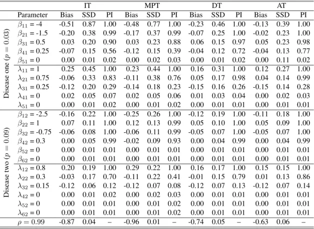
[Table 1 about here.]

[Table 2 about here.]

2.6

Chlamydia testing application

As Iowa’s public health and environmental laboratory, the SHL serves all of the state’s counties through infectious disease detection and surveillance. This includes annually screening thousands of res-idents for the two most common sexually transmitted diseases (STDs): chlamydia and gonorrhea. This process begins with specimens (e.g., urine, swab, etc.) being collected from residents at different clinics (e.g., STD screening clinics, family planning, etc.) throughout the state. These specimens are then

trans-ported to the SHL for testing. Current SHL screening protocols mandate that all male specimens and female urine specimens be tested individually while a variant of Dorfman testing is used to classify female swab specimens; for further discussion, see Tebbs et al. [2013]. The SHL uses the Aptima Combo 2 Assay to test both pooled and individual specimens.

Our analysis focuses on the chlamydia data collected on female patients during the 2014 calendar year. During this time period, 64 different clinics submitted specimens to the SHL for testing. The available data consist of results collected on 4316 individual urine specimens, 416 individual swab specimens, and 2286 swab master pools (1 of size2, 12 of size 3, and 2273 of size4), as well as the test results required to resolve the positive master pools. In addition to the test data, several covariates were collected on each individual: age (in years, denoted byx∗1), a race indicator (x∗2= 1if Caucasian andx∗2= 0otherwise), an indicator denoting

whether the patient reported a new sexual partner in the last 90 days (x∗3 = 1if affirmative and x∗3 = 0

otherwise), an indicator denoting whether the patient reported having multiple sexual partners in the last 90 days (x∗₄= 1if affirmative andx∗₄= 0otherwise), an indicator denoting whether the patient reported sexual contact with an STD-positive partner in the previous year (x∗₅ = 1if affirmative andx∗₅ = 0otherwise), and an indicator denoting whether the patient presented with symptoms (x∗₆ = 1if affirmative andx∗₆ = 0

otherwise). To relate the individuals’ disease statuses to the available covariate information, we assume that g−1_{P(

e

Yi = 1|β,λ,a,bk(i))}=xi0β+t0iΛAbk(i),whereg−1(·)denotes the probit link. The covariate

vectorsxiandtiare taken to be equal and are standardized versions ofxi∗ = (1, x∗i1, x∗i2, x∗i3, x∗i4, xi∗5, x∗i6)0.

This was done so that the spike and slab distributions will have the same impact on the regression coefficients across all covariates. In this analysis, a random effect vectorbk is specified for each of the 64 clinics, with

the convention thatbk(i)=bk if theith individual presented at thekth clinic site.

Given the results of the numerical studies presented in Section 5, in this analysis we chose to imple-ment the proposed approach under the Dirac spike only. All other prior specifications were made in the exact same fashion as was described in Section 5. The only difference being that three sets of testing accuracies were conceptualized to account for the SHL’s screening protocol:Se(1)andSp(1)for swab specimens tested

individually,Se(2)andSp(2)for urine specimens tested individually, andSe(3)andSp(3)for swab specimens

tested in pools. Flat priors were again specified for these parameters; i.e.,Se(m), Sp(m) ∼ Beta(1,1), for

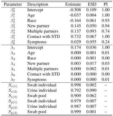
Kuo and Mallick [1998]. The direction (sign) of the point estimates of the fixed effects are congruous with the findings from other similar epidemiological studies involving chlamydia infection. That is, the risk of contracting chlamydia tends to decrease with age, and Caucasians appear to be associated with a lower risk when compared to other races. In contrast, having a new sexual partner, multiple partners, and contact with an STD are all associated with an increased risk. Lastly, our modeling framework identified the random intercept parameter to be strongly significant; i.e., there exists strong evidence of heterogeneity across the various clinics throughout the state. It is worthwhile to point out that these random intercepts act as crude proxies for clinic level unmeasured confounders such as an areas socioeconomic status, rural verses urban areas, etc. By examining these estimated random effects alongside other predictor variables (e.g., census data) one could reveal new covariates that are related to chlamydia prevalence.

Shifting attention to the estimates of the testing assay accuracies, one may notice the lower estimates ofSe(2) andSe(3), suggesting potential underestimation of these parameters. To examine this further, we

performed the analysis again using informative priors which were set based on the product literature and validation trials available on the Aptima Combo 2 Assay; see McMahan et al. [2017]. A summary of the results is provided in Table 6.17. From these results, one will note that there are no appreciable differences in the regression parameter estimates. Therefore, even if the testing accuracies are slightly underestimated, this does not appear to unduly affect the estimation of the regression parameters, which are likely of primary interest. When comparing Table 6.3 to Table 6.17, we find evidence that all testing accuracies are identifiable under the Iowa testing protocol, withSe(2)andSe(3)being weaker “learners” thanSe(1). This feature is likely

attributable to the specified testing protocol; e.g., testing all female urine specimens individually provides very little confirmatory and/or counter-factual information that can be used to estimateSe(2).

Lastly, based on our posterior sampling strategy we are able to estimate a subject specific posterior infection probability for each individual given all of the observed data. This is accomplished by averaging over the sampled latent statuses for theith individual; i.e., we compute the subject specific posterior infection probability as G−1PG

g=1Ye (g)

i , whereYe (g)

i is thegth posterior draw ofYei, forg = 1, ..., G. Figure 6.6

displays these posterior probabilities for the individuals in this study, stratified by diagnosed status. These probabilities can be used as a measure of diagnostic certainty; e.g., probabilities near 1(0) indicate that the individual is (not) infected. Further, we believe that these probabilities could also be used to guide back-end confirmatory screening via informative group testing procedures; e.g., see McMahan et al. [2012] and Bilder et al. [2019].

[Table 3 about here.]

2.7

Discussion

This work has developed a Bayesian generalized linear mixed model that can be used to analyze data arising from any group testing protocol. To further disseminate our work, R programs which implement the proposed approach have been developed and are available at

www.chrisbilder.com/grouptestingand a description of the main functions can be found in Ap-pendix A.3.

Given the performance of the proposed approach, several modeling extensions could be of inter-est. For example, many large-scale screening laboratories are now adoptingmultiplex assays, which test specimens for multiple diseases simultaneously. That is, a multiplex assay generates a multivariate outcome consisting of correlated binary data. Extending the proposed modeling framework to account for this type of data would be of interest. Further, the proposed methodology could also be generalized to an additive model framework with variable selection being applied to nonlinear functionals of the continuous predictors.

Chapter 3

Mixed effects Bayesian regression for

multivariate group testing data

3.1

Introduction

Group testing has received a considerable amount of attention in recent years; rightfully so as it has the potential to save practitioners a considerable amount of money in testing costs. In its essence, a group testing protocol reduces the total number of tests required to screen a population for an infectious disease. This phenomenon was first well established by Robert Dorfman in 1943 when he proposed his Dorfman group testing algorithm to test United States soldiers for syphilis during World War II. Individuals were placed into groups where their specimens (e.g., blood, urine, swabs, etc) were physically combined into a pool. That pool is then tested for an infectious agent at the expense of a single diagnostic assay. Group testing protocols proceed in the following manner: If the pooled specimen tests negatively, then all individuals are declared disease free, and contrastly, if a pool tests positively, contributing members are then retested algorithmicially to determine which individuals are positive. Today, the State Hygienic Laboratory (SHL) in Iowa currently employs a group testing protocol and has reported a $3.1 million savings over a course of 5 years after adopting the Dorfman group testing algorithm as their primary testing protocol. Pooling biospecimens through group testing arises in many applications, including testing for HIV, HBV, and HCV [Kleinman et al., 2005, Sarov et al., 2007, Krajden et al., 2014], testing animal and insect populations [Dhand et al., 2010, Speybroeck et al., 2012], environmental testing [Heffernan et al., 2014], and drug discovery

[Hughes-Oliver, 2006].

The group testing literature has grown vastly in recent years due to the dramatic cost effectiveness that group testing offers over individual level testing. To name a few, some of the more recent notable works include Vansteelandt et al. [2000], Bilder and Tebbs [2009], Delaigle and Meister [2011], and McMahan et al. [2017]. However, these methods analyze data from a group testing algorithm through a univariate analysis; i.e., to model data from a group testing protocol that used multiplex testing assays, they would have to perform multiple univariate analyses. However, this practice may miss important features in the data, such as correlation between diseases. That is, an individual who has disease one may be more likely to have disease two. However, to date, there is a lack of existing methodology in the group testing literature to perform a multivariate analysis of group testing data where a multiplex testing assay was used.

To further the model complexity, most public health laboratories like the SHL receive individual specimens from different clinics. Given the different types of clinics (e.g., family planning clinics, STD testing clinics, etc.) and different locations of clinics (e.g., urban area versus rural), it is reasonable to believe that heterogeneity may exist from clinic to clinic. However, like the SHL, most laboratories pool individual specimens as they arrive. That is, contributing members may share different clinic effects. This provides for a challenging modeling framework.

In this paper, we develop a general multivariate Bayesian generalized linear mixed effects model to analyze data arising from any group testing protocol. That is, individuals may be pooled together and restested in any fashion, and may be tested for more than one disease simultaneously. The novelty of this methodology is the multivariate analysis of such data, and furthermore, we achieve full model selection via spike and slab priors.

The remainder of this paper is organized as follows. Section 2 introduces the notation seen through-out this manuscript and lays through-out the developed methodology. Section 3 assesses the models capability of estimating the unknown parameters for a given group testing data set. Section 4 analyzes the motivating group testing data set, provided by the State Hygienic Laboratory (SHL) in Iowa. Finally, Section 5 con-cludes the manuscript with a brief discussion.

3.2

Methodology

3.2.1

Notation and preliminaries

Suppose that there areN individuals who are tested for the presence of any ofDdiseases through a group testing procedure that used a multiplex testing assay. These individuals each visit one ofKdistinct clinics, where an individual’s specimen (e.g., blood, urine, swabs, etc) is extracted for evaluation. These specimens are either tested in house at the clinic site or sent to a central hub for testing; e.g., the State Hygienic Laboratory in Iowa. In either case, the testing is done by formingJ total groups (pools), where the jth pool involvescj individuals; i.e., N = P

J

j=1cj. For the methodology to incorporate data from

any group testing algorithm, definePj to be the set of individuals involved in thejth pool. Regardless of

the group testing algorithm, keeping track of pool membership will suffice for model fitting. Let the true status of individual i = 1,2, ..., N beYei = (Yei1, ...,YeiD)0, a D dimensional binary vector, and the true

status of poolj = 1,2, ..., J beZej = (Zej1, ...,ZejD)0, also aD dimensional binary vector. Here,Yeid = 1

(Yeid = 0)if individualiis truly positive (negative) for thedth disease. Group testing protocols mandate that

a pool is positive if at least one member is truly positive; i.e.,Zejd = max{Yeid : i ∈ Pj}. Unfortunately,

these binary vectors are never truly known due to testing assays of any kind being subject to error; i.e., false positives or false negatives. To this end, denote the observed diagnoses asYi = (Yi1, ..., YiD)0andZj =

(Zj1, ..., ZjD)0. Moreover, to acknowledge these imperfect testing assays, each pool receives a sensitivity

Sej = (Sej:1, ..., Sej:D)0 and specificitySpj = (Spj:1, ..., Spj:D)0, whereSej:d =P(Zjd = 1| Zejd = 1)

andSpj:d =P(Zjd= 0|Zejd= 0). The testing assay accuracies may be known constants and provided to

the model, or the model can simultaneously estimate them during model fitting; more details in Section 3.2.4. To address the possible heterogenity that may exist across the clinic sites, a mixed effects model is used to relate an individual’s covariate information to their infectious probability. For each of theKclinics, thekth site gets assigned a random effect vectorγkd, which is assumed to be a multivariate normal random

vector with mean zero and covariance matrixΣd, i.e.,γkd∼N(0,Σd). Define for individualiand disease

d,xidas thepddimensional covariate vector associated with the fixed effects andtidas theqddimensional

covariate vector associated with the random effects. Letβdandγkdbe the unknown fixed and random effects

vectors for the dth disease, respectively. It is assumed that the random effects are pairwise independent across all sites and all diseases, i.e., γkd is independent of γk0_d0 for all k, d 6= k0, d0. For individuali, we setγ(i)d = γkd if and only if individuali was a patient at thekth clinic site. For ease of notation,

aggregateβ= (β0₁, ...,β_D0 )0, ap=PD d=1pddimensional vector,γ(i)= (γ(0i)1, ...,γ 0 (i)D) 0_{, aq=}PD d=1qd

dimensional vector,Xi=diag(x0i1, ...,x0iD), aD×pcovariate matrix associated with the fixed effects, and

Ti=diag(t0i1, ...,t0iD), aD×qdimensional covariate matrix associated with the random effects. Then, the

multivariate infectious probability of theith individual is related to their covariate information through the following multivariate generalized linear mixed model

P(Yei =y_ei |β,γ(i),θ) =g(ηi;θ) (3.1)

wheregis a known multivariate link function,θis a collection of link dependent parameters (e.g., a correla-tion matrix in the multivariate probit link) andηi= (ηi1, ..., ηiD)0, whereηid =x0idβd+t0idγ(i)d.

Mixed effects models are important for clustered observations (clinics), but the dimension of free parameters quickly becomes an issue and furthermore, the prior specification of each covariance matrixΣd

may not be clear. To overcome these challenges, Chen and Dunson [2003] propose reparameterizatizing the covariance matrices as Σd = ΛdAd0AdΛd via a modified Cholesky decomposition. Here, Λd is a

nonnegativeqd dimensional diagonal matrix with entriesλd andAd is aqd ×qd lower triangular matrix

with entries ad = (amld: l = 1, ..., qd −1;m = l + 1, ..., qd)0 and unit main diagonal. Aggregating λ= (λ0₁, ...,λ0_D)0anda= (a0₁, ...,a0_D)0, the reparameterized model is

P(Yei=yei|β,λ,a,b(i),θ) =g(ηi;θ) (3.2)

where nowηid =x0idβd+t0idΛdAdb(i)d, andb(i)dis the standardized clinic specific random effect

asso-ciated with thedth disease. Specifically,bkd ∼N(0,I)andb(i)d =bkdif and only if theith individual’s

specimen was extracted at thekth clinic. Here, the standardized random effects adopt the same assumptions as the original random effects. The benefit of model (3.2) over the unparameterized model is twofold. First, it is no longer necessary to specify, or posit prior structure on, the covariance matricesΣd,d= 1, ..., D; instead

they are estimated throughΛdandAd. Second, by setting a diagonal element ofΛdto zero effectively zeros

out the corresponding row and column ofΣd, rendering that random effect insignificant. To this end, a spike

and slab prior distribution is utilized to exploit this feature, facilitating variable selection in both the fixed effects and random effects.

the relationship of the group testing data to the individual level model expressed in (3.2), which is given by π(Z|β,λ,a,b,θ) =X    D Y d=1 J Y j=1 n S_eZjd j:d(1−Sej:d) 1−ZjdoZejdn S_p1−Zjd j:d (1−Spj:d) Zjdo1−Zejd × N Y i=1 P(Yei=eyi|β,λ,a,b(i),θ) ) , (3.3)

whereb= (b1, ...,bK)0. Note that in expressing this conditional distribution, a few mild assumptions have

been made. First, it is assumed that the testing outcomes for each disease are conditionally independent given the true pool statusesZe (i.e.,Zjd|Ze is independent ofZj0_d0 |Ze) and that the conditional distributionZ|Ze

does not depend on the individuals’ covariates. Second, the individuals’ true statusesYeiare conditionally

independent given the covariates and the random effects. To proceed, note that the summation in (3.3) is over all possibleD dimensional binary true statuses for allN individuals, rendering direct evaluation infeasible. To overcome this, we utilize a data augmentation strategy used in error prone group testing literature; see McMahan et al. [2017]. By introducing the true latent statusesYeias random variables, we instead consider

the joint conditional distribution

π(Z,Ye |β,λ,a,b,θ) = D Y d=1 J Y j=1 n SZjd ej:d(1−Sej:d)1−Zjd oZjde n S1−Zjd pj:d (1−Spj:d)Zjd o1−Zjde × N Y i=1 P(Yei=yei|β,λ,a,b(i),θ). (3.4)

whereYe = (Ye₁0, ...,Ye0_N)0. It should be noted that this data augmentation strategy will require sampling the