Self-Referential Options

(1)

Self-Referential Options

Candidate Number: 761637

St Cross College

University of Oxford

A thesis submitted for the degree of

MSc Mathematical and Computational Finance

June 25, 2015

Manjae Han

(2)

Acknowledgements

Firstly, I praise to God Almighty for leading my way with His endless mercy and blessings.

I would like to pass on my gratitude to my supervisor Prof Howison for not only the guidance and support he has given me but also for granting me a great opportunity to work on an interesting project. I would also like to thank Dr Dewynne who offered the project in the first place but was unfortunately unable to supervise due to personal matters. Last but not least, I would like to thank Prof Cohen for giving great lectures on Exotic options which took essential roles in writing the thesis.

(3)

Abstract

This thesis mainly focuses on various types of exotic option contracts with special feature, namely self-referential property. An exotic option is defined to be self-referential if one of its parameters (e.g. strike, bar-rier) reflects the option value and, hence, the option price itself affects the evolution of the option price. Self-referential versions of forward-start options, barrier options and Asian options will only be concerned in this thesis. Self-referential option prices are not always well-defined or stable. In fact, such options do not even exist for certain type of exotic options with certain conditions on their parameters. Therefore, under the stan-dard Black-Scholes market assumption, we are going to price such options and study existence and stability of price functions.

(4)

Chapter 1 Introduction

The thesis is mainly concerned with options whose price influences their own evolu-tion through a feedback mechanism, for example carbon allowance prices where the feedback is via the dependence of prices on emissions and emissions on prices.

1.1 Market definition

We will build pricing models in a standard complete Black-Scholes market with a risk-free asset and a risky asset. The definition of the Black-Scholes market follows from [1]. The Black-Scholes market assumes that trading is frictionless, market ran-domness is described by a standard Brownian motion{Wt}t≥0 in a probability space

(Ω,F,_P;{Ft}t≥0), and the filtration {Ft}t≥0 is market information which contains

historical randomness up to time t. We further assume that the risky asset {St}t≥0

and risk-free asset{Bt}t≥0 follow the dynamics

dSt St = (µ−q)dt+σdWt, dBt Bt =rdt,

whereµ is the growth rate, r is the interest rate, q is the dividend rate, and σ is the volatility. Moreover, anyFT-measurable contingent claim paid at timeT is replicable

due to the complete market assumption.

If we also assume the Markov property of the price process Vt of any replicable

contingent claim, then we can writeVt as a function oft and S only,

Vt=V(t, St).

Portfolio replication shows that the price process satisfies the Black-Scholes PDE,

∂V ∂t + 1 2σ 2_S2∂2V ∂S2 + (r−q)S ∂V ∂S −rV = 0, V(T, S) = Ψ(S), (1.1.1)

(7)

where Ψ(·) is the payoff function of the contingent claim at the maturity T.

Solving (1.1.1) with payoff Ψ(S) = max{S−K,0} and max{K−S,0} gives the Black-Scholes price functions of European call and put options,

CBS(t, S;K, T) =S e−q(T−t)N(d+)−K e−r(T−t)N(d−),

PBS(t, S;K, T) =K e−r(T−t)N(−d−)−S e−q(T−t)N(−d+),

whereK is the strike, d± are defined by

d±=

log(S/K) + (r−q± 1 2σ

2₎₍_T ₋_t₎

σ√T −t , (1.1.2)

and N(·) is the cumulative normal distribution function,

N(x) = √1 2π x Z −∞ e−z2/2dz.

1.2 Motivation and application to carbon markets

We look for the motivation of self-referential options in the carbon market model and the following definitions and problem formulation are from [3] and [4].

In order to mitigate the greenhouse effect, countries are agreed by Kyoto Protocol, 1992, to reduce the carbon emissions and set a quantitative limit or cap on the amount of emissions of a pollutant. As an effective way of meeting the obligations, allowance certificates are introduced and carbon markets are set up for the purpose of controlling the carbon emissions. Allowance certificates are freely tradable products which provide the right to emit one unit of pollutants. Moreover, allowance certificates are created equal to the cap in quantity. In the carbon market, polluters have to either pay the fixed rate penalty or produce an allowance certificate according to the amount of carbon they emitted at the end of the set period. Hence there may be an incentive for producers to sell allowances if they are under-emitting and do not need their quota, or to buy them if they are likely to over-emit and it is expected to be cheaper to do this than pay the penalty. Producers can also switch to expensive but clean fuel if the allowance price is large. We model this by first introducing an exogenous stochastic process Dt which corresponds to the demand of allowance in the carbon

market. We assume that the demand process Dt satisfies the dynamics

dDt=µDdt+σDdWtQ

under the risk-neutral measure Q. The demand drives the production and therefore it affects the emission rate. So we letAt be a risk-neutral price process of allowance

and assume that the emission rateet is a function ofDt andAt. The assumption can

(8)

before the carbon emissions. Intuitively,et(At, Dt) is decreasing in At and increasing

inDt. With the emission rate given, we have the total emissions as

Et = t

Z

0

es(As, Ds)ds.

Then the dynamics ofEt is

dEt=e(At, Dt)dt.

Note that the determination of et is previsible and hence the process Et is also

pre-visible. Now considerAt as a function of Dt and Et,

At=A(t, Dt, Et),

then by Itˆo’s lemma,

d e−rtAt =e−rt ∂A ∂tdt−rAdt+ ∂A ∂DdDt+ 1 2σ 2 D ∂2_A ∂D2dt+ ∂A ∂EdEt =e−rt ∂A ∂t + 1 2σ 2 D ∂2_A ∂D2 +µD ∂A ∂D +e(A, D) ∂A ∂E −rA dt+σD ∂A ∂DdW Q t .

SinceAtis a tradable asset, discounted allowance price under the risk-neutral measure

Q is a martingale. So equating the drift term to zero will give a nonlinear partial differential equation thatA(t, D, E) satisfies:

∂A ∂t + 1 2σ 2 D ∂2A ∂D2 +µD ∂A ∂D +e(A, D) ∂A ∂E −rA= 0.

The PDE we obtained from the model of the allowance price is similar to the Black-Scholes PDE apart from the nonlinear term. We note that the PDE is nonlinear since the allowance price affects its own evolution through e(A, D).

Self-referential options share the same features with the carbon market model in the sense that the option value itself affects the evolution of the price process. Hence we discuss a few different self-referential versions of exotic options as simplified examples of the carbon market model.

(9)

Chapter 2 Self-referential forward-start

options

In this chapter, we follow the second chapter of [2] to formulate the problem and extend the idea to discuss the stability of option prices. We start with the brief study of pricing standard start options. Then we define a self-referential forward-start option as a forward-forward-start option whose strike is determined by the time-T1option

value itself, rather than the value of the underlying risky asset. So at some time T1

before the maturity, the strike will be defined as

K =α V(T1, S;α),

where α is some positive constant and V(·) is a price function of the self-referential forward-start option. For time T1 < t≤T, the strike and payoff are known and the

option price could be derived by solving the Black-Scholes equation, i.e. the option price is equal to the standard Black-Scholes price function for European options. Then we claim the continuity of the price function at t = T1 and the problem will

essentially reduce down to a transcendental equation of the form

K =α VBS(T1, S;K, T). (2.0.1)

We first analyse the existence of solution of the transcendental equation. It is possible for the equation to have a unique root, no root at all or more than one root. The number of different roots of the equation represents the possible self-referential option contracts with different strikes. Hence the price of the self-referential forward-start option is only defined when there exist roots of the transcendental equation and only well-defined if there is a unique root. Note also that for given α the root of the transcendental equation (2.0.1) will be different in general for call and put options. This implies that the put-call parity is not available for the self-referential forward-start options. Although the existence or the number of roots will be discussed, the roots will not be derived explicitly. It is expected to be computed numerically by using the Newton’s iteration or bisection method.

We will end the chapter with discussion about the stability of the roots of the transcendental equation. When the option value in the equation is perturbed, the

(10)

root of the equation is defined to be stable if the perturbation converges to zero. Stability condition will be derived and applied to different price functions.

2.1 Standard forward-start options

A standard forward-start option is a European option which starts at a specified future date and expires at some later time in the future after it starts. We will consider the case that when the option starts, the strike is determined according to the underlying asset value at that time. We assume that the option expires atT, and strike K will be determined at T1 ≤T as

K =αST1,

for some constant α > 0. Since ST1 is Ft-measurable for t ∈ [T1, T], the strike of the option is deterministic for t ≥ T1. Hence, the option value is equal to the

corresponding standard European option price

V(t, S;α) =VBS(t, S;αST1, T).

Att=T1, applying the Black-Scholes price function of European call option gives

CBS(T1, ST1;αST1, T) = ST1 e −qτ N(dα₊)−αST1 e −rτ N(dα₋) = e−qτN(dα₊)−α e−rτN(dα₋)ST1 =AC(τ, α)ST1 whereτ =T −T1 and dα_± = −log(α) + (r−q± 1 2σ 2₎_τ σ√τ .

SinceAC(τ, α) is deterministic for all time, one can replicate the payoffAC(τ, α)ST1 at time T1 with AC(τ, α)Ste−q(T1−t) at timet ∈[0, T1]. Therefore, the price of standard

forward-start call is C(t, S;α) =      CBS(t, S;αST1, T) for T1 ≤t ≤T, AC(τ, α)S e−q(T1−t) for 0≤t≤T1, where AC(τ, α) = e−qτN(dα+)−α e −rτ N(dα₋).

Similarly, the forward-start put price is

P(t, S;α) =      PBS(t, S;αST1, T) for T1 ≤t≤T, AP(τ, α)S e−q(T1−t) for 0≤t≤T1,

(11)

ξ

c

(

τ

,

α

)

1 α

C

B S

(

ξ

)

ξ

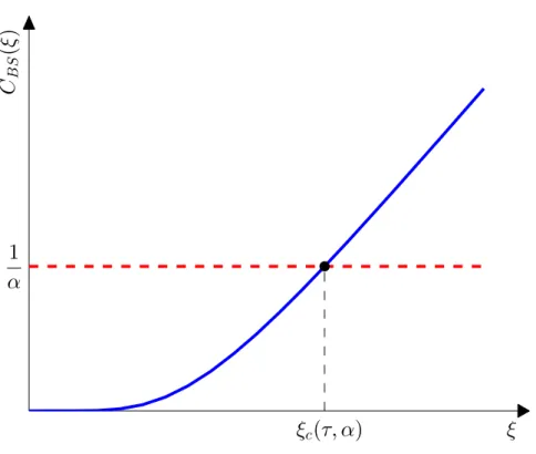
Figure 2.1: The solution ξc(τ, α) of CBS(T1, ξ; 1, T) = 1/αfor τ > 0 andα >0.

where

AP(τ, α) = α e−rτN(−dα−)−e −qτ

N(−dα₊).

2.2 Self-referential forward-start call

2.2.1 Option pricing with a transcendental equation

For the case of a self-referential forward-start call, we define that the strike is set at time T1 < T according to the option value C(·) as

K =α C(T1, S;α)

for some constant α > 0. For times t ∈ (T1, T], the strike is deterministic and the

option is exactly the same as a standard European call option. No-arbitrage implies continuity of C(t, S;α) at t=T1 and this gives

C(T1, S;α) = CBS(T1, S;K, T).

Therefore, we have a transcendental equation forK:

(12)

If there exists a solution to the transcendental equation (2.2.2) for K, the value of the option for t ∈ [T1, T] will be determined by the standard Black-Scholes price of

European call with strikeK, which is the root of the equation.

To see the existence of solution of (2.2.2), recall the call price function and in-troduce a new variable ξ = S/K. Rearranging the equation (2.2.2) in terms of ξ

gives 1 = α KCBS(T1, S;K, T) = α K S e −q(T−T1)_N₍_d +)−K e−r(T−T1)N(d−) =α ξ e−q(T−T1)_N₍_d +)−e−r(T−T1)N(d−) =α CBS(T1, ξ; 1, T), where d±= log(S/K) + (r−q± 1 2σ 2₎₍_T ₋_T 1) σ√T −T1 = log(ξ) + (r−q± 1 2σ 2₎₍_T ₋_T 1) σ√T −T1 . (2.2.3)

Hence, the equation (2.2.2) becomes

CBS(T1, ξ; 1, T) =

1

α, (2.2.4)

and note that lim

ξ→0CBS(T1, ξ; 1, T) = 0 and ξ→∞lim CBS(T1, ξ; 1, T) =∞.

SinceCBS(T1, ξ; 1, T) is a strictly increasing function ofξwhich starts from 0 at ξ= 0

and goes to infinity as ξ → ∞, there exists a unique ξ satisfying (2.2.4). Figure 2.1 shows the root. Moreover, suchξ only depends on the constant α and the remaining time until expiry. So we can write the unique root of (2.2.4) as a function of α and

τ =T −T1 only:

ξ=ξ_c∗(τ, α).

In order to get the option value for t∈[0, T1], consider

K∗(τ, α, S) = ST1

ξ∗ c(τ, α)

and the option value atT1 satisfies

C(T1, S;α) = K∗(τ, α, S) α = ST1 αξ∗ c(τ, α) .

(13)

Since C(t, S;α) satisfies the Black-Scholes PDE and α ξ∗_c(τ, α) is deterministic, one can replicate time t price of the option by directly discounting the T1-price with

dividend rate. Thus, the self-referential forward-start call option value is

C(t, S;α) =            CBS t, S; ST1 ξ∗ c(τ, α) , T for T1 ≤t ≤T, S e−q(T1−t) α ξ∗ c(τ, α) for 0≤t < T1,

whereξ_c∗(τ, α) is the unique solution of (2.2.4).

2.2.2 Stability of the solution of forward-start call options

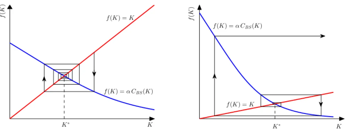
We now analyse the stability of the transcendental equation (2.2.2). For simplicity of notation, write the transcendental equation as

ξ=f(ξ). (2.2.5)

If we force up the call option price prior to T1 for fixed α, the strike will rise

conse-quently. Increasing the strike will decrease the call price and the effect of forcing up the option price offsets this. Mathematically, the root is defined to be stable if the sequence{n}n∈_N satisfying the iteration

ξ∗+n+1 =f(ξ∗+n) (2.2.6)

converges to zero, where 0 is small (as defined below) and ξ∗ is a root of the

tran-scendental equation (2.2.5). Taylor expanding (2.2.6) gives

ξ∗+n+1 =f(ξ∗) +f0(ξ∗)n+

1 2f

00

(ξ∗)2_n+O(3_n) and useξ∗ =f(ξ∗) to get

n+1 =a n+b 2n

where

a=f0(ξ∗), b= 1 2f

00_{( ˆ}_ξ₎

for some ξ∗ ≤ ξˆ ≤ ξ∗ +n. For all sufficiently small n we assume that f00(ξ) is

bounded by 2b for all ξ ∈ [ξ∗, ξ∗ +n]. Suppose |n| < ∗ for some ∗ > 0 then the

following holds: |n+1| ≤ |a||n| 1 + b an <|a||n| 1 + |b| |a| ∗ . (2.2.7)

If|a|<1, we can choose ∗ such that

c=|a| 1 + |b| |a| ∗ <1,

(14)

K K∗ f(K) =K f(K) =αCBS(K) f ( K ) K K∗ f(K) =K f(K) =αCBS(K) f ( K )

Figure 2.2: Stability graphs of the iteration (2.2.6) for self-referential forward-start call options. The left-hand side is the case of stable solution (α < α∗_s) and the right-hand side is unstable solution(α≥α∗_s).

which gives the condition on ∗,

∗ < 1− |a|

|b| .

Then (2.2.7) implies that

|n+1| ≤c|n|,

where 0 < c < 1 and this shows that {n}n∈_N is a decreasing sequence with lower

bound at zero. Hence, the sequence converges to zero and the solution also converges to the real root ξ∗. This implies that the solution of the transcendental equation is stable if the stability condition

|f0(ξ∗)|<1 (2.2.8) is satisfied and any ξ with |ξ∗ −ξ| < ∗ converges to the actual solution. For small enough 0, this is if and only if condition condition. But, to be precise, we say that

the stability is not guaranteed if the solution does not satisfy (2.2.8). Now we check the condition for this problem. First, compute

∂ ∂KCBS(T1, S;K, T) = ∂ ∂K S e −qτ N(d+)−K e−rτN(d−) = S e−qτN0(d+)−K e−rτN0(d−) ∂d ∂K −e −rτ N(d−), where ∂d± ∂K = ∂d ∂K =− 1 σK√τ.

Using the identityS e−qτN0(d+) =K e−rτN0(d−),

∂

∂KCBS(T1, S;K, T) = −e

−rτ

(15)

Since the function we are considering here is α CBS(T1, S;K, T), we obtain the

sta-bility condition on α for the root of (2.2.2) by using (2.2.8),

α < α_s∗ = 1

e−rτ_N₍_d −)

.

2.3 Self-referential forward-start put

2.3.1 Option pricing with a transcendental equation

With the similar approach as above, we assume that the strike is set at time T1 < T

as

K =α P(T1, S;α)

for some constant α >0. Likewise, by no-arbitrage and continuity of price function, a transcendental equation could be derived

K =α PBS(T1, S;K, T). (2.3.9)

Since PBS(T1, S; 0, T) = 0, there is a trivial solution, K = 0. In the case of trivial

solution, the option is worthless throughout whole time period fromT1 toT. In order

to verify the existence of non-trivial solutions, we write out the Black-Scholes price function for European put options in terms ofξ =S/K

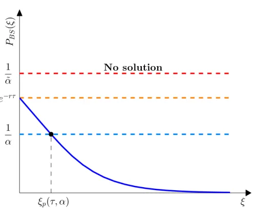
1 = α KPBS(T1, S;K, T) = α K K e −r(T−T1)_N₍₋_d −)−S e−q(T−T1)N(−d+) =α e−r(T−T1)_N₍₋_d −)−ξ e−q(T−T1)N(−d+) =α PBS(T1, ξ; 1, T) ≤α PBS(T1,0; 1, T) =α e−r(T−T1)

where d± is the same as (2.2.3). We obtained the condition for the existence of the

non-trivial solutions as

α≥α∗ =erτ, (2.3.10)

whereτ =T−T1. Forα satisfying (2.3.10), write the transcendental equation (2.3.9)

as an equation ofξ only,

PBS(T1, ξ; 1, T) =

1

α, (2.3.11)

and note that

lim

ξ→∞PBS(T1, ξ; 1, T) = 0.

Since (2.3.10) is satisfied and PBS(T1, ξ; 1, T) is a strictly decreasing function of ξ

(16)

ξ

p

(

τ

,

α

)

1 α

e

−rτ

1 ˜

α

P

B S

(

ξ

)

ξ

No solution

Figure 2.3: The solution ξp(τ, α) of PBS(T1, ξ; 1, T) = 1/α for α > α∗, α = α∗, and

α= ˜α < α∗, whereα∗ =erτ.

Suppose the unique solution of (2.3.11) is given by

ξ=ξ_p∗(τ, α).

Then the self-referential forward-start put becomes a standard European put with strike K∗(τ, α, S) = ST1/ξ

∗

p(τ, α) for timet ∈[T1, T]. At time T1,

P(T1, S;α) = K∗(τ, α, S) α = ST1 αξ∗ p(τ, α) ,

and the same argument as the case of call options gives the price function of the self-referential forward-start put option,

P(t, S;α) =              PBS t, S; ST1 ξ∗ p(τ, α) , T for T1 ≤t≤T, S e−q(T1−t) α ξ∗ p(τ, α) for 0≤t≤T1,

(17)

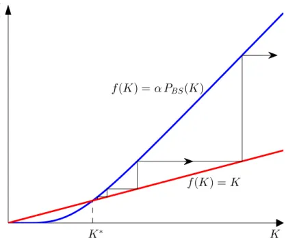
K K∗ f(K) =K f(K) =αP_BS(K) f ( K )

Figure 2.4: Stability graph for self-referential forward-start put options. The graph shows the iteration of an unstable solution.

2.3.2 Stability of the solution of forward-start put options

Forcing up the put option value will increase the strike in the transcendental equa-tion (2.3.9). This will result in the further increase in the put price. So the initial perturbation will grow through the iteration and this will cause the solution of the transcendental equation to explode. Thus the solution is expected to be unstable. We check the stability condition (2.2.8) again with the Black-Scholes price function of European put option.

We compute the first K-derivative of the Black-Scholes price function,

∂ ∂KPBS(T1, S;K, T) = ∂ ∂K K e −rτ_N₍₋_d −)−S e−qτN(−d+) =e−rτN(−d−)− ∂d ∂K K e −rτ N0(−d−)−S e−qτN0(−d+) .

Noting that N0(−d±) = N0(d±) and using the identity S e−qτN0(d+) = K e−rτN0(d−)

again to get ∂ ∂KPBS(T1, S;K, T) =e −rτ_N₍₋_d −). Note that ∂ ∂KPBS(T1, S;K, T) K=0 = 0

(18)

solution to be stable, we require

α < 1 e−rτ_N₍₋_d

−)

.

But since S e−qτN(−d+)>0, we have

α= K ∗ PBS(T1, S;K∗, T) = K ∗ K∗_e−rτ_N₍₋_d −)−S e−qτN(−d+) > K ∗ K∗_e−rτ_N₍₋_d −) = 1 e−rτ_N₍₋_d −) .

Therefore, as we expected, there is noαvalue at which the root of the transcendental equation (2.3.9) is guaranteed to be stable.

(19)

Chapter 3 Self-referential barrier options

In this chapter, we are going to first introduce standard barrier options briefly and build up the problem to the self-referential versions of barrier options. The method of pricing standard barrier options follows from [6] and [7] and all the materials on self-referential options in this chapter is new. Then we will mainly discuss the existence and stability of the solution of self-referential down-and-out and down-and-in calls and puts. We define self-referential barrier options as barrier options whose barrier initially reflects the value of the option itself. So we have

B =β VBarrier(0, S0;K, T, B), (3.0.1)

for some constantβ >0 andVBarrier(·) is the price function of corresponding standard

barrier option. The problem again reduces down to solve a transcendental equation. Likewise, the problem is only well-defined when there exists a unique root to the transcendental equation. The stability of the solution follows in the same sense as the case of self-referential forward-start options. We also note that the standard result of barrier options such as the out-in-parity does not hold for the self-referential barrier options. This is because for givenβ, the root to the transcendental equation (3.0.1) is generally different for down-and-out and down-and-in options. Trivially sum of down-and-out and down-and-in options with different barriers is not equal to a European option.

To simplify the calculations, we further assume that the dividend rate q is zero and omit the analysis of the up-and-out and up-and-in options since the parallel result holds as down-and-out and down-and-in options.

3.1 Standard barrier options

A typical barrier option is an option contract which is activated or knocked out if the underlying asset hits a specified level, the barrier. There are four main different types of barrier options:

• Down-and-out: The underlying price starts above the barrier. The option will be knocked out if the underlying hits the barrier.

(20)

• Up-and-out: The underlying price starts below the barrier. The option will be knocked out if the underlying hits the barrier.

• Down-and-in: The underlying price starts above the barrier. The option will be activated if the underlying hits the barrier.

• Up-and-in: The underlying price starts below the barrier. The option will be activated if the underlying hits the barrier.

Price functions of the four types of barrier put and call options can be found in Ap-pendix A. Standard way of pricing barrier options follows by introducing a reflection term W(t, S) = S B 2α V t,B 2 S . (3.1.2)

where α = 1₂ −r/σ2_{. Note that (3.1.2) satisfies the Black-Scholes PDE and clearly}

the linear combination of the value function V(S, t) and the reflection term W(S, t) also satisfies the Black-Scholes PDE. There are two more conditions to be considered:

i) the same payoff at the maturity,

ii) the option value equal to zero at the barrer.

Since the Black-Scholes PDE is linear, the solution is unique. Hence if all the condi-tions are satisfied, the linear combination is indeed the price of the barrier option.

We take a down-and-out call option as an example. Consider the following for

S > B as a price function of a down-and-out call option and check the conditions,

CDO(t, S;K, T, B) =                    CBS(t, S;K, T)− _BS 2α CBS t,B_S2;K, T for 0≤B < K, CBS(t, S;B, T) + (B −K)Cd(t, S;B, T) − S B 2α CBS t,B_S2;B, T for K ≤B, −(B −K) S_B2αCd t,B_S2;B, T (3.1.3) whereCd(·) is a Black-Scholes price function for a digital call option satisfying

Cd(t, S;K, T) = e−r(T−t)N(d−),

with d− is defined the same as (1.1.2). Since CBS(·) and Cd(·) satisfy the

Black-Scholes PDE, so does (3.1.3). Note that we also have CDO(t, B;K, T, B) equal to

zero for both 0 ≤ B < K and K ≤ B, and this shows that the barrier condition is satisfied. Lastly, in order to achieve the call payoff, consider cases separately,

(i) If 0 ≤ B < K and S > B, then 0 < 1/S < 1/B. Multiplying by B2 gives

B2_{/S < B < K}_{. Then the payoff of the reflection term is} S B 2α CBS T,B 2 S ;K, T = S B 2α max B2 S −K,0 = 0.

(21)

Hence, we recover the call payoff if the option survived until the maturity. (ii) If K ≤B and S > B, then

Cd(T, S;B, T) = 1{S>B} = 1, Cd T,B 2 S ;B, T =1n B2 S >B o =1_{B>S} = 0, CBS(T, S;B, T) = max{S−B,0}=S−B, CBS T,B 2 S ;B, T = max B2 S −B,0 = 0.

We recover the call payoff again.

Therefore, the payoff of the survived option is the same with the call payoff and

CDO(t, S;K, T, B) is indeed the price function of down-and-out call option.

3.2 Self-referential down-and-out options

We define a self-referential down-and-out option as an option contract which keeps all the features of a standard down-and-out option and its barrier is determined at time zero to reflect the option price itself. We assume that the barrier takes the form

B =β VDO(0, S0;K, T, B), (3.2.4)

for some constant β > 0. Similar to the self-referential forward-start options, the problem reduces down to solve a transcendental equation forB.

3.2.1 Self-referential down-and-out call options

We define the barrier of a self-referential down-and-out call option as

B =β CDO(0, S0;K, T, B), (3.2.5)

for some constantβ >0. First, note that CDO(0, S0;K, T, B) is a strictly decreasing

function ofB. We also have limits lim

B→SCDO(0, S0;K, T, B) = 0,

lim

B→0CDO(0, S0;K, T, B) =CBS(0, S0;K, T)>0.

The down-and-out call price function (3.1.3) is continuous at B =K with the value

CDO(t, S;K, T, K) = CBS(t, S;K, T)− S K 2α CBS t,K 2 S ;K, T .

(22)

K

β

>

β

∗

β

=

β

∗

β

<

β

∗

C

D O

(

B

)

S

₀

B

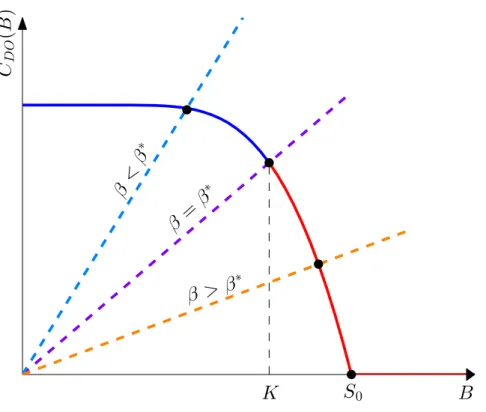
Figure 3.1: The solution of CDO(0, S0;K, T, B) = B/β. Two solid lines in different

colours are the form ofCDO(B) depending on the value of B.

These all together show that there exists a unique root of the transcendental equation (3.2.5) forβ ∈[0,∞]. Write the transcendental equation (3.2.5) as

CDO(0, S0;K, T, B) =

B

β. (3.2.6)

Consider this as an intersection between a curve CDO(0, S0;K, T, B) and a straight

line B/β. Since the unique solution B of the equation (3.2.6) changes with different values ofβ, we define a boundary valueβ∗at which (3.2.6) achieves its unique root at

B =K. Figure 3.1 shows the result. We obtainβ∗ explicitly by substituting B =K

into (3.2.6), which gives

β∗ = K CDO(0, S0;K, T, K) = K CBS(0, S0;K, T)− S0 K 2α CBS 0,K 2 S0 ;K, T . (3.2.7)

Pricing the self-referential down-and-out call option follows in straightforward way. Ifβ < β∗ forβ∗ given as (3.2.7), then solve a transcendental equation

B β =CBS(0, S0;K, T)− S0 B 2α CBS 0,B 2 S0 ;K, T .

(23)

Ifβ > β∗, then solve B β =CBS(0, S0;B, T) + (B−K)Cd(0, S0;B, T) − S0 B 2α CBS 0,B 2 S0 ;B, T + (B−K)Cd 0,B 2 S0 ;B, T .

Since the transcendental equation depends on S0,K, T, andβ, write the root of the

equation as

B = ˜B(S0, K, T, β).

Then simply the price of the down-and-out call option is

CDO(t, S;K, T,B˜),

whereCDO(·) is a price function of standard down-and-out call options.

3.2.2 Self-referential down-and-out put options

We start with introducing the price function of a standard down-and-out put option. In order for the put option to be exercised at maturity, we need S < K. Hence if

K < B, the option is worthless since the underlying will always hit the barrierB and knocked-out first before it has positive payoff. Define a function

V(t, S;K, T, B) =PBS(t, S;K, T)−PBS(t, S;B, T)−(K−B)Pd(t, S;B, T),

then the value of down-and-out put option is

PDO(t, S;K, T, B) = V(t, S;K, T, B)− S B 2α V t,B 2 S ;K, T, B ,

for B < K. We define the barrier of a self-referential down-and-out put option similarly,

B =β PDO(0, S0;K, T, B), (3.2.8)

for some constantβ >0.

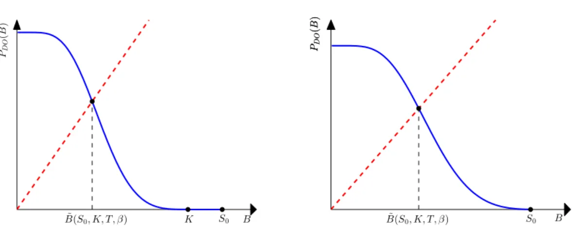
The price function of the down-and-out put option is a decreasing function of the barrier B, starts from PDO(t, S;K, T,0) >0 at B = 0 and stays at zero for B ≥ K.

We consider two cases:

1. If S0 ≥K, the option price is defined fromPDO(0, S0;K, T,0) at B = 0 to 0 at

B ∈ [K, S0]. Thus, there exists a unique root to the transcendental equation

(3.2.8) for all values of β >0.

2. If S0 < K, the option price range is the same but, in this case, the option first

hits zero atS0, notK. So there still exists a unique root to the transcendental

(24)

K S0 ˜ B(S0, K, T,β) PD O ( B ) B B˜(S0, K, T,β) S0 PD O ( B ) PD O ( B ) B

Figure 3.2: The solution ˜B(S0, K, T, β) ofPDO(0, S0;K, T, B) =B/β. The graph on

right-hand side is whenK < S0, whereas the graph on left-hand side is whenK ≥S0.

Pricing the option is exactly the same as down-and-out call option. We assume that the root of (3.2.8) is

B = ˜B(S0, K, T, β).

Then the price of the self-referential down-and-out put option is

PDO(t, S;K, T,B˜).

3.2.3 Stability of the solution of down-and-out options

Note that the down-and-out options decrease in value as the barrier increases. More-over, there exists a unique solution to the transcendental equations for all β > 0. Hence we get the stability condition as before,

β∂VDO ∂B <1.

In order for the solution to be stable, we require

β < β_s∗ = 1 ∂VDO ∂B (0, S0;K, T,B˜) ,

where VDO is a value function of either down-and-out call or put options. If given

β is smaller than β_s∗, then the root of the transcendental equation is stable. First

B-derivatives of the down-and-out barrier option value functions can be found in Appendix B.

Interpretation follows the same with the self-referential forward-start call option. By forcing up the down-and-out option price, we decrease the barrier in the transcen-dental equation, i.e. perturbing the option price results in the barrier to move in the opposite direction. Hence the decrease in the barrier offsets the effect of forcing up the option price and we expect the root of the transcendental equation to be stable under certain condition.

(25)

K

B

˜

S

₀

β

>

β

∗ c

β

=

β

∗c

β

<

β

∗c

C

D I

(

B

)

B

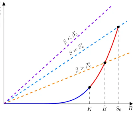
Figure 3.3: The solution ˜B(S0, K, T, β) ofCDI(0, S0;K, T, B) =B/β. Again the two

solid lines in different colours are the form ofCDI(B) depending on the value of B.

3.3 Self-referential down-and-in options

For a down-and-in and a down-and-out options, if they have the same parameters and option type, only one will be available at maturity. This is because if the underlying asset hits the barrier, one will be activated whereas the other will be knocked out. Similarly, if the underlying never hits the barrier, one will never be activated whereas the other survives until the maturity. Hence, we have out-in parity:

Down-and-in + Down-and-out = European.

So we get price functions of down-and-in options according to the out-in parity,

CDI(t, S;K, T, B) = CBS(t, S;K, T)−CDO(t, S;K, T, B),

PDI(t, S;K, T, B) =PBS(t, S;K, T)−PDO(t, S;K, T, B).

We assume that the barrierB is decided at time zero in the same way as (3.2.4).

3.3.1 Self-referential down-and-in call options

We define the barrier of a self referential down-and-in call option as

(26)

K

S

₀

˜

B

˜

B

1

B

˜

2

˜

B

3

β

∗p

<

β

∗∗p

<

β

<

β

∗ p

β

=

β

∗ ∗ p

β

<

β

∗∗_p

P

D I

(

B

)

B

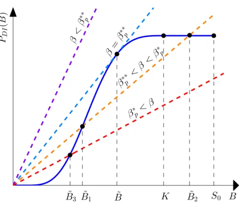
Figure 3.4: The solution ˜B(S0, K, T, β) ofPDI(0, S0;K, T, B) =B/β.

We assumed that the underlying risky asset follows the dynamics of a geometric Brownian motion and the underlying value is non-zero almost surely. Hence, if the barrier is zero, the option will never be activated and the option price is zero. This shows that there exists a trivial solution of (3.3.9) at B = 0.

Existence of non-trivial solutions depend on the value ofβ. Note that the function

CDI(0, S0;K, T, B) is a strictly increasing in B. Since we are only considering the

regionB ≤S0, the smallest possibleβvalue is at which the straight lineB/βintersects

with CDI(0, S0;K, T, B) is at B =S0. Figure 3.3 shows the result clearly. We define

suchβ as β_c∗. Thenβ_c∗ satisfies

β_c∗ = S0

CDI(0, S0;K, T, S0)

.

There exists a non-trivial root of (3.3.9) if β ≥ β_c∗ and the option price follows from exactly same argument as down-and-out case. If β < β_c∗, there only exists a trivial root and the self-referential down-and-in call option does not exist.

3.3.2 Self-referential down-and-in put options

We define the barrier in the same way,

(27)

The same argument with the down-and-in call option shows that the equation also has a trivial solution atB = 0. The fact that a down-and-out put option is worthless for B ≥ K and the out-in parity shows that the down-and-in put option becomes a standard European put for B ≥ K. We verified that the same results hold for two cases,S0 ≥K andS0 < K, in finding the root of the transcendental equation. So we

assumeS0 ≥K in this problem and expect the parallel result for S0 < K.

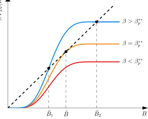
If we look for non-trivial solutions, four cases arise and Figure 3.4 clearly shows the following four cases:

1. If β is too small, there is no non-trivial solution of the equation (3.3.10). 2. If β is equal to the critical valueβ_p∗∗, there exists one non-trivial root.

3. If β is larger than the critical value β_p∗∗ and smaller or equal to another critical valueβ_p∗, there exists two strictly positive roots.

4. If β is larger thanβ_p∗, there exists only one non-trivial root.

It is straightforward to find the second critical valueβ_p∗. By equating the gradient of a straight line which crosses (S0, PDI(0, S0;K, T, S0)) and 1/βp∗, we get

β_p∗ = S0

PDI(0, S0;K, T, S0)

.

This is the corresponding result of the critical value of down-and-in call option.

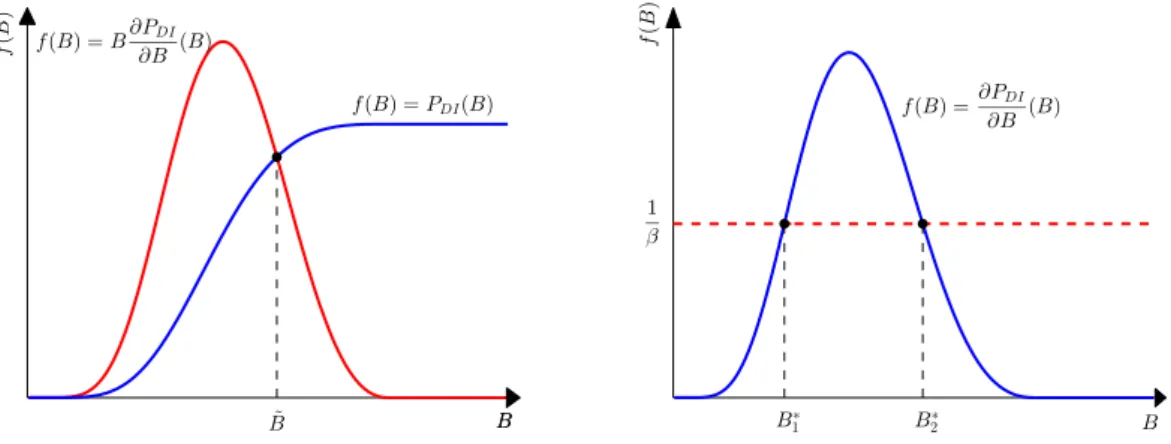
The critical valueβ_p∗∗is determined by the condition that the curvePDI(0, S0;K, T, B)

and the line B/β meet tangentially at β =β_p∗∗ and B = ˜B. That is, β_p∗∗ and ˜B will be defined by the solution of the following nonlinear simultaneous equations

B =β PDI(0, S0;K, T, B),

1 = β∂PDI

∂B (0, S0;K, T, B),

(3.3.11)

wherePDI(0, S0;K, T, B) is defined as above and

∂PDI ∂B = (K−B) σB√T e −rT N0−d(1)₋ + S0 B 2α N0−d(2)₋ ! − S0 B 2α 2B S0 N−d(3)₊ −N−d(2)₊ +2α B V 0,B 2 S0 ;T, K, B , with d(1)± = log(S0/B) + (r± 1₂σ2)T σ√T , d(2)± = log(B/S0) + (r± 1₂σ2)T σ√T , d(3)_± = log(B 2_/S 0K) + (r± 1₂σ2)T σ√T .

(28)

B f(B) =B∂PDI ∂B (B) f(B) =PDI(B) B ˜ B f ( B ) f(B) =∂PDI ∂B (B) B B∗ 1 B∗2 f ( B ) 1 β

Figure 3.5: The graph on the left-hand side shows the existence of the solution of the equation (3.3.12) whereas the graph on the right-hand side shows the possible two candidate solutions of (3.3.12).

Eliminating β gives

B∂PDI

∂B (0, S0;K, T, B) =PDI(0, S0;K, T, B). (3.3.12)

Note thatPDI(0, S0;K, T, B) is a strictly increasing function of B ∈[0, K] and stays

constant forB ∈[K, S0]. Moreover, we have

∂PDI ∂B B=0 = ∂PDI ∂B B=K = 0.

SincePDI(0, S0;K, T, B) is a constant for B ∈[K, S0], we also have

∂PDI ∂B _B∈ [K,S0] = 0.

The function ∂PDI/∂B starts from zero at B = 0 and increases monotonically until

it achieves its maximum. Then the function is monotonic decreasing until it hits zero again at B =K and stays at zero for B ∈ [K, S0]. So there exists a trivial solution

at B = 0. Since the non-trivial solution is of our interest, we consider the order of functions for smallB,

PDI ∼ O e−12(logB) 2 B2α_log_B ! , ∂PDI ∂B ∼ O e−12(logB) 2 B2α+1 ! , B∂PDI ∂B ∼ O e−12(logB) 2 B2α ! .

(29)

Hence, for B close to zero, we get

B∂PDI

∂B (0, S0;K, T, B)> PDI(0, S0;K, T, B).

When two functions start from B = 0, the function B(∂PDI/∂B) lies above PDI.

Since PDI is increasing and B(∂PDI/∂B) will hit zero again atB =K, there always

exists a solution to (3.3.12). The graph on the left-hand side of Figure 3.5 clearly shows this result.

The graph on the right-hand side Fingure 3.5 shows that there exists only two candidates for the solution of the nonlinear simultaneous equations (3.3.11), B₁∗ and

B₂∗ which satisfy β ∂PDI ∂B B=B∗ 1,B2∗ = 1.

We assume that B₁∗ < B₂∗. Considering the order of PDI(B) for small B, it is clear

that

β PDI(B)< B

for B close to zero which means that from B = 0, the straight line f(B) = B lies aboveβ PDI(B). For B ∈[0, B1∗],β(∂PDI/∂B) is an increasing function and

β ∂PDI ∂B _B∈ [0,B˜1) <1. (3.3.13)

Now we assumeB₁∗ is a solution to (3.3.11), i.e.

B₁∗ =β PDI(0, S0;K, T, B1∗),

1 =β∂PDI

∂B (0, S0;K, T, B

∗

1).

Then according to the mean value theorem, there exists B ∈(0, B₁∗) such that 1 =β∂PDI

∂B (0, S0;K, T, B)

and this contradicts (3.3.13). Hence B∗₂ is the only possible solution and this proves the uniqueness of the solution of (3.3.11).

If we define the solution of (3.3.12) as ˜B(S0, K, T) then the critical value βp∗∗ is

simply β_p∗∗ = ˜ B PDI(0, S0;K, T,B˜) .

Pricing of the option follows exactly the same as before. Compare given β with the critical values to decide how many non-trivial roots the transcendental equation (3.3.10) has. Then solve numerically to obtain the roots of (3.3.10) and substitute intoP(t, S;K, T, B) to get the price of the option at time t.

(30)

3.3.3 Stability of the solution of down-and-in options

Since neither of the existence nor uniqueness of the root of the transcendental equation is guaranteed, we need to consider more cases than simply applying the stability condition (2.2.8). Since it is clear that all the trivial roots of the transcendental equations are stable, we will only consider non-trivial roots in this section.

For down-and-in call options, there exists a non-trivial root to the transcendental equation (3.3.9) ifβ ≥β_c∗. The stability condition of the root B = ˜B is

β ∂CDI ∂B (0, S0;K, T, ˜ B) <1. So we also require β < 1 ∂CDI ∂B (0, S0;K, T, ˜ B) . (3.3.14) Note that ∂CDI ∂B B=0 = 0,

and this clearly shows that for the trivial root B = 0 β ≥β_c∗, the condition (3.3.14) is satisfied for allβ. Now we check the existence of β satisfying

β_c∗ ≤β < 1 ∂CDI ∂B (0, S0;K, T, ˜ B) .

for a non-trivial root B = ˜B. First, consider functions CDI(0, S0;K, T, B) and the

first B-derivative of CDI(0, S0;K, T, B) in Appendix B and note that they are both

increasing functions of B. For B close to zero, CDI(0, S0;K, T, B) has the leading

order CDI ∼ O e−2(logB)2 B2α_log_B ! .

Hence the curve of the functionβ CDI(B) lies below a straight linef(B) =B when it

starts from B = 0. Since the first B-derivative is an increasing function of B, when the curve first meet the straight line, the gradient of the curve is always greater than the gradient of the straight line, i.e.

∂CDI ∂B B= ˜B >1,

and this shows that the stability condition will never be met. So there is noβ value at which the stability of the root is guaranteed for down-and-in call option.

For down-and-in put options, we consider stability of roots for each of four different cases of β values.

(31)

˜

B

˜

B

₁

B

˜

₂

β

>

β

∗∗ p

β

=

β

∗∗ p

β

<

β

∗∗ p

β

P

D I

(

B

)

B

Figure 3.6: The figure shows graphs of β PDI(0, S0;K, T, B) as a function of B for

different values ofβ. The dashed black line is a straight line with gradient one. Hence, by comparing the gradient ofβ PDI(B) at ˜B1 and ˜B2 with the gradient of the straight

line, we expect ˜B2 to be a stable solution whereas ˜B1 is guaranteed to be stable.

2. If β =β_p∗∗, from the nonlinear simultaneous equations (3.3.11), we have

1 =β_p∗∗∂PDI

∂B (0, S0;K, T, B),

and the stability condition is not satisfied,

f0(B) = β_p∗∗∂PDI

∂B (0, S0;K, T, B)≮1.

Hence the non-trivial is not guaranteed to be stable.

3. If β_p∗∗ < β < β_p∗, define two non-trivial roots as ˜B1 and ˜B2. Then we have

0<B˜1 <B <˜ B˜2 < S0 where ˜B is a non-trivial root of the case β =βp∗∗. The

same argument used to show the uniqueness of the solution of the nonlinear simultaneous equations shows that

β ∂PDI ∂B B= ˜B1 >1.

(32)

The stability condition needs to be checked to determine whether ˜B2 is stable

or not. So we get a stable solution ˜B2 if

β < 1 ∂PDI ∂B (0, S0;K, T,B˜2) .

4. If β > β_p∗, similar toB = ˜B1, the stability of the solution is not guaranteed.

The same interpretation with the self-referential forward-start put option applies. Perturbing the option price in the transcendental equation leads the barrier to move in the same direction with the perturbation and this will increase the option price again. Hence the root of the equation will blow up and we expect the root to be unstable.

(33)

Chapter 4 Self-referential Asian options

This chapter closely follows the chapter ofNonlinear Asian optionsof [2] and the last section ofThe zero volatility case without the similarity reduction is a new extension of the reference. An Asian option is an option whose payoff depends on the average of the underlying asset price over the life, or some part of the life, of the option. If we assume that arithmetic averages are taken over the life of the option, the payoff depends on 1 T T Z 0 Stdt.

Define a stochastic process Jt such that

Jt= t

Z

0

Sτdτ.

By assuming the Markov property and the standard hedging argument with Itˆo’s lemma shows that the the Asian option priceV(·) satisfies

∂V ∂t + 1 2σ 2_S2∂2V ∂S2 + (r−q)S ∂V ∂S +S ∂V ∂J −rV = 0, V(T, S, J) = Ψ(S, J/T),

where Ψ(·) is the payoff function, and the partial differential equation holds forS >0,

J >0 and 0≤t < T.

Now we consider a self-referential Asian option where the option payoff depends on the arithmetic average of the option value itself. So the payoff now depends on the term 1 T T Z 0 Vtdt.

(34)

mod-ifying the process Jt as Jt = t Z 0 Vτdτ.

The process Jt now follows the dynamics

dJt=Vtdt.

Then applying the same argument shows that the option price satisfies

∂V ∂t + 1 2σ 2_S2∂2V ∂S2 + (r−q)S ∂V ∂S +V ∂V ∂J −rV = 0, V(T, S, J) = Ψ(S, J/T). (4.0.1)

The partial differential equation again holds for S >0 and 0≤t < T, but the range ofJ values is not necessarily the same. If we have a negative payoff, the option price can become negative, and there is no guarantee that the arithmetic average of the option value is positive.

4.1 Linear payoffs

We consider a self-referential Asian option whose payoff is linear. If we assume the payoff function is

Ψ(S, J/T) = AS+BJ +C,

whereA,B, andC are constants, then we expect the price function of the form

V(t, S, J) = a(t)S+b(t)J+c(t).

By substituting this into (4.0.1) and setting the independent term and coefficients of

S and J equal zero, we get a system of ordinary differential equations with terminal conditions: ˙ a=a(q−b), a(T) =A, ˙ b =b(r−b), b(T) =B, ˙ c=c(r−b), c(T) = C.

By solving this, we get

a(t) = rAe −q(T−t) r−B(1−e−r(T−t)₎, b(t) = rBe −r(T−t) r−B(1−e−r(T−t)₎, c(t) = rCe −r(T−t) r−B(1−e−r(T−t)₎.

(35)

Note that these solutions blow up if

r=B(1−e−r(T−t)).

Forr >0 and r≥B,

r≥B > B(1−e−r(T−t)), (4.1.2) and, hence, the solutions stay finite. But if B > r, there exists t∗ < T where the solutions become infinite,

t∗ =T + 1 rlog 1− r B < T. (4.1.3)

4.2 Average-strike call and put options

We define an average-strike call option as an option with payoff max S− J T,0 ,

and the payoff of an average-strike put option as max J T −S,0 .

In order to compute the price functions of such options, we approach with solving the Black-Scholes PDE (4.0.1). First, note that both of these payoffs satisfy

Ψ S,J T =SΨ 1, J T S .

Then we simplify the problem by introducing dimensionless variables,

τ = 1− t T, ξ = J T S, φ= V S. If we write V(t, S, J) = S φ(τ, ξ),

then, by the chain rule, we get

∂V ∂t =− S T ∂φ ∂τ, ∂V ∂S =φ−ξ ∂φ ∂ξ, ∂2_V ∂S2 = ξ2 S ∂2_φ ∂ξ2, ∂V ∂J = 1 T ∂φ ∂ξ

and the partial differential equation (4.0.1) becomes

∂φ ∂τ =α 2_ξ2∂ 2_φ ∂ξ2 + (φ−βξ) ∂φ ∂ξ −γφ, φ(0, ξ) = Ψ(1, ξ) = f(ξ), (4.2.4) where α2 = 1 2σ 2_{T, β} _{= (}_r₋_q₎_{T, γ} ₌_qT.

Due to the substitution ofτ, the PDE (4.2.4) is forward in time and this is an initial value problem with given initial condition.

(36)

4.3 The zero volatility case

If we assume the volatility σ to be zero, the constant α is zero and (4.2.4) becomes the first-order, quasi-linear problem

∂φ ∂τ + (βξ−φ) ∂φ ∂ξ =−γφ, φ(0, ξ) =f(ξ). (4.3.5)

We achieve the solutions of the initial value problem (4.3.5) by method of character-istics. The characteristic curves of the problem are the integral curves of of the vector field (1, βξ −φ). We look for a specific curve which satisfies the initial parametric condition. Hence we get characteristic equations

∂τ ∂p = 1, τ(0, q) = 0, ∂ξ ∂p = βξ−φ, ξ(0, q) =q, ∂φ ∂p = −γφ, φ(0, q) =f(q).

We solve these to find the parametric solutions,

τ(p, q) =p,

ξ(p, q) =qeβp−e

βp₋_e−γp

β+γ f(q), φ(p, q) =e−γpf(q).

In order to find the solution, we invert the mapping (p, q) → (τ, ξ) and substitute into φ(p, q) to get φ in terms of τ and ξ. If the determinant of the Jacobian matrix is non-zero, we can invert the transformation and get expression of (p, q) in terms of (τ, ξ), det   ∂τ /∂p ∂ξ/∂p ∂τ /∂q ∂ξ/∂q  = ∂ξ ∂q =e βp 1− 1−e −(β+γ)p β+γ f 0 (q) .

If we assume that β+γ =rT >0, then for p≥0 and for all q, the condition of the determinant to be non-zero is equivalent to f0(q) < β+γ. That is, if f0(q)≥ β+γ

for some q, then there always exists p such that the determinant is zero. Note that under the condition of f(·), we have

eβp 1− 1−e −(β+γ)p β+γ f 0 (q) >0.

Thus we get the condition of function f(·) for non-zero determinant independent of

pand q:

(37)

To get the condition in terms of the original variables, write

q = J

T S,

and then the condition follows by

f0(q) = Ψ0(1, q) = ∂J ∂ J T S ∂ ∂JΨ 1, J T S =T S ∂ ∂JΨ 1, J T S =T ∂ ∂JV(T, S, J)< β+γ =rT.

Therefore, we get the condition in the original variables

∂

∂JV(T, S, J)< r. (4.3.7)

If the Jacobian determinant vanishes, the transformation is not invertible. In this case, there is a singularity in the solution of the original problem (4.3.5). This occurs when

1−e−(β+γ)p

β+γ f

0

(q) = 1. (4.3.8)

For p ≥ 0 and β+γ > 0, the condition is only satisfied when f0(q) > β +γ. Note that τ = p and the time when the singularity first develops could be achieved by finding the minimum p which satisfies (4.3.8). We call this pair of (p, q) as (p∗, q∗). The minimump takes place at the maximumf0(q). So we get

q∗ = arg max q f0(q), p∗ =− 1 β+γ log 1− β+γ f0₍_q∗₎ . (4.3.9)

In terms of the original variables, the singularity first develops at (τ∗, ξ∗) where

τ∗ =p∗, ξ∗ =q∗eβp∗− e

βp∗₋_e−γp∗

β+γ f(q

∗

). (4.3.10)

4.3.1 The average-strike call options

The payoff of the self-referential average-strike call option is

Smax 1− J T S,0 =Smax{1−ξ,0}.

This provides the initial condition of the problem (4.3.5) as

(38)

Note that we have f0(ξ) = −1{ξ<1} ≤ 0 and the function f(·) satisfies the condition

(4.3.6). Hence, we can invert the transformation and get

p=τ, q =          (β+γ)ξ+eβτ −e−γτ (β+γ)eβτ ₊_eβτ ₋_e−γτ for ξ < e βτ_, ξ e−βτ for ξ ≥eβτ.

Then by substituting this intoφc(p, q), we get

φc(τ, ξ) =          (β+γ)e−γτ(1−ξ e−βτ) β+γ+ 1−e−(β+γ)τ for ξ < e βτ_, 0 for ξ ≥eβτ. (4.3.11)

There is no singularity in this solution since we assumeβ+γ >0 and then

β+γ+ 1−e−(β+γ)τ > β+γ >0,

for all τ ≥0.

4.3.2 The average-strike put options

For the self-referential average-strike put option, we find the initial condition from the payoff,

φp(0, ξ) = g(ξ) = max{ξ−1,0}.

In this case,g0(ξ) = 1{ξ>1} and if β+γ <1, then there exists a pair (τ∗, ξ∗) at which

the singularity arises in the solution. We find such pair by (4.3.9) and (4.3.10). First, compute (p∗, q∗) by (4.3.9): q∗ = arg max q g0(q) = (1,∞), p∗ =− 1 β+γ log (1−β−γ). (4.3.12)

This shows that we get singularity for a range of values ofξ. If we proceed the same as call case, inverting the transformation gives

p=τ, q =          ξ e−βτ for ξ ≤eβτ_, (β+γ)ξ−eβτ ₊_e−γτ (β+γ)eβτ ₋_eβτ ₊_e−γτ for ξ > e βτ_,

and by substitution, we get

φp(τ, ξ) =          0 for ξ≤eβτ_, (β+γ)e−γτ(ξ e−βτ −1) β+γ−1 +e−(β+γ)τ for ξ > e βτ_. (4.3.13)

(39)

The solution has a singularity atτ =τ∗ where τ∗ satisfies 1−β−γ =e−(β+γ)τ∗,

and it occurs along the entire intervalξ > eβτ∗_{. Rearrange this and get} _τ∗ _explicitly:

τ∗ =− 1

β+γ log(1−β−γ),

and this result indeed agrees with (4.3.12), since we have τ =p.

The option price with singularities is an inappropriate result and financial in-terpretation is not very clear. So we try to include the diffusion term (the second

ξ-derivative term) in the problem and expect to achieve more sensible results.

4.4 The small volatility limit

In this section, we analyse the effect of the diffusion term in the partial differential equation by including it in a small region around ξ =eβτ_{. There are discontinuities}

of the option value in the first ξ-derivative along the curve ξ = eβτ_{. So we expect}

smoothing out effect by including the diffusion term in the small region. Hence for

δ1, consider two regions:

i) The outer region where ξ−eβτ δ.

ii) The inner region whereξ−eβτ ₌_O₍_δ_{). In this region, we introduce a new scaled}

variable ζ = ξ−e βτ δ , ξ =e βτ +δζ.

Then the scaling ofφ(·) follows from the initial conditions of put and call options,

ψ(τ0, ζ) =α φ(τ, ξ).

We now get the partial differential equation (4.2.4) in terms of the new variables by the transformation (τ, ξ)→(τ0, ζ). By the chain rule,

∂ ∂τ = ∂ ∂τ0 − β δe βτ ∂ ∂ζ, ∂ ∂ξ = 1 δ ∂ ∂ζ, ∂2 ∂ξ2 = 1 δ2 ∂2 ∂ζ2

and using this gives

δ∂ψ ∂τ0 = α2 δ (e βτ0 ₊_δζ₎2∂2ψ ∂ζ2 +δ(ψ−β ζ) ∂ψ ∂ζ −γ δ ψ.

We choose δ=α, i.e. σ2 _r_{, and substitute the specified} _δ_:

∂ψ ∂τ0 = (e βτ0 ₊_αζ₎2∂ 2_ψ ∂ζ2 + (ψ−β ζ) ∂ψ ∂ζ −γ ψ.

(40)

For small α, the partial differential equation of the inner problem becomes simpler by excluding the term with α

∂ψ ∂τ0 =e 2βτ0∂2ψ ∂ζ2 + (ψ−β ζ) ∂ψ ∂ζ −γ ψ.

Since we set δ = α, the solution for the zero volatility case in the previous section should match with the outer region solution. Thus, we get boundary conditions of the problem for put and call options from (4.3.11) and (4.3.13):

1. For the average-strike call options,

ψc(0, ζ) = max(0,−ζ), lim ζ→−∞ψc(τ 0 , ζ) =− (β+γ)e−(β+γ)τ β+γ+ 1−e−(β+γ)τ ζ, lim ζ→∞ψc(τ 0 , ζ) = 0.

2. For the average-strike put options,

ψp(0, ζ) = max(0,−ζ), lim ζ→−∞ψp(τ 0 , ζ) = 0, lim ζ→∞ψp(τ 0 , ζ) = − (β+γ)e−(β+γ)τ β+γ+ 1−e−(β+γ)τ ζ.

Because the conditions at ζ → ±∞ (−∞ for call and +∞ for put) blow up at the same time as the zero volatility problem, we conjecture that the solution of the inner problem blows up at the same time. That is, volatility, or the diffusion term, is not effective in preventing singularities in the solutions. The full problem with σ not small and σ >0 must be solved numerically.

4.5 The zero volatility case without the similarity

reduction

The similarity reduction inThe zero volatility case section does not apply to all pay-offs. For example, the method does not apply for average-rate options, i.e. options with payoff max{J/T−K,0}or max{K−J/T,0}. In this section, under the assump-tion of zero volatility again, we derive price funcassump-tions and condiassump-tions on the payoff of the self-referential Asian options at which singularities in the option prices occur by solving the partial differential equation (4.0.1) directly. For zero volatility, the original partial differential equation is

∂V ∂t + (r−q)S ∂V ∂S +V ∂V ∂J −rV = 0, V(T, S, J) = Ψ(S, J/T).

(41)

We attempt to solve this by the method of characteristics again. Introducing a new time variable

t0 =T −t (4.5.14)

to get the forward in time partial differential equation

∂V ∂t0 −(r−q)S ∂V ∂S −V ∂V ∂J =−rV, V(T, S, J) = Ψ(S, J/T).

Then we get characteristic equations

∂t0 ∂τ = 1, τ(0) = 0, ∂S ∂τ = −(r−q)S, S(0) =s, ∂J ∂τ = −V, J(0) =j, ∂V ∂τ = −rV, V(0) = Ψ(s, j/T).

By solving this, we get

t0 = τ, S = s e−(r−q)τ, J = j −1 r 1−e −rτ Ψ(s, j/T), V = Ψ(s, j/T)e−rτ.

We invert to write (τ, s, j) in terms of (t0, S, J) and substitute into V(τ, s, j) to get the price function. Hence we consider the determinant of the Jacobian matrix again

det      ∂t0/∂τ ∂t0/∂s ∂t0/∂j ∂S/∂τ ∂S/∂s ∂S/∂j ∂J/∂τ ∂J/∂s ∂J/∂j      =e−(r−q)τ 1−1 r 1−e −rτ ∂ ∂jΨ(s, j/T) .

The transformation is only invertible if the determinant is non-zero. The same argu-ment as before shows that the determinant is always non-zero if

∂

∂jΨ(s, j/T)< r

for all positive s and j. Since the condition is on the function, not variables, we get the condition on the payoff by replacing s toS and j to J:

∂

(42)

This clearly agrees with (4.3.7) since this is the same but more generalised problem. Some payoffs seem to give blow-up especially if the payoff is increasing in J. We expect the reason from the condition on the payoff (4.5.15). If the condition is not satisfied, i.e.

∂

∂JV(T, S, J)> r,

there exists some times at which the transformation is not invertible and this is when the solution blows-up. Consider the case of the linear payoff as an example. In (4.1.2) and (4.1.3), we showed that the solution explodes at some time for B > r. The non-zero Jacobian determinant condition (4.5.15) for the linear payoff is

∂

∂JV(T, S, J) = ∂

∂J(AS+BJ +C) = B < r. (4.5.16)

The time at which the condition (4.5.16) is not satisfied exactly overlaps with the condition onB we derived in the linear payoff section.

4.5.1 The average-rate call options

The payoff of the average-rate call option is

max

J

T −K,0

for some constantK. The firstJ-derivative of the payoff is

∂ ∂J max J T −K,0 = 1 T 1{J >KT}

and the condition (4.5.15) is not satisfied if J > KT and rT < 1. So we expect singularities in the price function at some times.

Now we invert the mapping (t0, S, J)→(τ, s, j) to price the option. The inverted mapping is τ = t0, s = S e(r−q)t0, j =          J for J ≤KT, rT J −KT(1−e−rt0) rT −(1−e−rt0 ) for J > KT.

Then substituting into V(τ, s, j) gives the option price in terms of the original vari-ables: V(τ, s, j) = Ψ(s, j/T)e−rτ =          0 for J ≤KT, r(J −KT)e−rt0 rT −(1−e−rt0 ) for J > KT.

(43)

wheret0is defined as (4.5.14). As we discussed with the non-zero condition of Jacobian determinant, the option price indeed blows up at some time ifrT <1. More precisely, the option price blows up at

t0 = 1 r log 1 1−rT .

4.5.2 The average-rate put options

We proceed with the same argument as the average-rate call options but with different payoff max K− J T,0

for some constant K. We check the condition (4.5.15) by differentiating the payoff with respect toJ: ∂ ∂J max K− J T,0 =−1 T 1{J <KT} ≤0.

So forr >0, the condition is satisfied and the mapping is always invertible. Then we invert the mapping (t0, S, J)→(τ, s, j) and get

τ = t0, s = S e(r−q)t0, j =          rT J +KT(1−e−rt0) rT + (1−e−rt0 ) for J ≤KT, J for J > KT.

We similarly obtain the option price by substituting into V(τ, s, j):

V(τ, s, j) = Ψ(s, j/T)e−rτ =          r(KT −J)e−rt0 rT + (1−e−rt0 ) for J ≤KT, 0 for J > KT.

(44)

Chapter 5 Conclusion

In this thesis, we investigated three different types of exotic options with self-referential property. We mainly focused on pricing the options and analysing and interpreting the features of the option prices. Initially, the carbon market model is introduced as motivation of the thesis. Then we moved on to the self-referential forward-start options and derived the prices and the stability conditions of the self-referential op-tions. We also showed that the price of the self-referential call option is well-defined whereas the the self-referential put option does not exist under certain conditions on its parameters. When the put price does exist it is mathematically and financially un-stable. We applied the same idea to barrier options and found that the self-referential down-and-out option prices are well-defined, unlike to the down-and-in option prices. The problem of both forward-start and barrier options essentially reduces down to solve transcendental equations. We only analysed the existence and stability of the roots but the roots can be computed numerically by the Newton’s iteration or the bisection method in a straightforward way. Finally, we introduced and formulated the problem of the self-referential Asian options. Since Asian options are path-dependent, the problem does not develop to simply solve a transcendental equation. We chose to approach the problem with the partial differential equation method. Due to the nonlinearity of the PDE, we made assumptions of the zero volatility and the small volatility. In both cases, we observed that the option price blows up at some time if the payoff does not satisfy certain condition. The singularities in the option price is inappropriate and cannot be interpreted financially. Therefore, we conclude by conjecturing that this is due to the assumption on the volatility.

Further research on referential options may include the extension of the self-referential Asian options. One may numerically solve the full nonlinear PDE without any assumptions to examine the singularities in the option price. Self-referential versions of lookback or American options may also be considered as new areas of research.

(45)

(46)

Appendix A

Barrier option price functions

The following functions are taken from [7]. We assume the dividend rateq is zero.

A.0.3 Down-and-out call option

CDO =CBS(S,max{B, K})− S B 2α CBS B2 S ,max{B, K} + (max{B, K} −K)e−r(T−t) × N(d−(S,max{B, K}))− S B 2α N d− B2 S ,max{B, K}

A.0.4 Down-and-out put option

PDO = PBS(S, K)−P(S, B) + (B−K)e−r(T−t)N(−d−(B, S)) 1{K>B} − S B 2α PBS B2 S , K −PBS B2 S , B + (B−K)e−r(T−t)N(−d−(B, S)) 1{K>B}

A.0.5 Down-and-in call option

CDI = PBS(S, K)−PBS(S, B) + (B −K)e−r(T−t)N(−d−(S, B)) 1B>K + S B 2α CBS B2 S ,max{B, K} +(max{B, K} −K)e−r(T−t)N d− B2 S ,max{B, K}

A.0.6 Down-and-in put option

PDI = S B 2α CBS B2 S , K −CBS B2 S , B −(B−K)e−r(T−t)N(d−(B, S)) 1{K>B} +

PBS(S,min{B, K})−(min{B, K} −K)e−r(T−t)N(−d−(S,min{B, K}))

(47)

A.0.7 Up-and-out call option

CU O = CBS(S, K)−C(S, B)−(B−K)e−r(T−t)N(d−(S, B)) 1{B>K} − S B 2α CBS B2 S , K −CBS B2 S , B −(B−K)e−r(T−t)N(d−(B, S)) 1{B>K}

A.0.8 Up-and-out put option

PU O =PBS(S,min{B, K})− S B 2α PBS B2 S ,min{B, K} −(min{B, K} −K)e−r(T−t) × N(−d−(S,min{B, K}))− S B 2α N −d− B2 S ,min{B, K}

A.0.9 Up-and-in call option

CU I = S B 2α PBS B2 S , K −PBS B2 S , B + (B −K)e−r(T−t)N(−d−(B, S)) 1{B>K}

+CBS(S,max{B, K}) + (max{B, K} −K)e−r(T−t)N(d−(S,max{B, K}))

A.0.10 Up-and-in put option

PU I = CBS(S, K)−CBS(S, B)−(B−K)e−r(T−t)N(d−(S, B)) 1K>B + S B 2α PBS B2 S ,min{B, K} −(min{B, K} −K)e−r(T−t)N −d− B2 S ,min{B, K}

(48)

Appendix B

First

B

-derivative of down-and-in

and down-and-out option price

functions

We assume q= 0 again.

B.0.11 Down-and-out call option

∂CDO

∂B =− ∂CDI

∂B

B.0.12 Down-and-out put option

∂PDO

∂B =− ∂PDI

∂B

B.0.13 Down-and-in call option

∂CDI ∂B =                                    2 S B 2α (1−α) B S Nd(1)₊ +α K B e−r(T−t)Nd(1)− for 0≤B < K, S σ B√T −t 1− K B N0d(2)− + S B 2α (B −K) σ S√T −tN 0_d(3) + for K ≤B, +2 S B 2α (1−α) B S Nd(3)₊ +α K B e−r(T−t)Nd(3)−

(49)

where d(1)_± = log(B 2_{/S K}_{) + (}_r_± 1 2σ 2₎₍_T ₋_t₎ σ√T −t , d(2)_± = log(S/B) + (r± 1 2σ 2₎₍_T ₋_t₎ σ√T −t , d(3)_± = log(B/S) + (r± 1 2σ 2₎₍_T ₋_t₎ σ√T −t .

B.0.14 Down-and-in put option

∂PDI ∂B = (K−B) σB√T −te −r(T−t) _N0₋ d(3)− + S B 2α N0−d(1)− ! − S B 2α 2B S N−d(2)₊ −N−d(1)₊ + 2α B V t,B 2 S ;T, K, B , where V(t, S;K, T, B) = PBS(t, S;K, T)−PBS(t, S;B, T)−(K−B)Pd(t, S;B, T)

(50)

Bibliography

[1] M. Baxter and A. Rennie, Financial calculus: An introduction to derivative pric-ing, Cambridge University Press, 1996.

[2] J.N. Dewynne and S.D. Howison, Nonlinear Options, preprint, 2011.

[3] S. Howison, J. Dewynne and D. Schwarz, Self-referential options, from toy ex-amples to carbon markets, 2010. (Slides of presentation, available at

https://people.maths.ox.ac.uk/howison/OMIJun2010.pdf)

[4] S.D. Howison and D. Schwarz, Risk-neutral pricing of financial instruments in emission markets: A structural approach, SIAM J. Financial Math. 3, 709-739, 2012.

[5] A.G.Z. Kemna and A.C.F. Vorst, A pricing method for options based on average asset values, Journal of Banking & Finance 14, 113-129, 1990.

[6] P. Wilmott, J. Dewynne, and S. Howison, Option pricing, mathematical models and computation, Oxford Financial Press, 1994.

[7] P.G. Zhang,Exotic options, a guide to second generation options, World Scientific Publishing Co. Pte. Ltd, 1998.

Self-Referential Options