Visualisation of structured data through generative probabilistic modeling

(1)

Visualisation of Structured Data through Generative

Probabilistic Modeling

by

Nikolaos Gianniotis

A thesis submitted to The University of Birmingham

for the degree of

DOCTOR OF PHILOSOPHY

School of Computer Science The University of Birmingham September 2007

(2)

University of Birmingham Research Archive

e-theses repository

This unpublished thesis/dissertation is copyright of the author and/or third parties.

The intellectual property rights of the author or third parties in respect of this work

are as defined by The Copyright Designs and Patents Act 1988 or as modified by

any successor legislation.

Any use made of information contained in this thesis/dissertation must be in

accordance with that legislation and must be properly acknowledged. Further

distribution or reproduction in any format is prohibited without the permission of

the copyright holder.

(3)

Abstract

This thesis is concerned with the construction of topographic maps of structured data. A probabilistic generative model-based approach is taken, inspired by the GTM algorithm. De-pending on the data at hand, the form of a probabilistic generative model is speciﬁed that is appropriate for modelling the probability density of the data. A mixture of such models is formulated which is topographically constrained on a low-dimensional latent space. By con-strained, we mean that each point in the latent space determines the parameters of one model via a smooth non-linear mapping; by topographic, we mean that neighbouring latent points gen-erate similar parameters which address statistically similar models. The constrained mixture is trained to model the density of the structured data. A map is constructed by projecting each data item to a location on the latent space where the local latent points are associated with models that express a high probability of having generated the particular data item.

We present three formulations for constructing topographic maps of structured data. Two of them are concerned with tree-structured data and employ hidden Markov trees and Markov trees as probabilistic generative models. The third approach is concerned with astronomical light curves from eclipsing binary stars and employs a physical-based model. The formulation of the all three models is accompanied by experiments and analysis of the resulting topographic maps.

(4)

(5)

Acknowledgements

I would like to express my great appreciation to my supervisor Dr. Peter Tiˇno not only for steering my PhD to interesting directions with thoughtful guidance, but also for inspiring me with excitement to pursue further research in the domain of machine learning in the future.

I would also like to thank Steven Spreckley, Dr. Somak Raychaudhury and Dr. Ian Stevens from the School of Physics and Astronomy, University of Birmingham, for their collaboration and provision of the astronomical model, dataset of light curves and prior distributions in the work presented in chapter 6.

Finally, I could not have completed my PhD studies without the studentship granted by the School of Computer Science, for which I am grateful.

(6)

List of Figures

1.1 Constrained spherical Gaussians. . . 4

2.1 Activation for label of a tree-pattern in SOMSD. . . 14

3.1 Example of an underlying hidden state (states in gray) process emitting labels. . 38

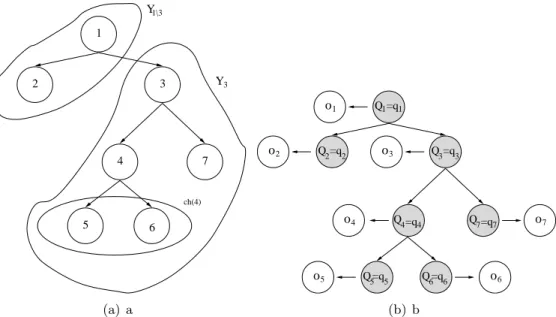
3.2 Notation in tree structures and underlying hidden states. . . 46

3.3 An example of a 3-regular tree. . . 52

3.4 Noisy, intrinsically one-dimensional dataset. . . 55

3.5 Fitted dataset. The means of the mixture of Gaussians belong to a noisy one-dimensional line. . . 59

3.6 Noisy, non-linear, intrinsically one-dimensional dataset. . . 59

3.7 Regularly spaced pointsxc on lineℓ . . . 60

3.8 Fitted dataset: The means of the mixture of Gaussians belong to the one-dimensional lineℓ in Fig. 3.7. . . 61

4.1 Mapping from latent points to the means of Gaussian densities in the data space. 63 4.2 Mapping Γ from latent space_V to the two-dimensional manifold _Mof HMTMs. 68 4.3 Plot of labels for toy and TPB dataset. . . 73

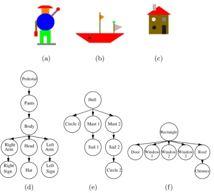
4.4 Example of an image represented as a quadtree. . . 75

4.5 Sample images from TPB. . . 76

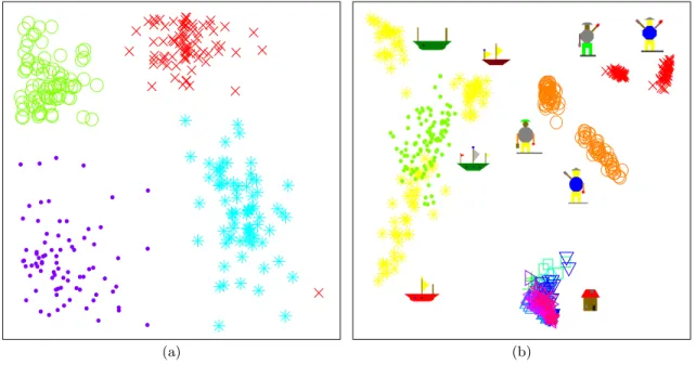
4.6 Visualisation of toy (a) and TPB (b) dataset using GTM-HMTM. . . 77

4.7 TPB task: grid of 2×2-state transition matrices corresponding to the local HMTMs underlying the visualisation plot. . . 79

4.8 TPB task: means of emissions for states k = 1,2 corresponding to the local HMTMs. . . 80

4.9 Visualisation of reduced resolution quadtree dataset (16_×16) for GTM-HMTM. 82 4.10 Quadtree task: grid of 3_×3-state transition matrices corresponding to the local HMTMs underlying the visualisation plot. . . 83

4.11 Quadtree task: means of emissions of GTM-HMTM. . . 83

4.12 Visualisation of toy (a) and TPB (b) dataset using SOMSD. . . 84

4.13 Visualisation of reduced resolution quadtree dataset (8×8) for SOMSD. . . 84

4.14 Evolution of log-likelihood for GTM-HMTM on training and validation set. . . . 87

4.15 Visualisation of toy dataset for GTM-MTM. . . 91

4.16 Visualisation of quadtree dataset (64×64) for GTM-MTM. . . 92

4.17 Evolution of log-likelihood for GTM-MTM on training and validation set. . . 93

5.1 Graph off(x) =₋x2_{. . . .} ₉₅

(10)

5.3 An area element in the latent space subject to magniﬁcation. . . 96

5.4 Two overlapping local patches on a manifold. . . 106

5.5 Two-dimensional manifold_Mof local noise modelsp(_·|x) embedded in manifold Hof all noise models of the same form. . . 108

5.6 Visualisation of toy dataset of binary sequences and Bach chorals. . . 124

5.7 Magniﬁcation factors via FIM (a) and KLD (b) for GTM-HMM on toy dataset. . 125

5.8 Magniﬁcation factors via FIM (a) and KLD (b) for GTM-HMM on Bach chorals dataset. . . 126

5.9 Magniﬁcation factors via FIM (a) and KLD approximation (b) for GTM-HMTM on toy dataset. . . 126

5.10 Magniﬁcation factors via FIM (a) and KLD approximation (b) for GTM-HMTM on TPB dataset. . . 127

5.11 KLD approximation for GTM-HMTM on quadtree dataset. . . 128

5.12 Magniﬁcation factors for GTM-MTM on toy dataset (a). State transitions for 3-rd child node for toy dataset (b). . . 129

6.1 Angles orientating the orbital plane with respect to the plane of sky. . . 134

6.2 Positions of stars and corresponding light curve phases. . . 135

6.3 Phase-shifting and resampling of light curves. . . 137

6.4 Formulation of the topographic mapping model. . . 140

6.5 Linear interpolation on raw light curves. . . 143

6.6 Visualisation of toy dataset. . . 146

6.7 Toy dataset: Heat maps of model parameters. . . 147

6.8 Toy dataset: Topographic map of underlying noise models. . . 148

6.9 Visualisation of real dataset. . . 149

6.10 Real dataset: Heat maps of model parameters. . . 150

6.11 Magniﬁcation factors for GTM-ﬂux on toy dataset. . . 153

6.12 Magniﬁcation factors for GTM-ﬂux on real dataset. . . 154

6.13 SOM for light curves: codebooks may form invalid light curves. . . 156

6.14 A one-dimensional latent space embedded in a higher-dimensional latent space. . 156

E.1 Prior densities on parameters of physical model. . . 182

F.1 Partial eclipse. . . 184

(11)

List of Tables

4.1 Parameters of HMTMs for creating the toy dataset. . . 73

4.2 Classes in TPB dataset. . . 74

6.1 Summary of the areas of the visible discs of the stars. . . 135

(12)

Notation and Abbreviations

A list of the most repeated notation and symbols used in the thesis follows.

Γ Non-linear RBF mapping from spaceV to data/model space

δ(.) Dirac impulse function

δi,j Kronecker delta

D Dataset

DKL[.||.] Kullback-Leibler divergence

Ex[.] Expectation operator with respect to distribution of variable x

θ Parameter vector of probabilistic model

Θ Parameter vector of mixture model

H Space of all models p(_·|x)

L Model likelihood

M Two-dimensional manifold of noise models p(·|x) constrained on latent spaceV N Gaussian distribution

O Light curve from an eclipsing binary system

p(·|x) Local noise model addressed by latent pointx s Sequence data item

t Vector data item

V Latent space embedded in space H

x Coordinate vector of neuron on lattice (in neural-based formulations); Latent point (in GTM formulations)

y Tree data item

W Weight matrix

Wi i-th row of weight matrix

Z Set of indicator-hidden variables EM Expectation-maximisation (algorithm) FIM Fisher information matrix

GTM Generative topographic map (algorithm) HMM Hidden Markov model

HMTM Hidden Markov tree model KLD Kullback-Leibler divergence MTM Markov tree model

RBF Radial basis function SOM Self-organising map SOMSD SOM for structured data TPB Traﬃc-policemen benchmark

(13)

Chapter 1

Introduction

1.1 Topographic Mapping

Topographic mapping [Kohonen, 1990, Hammer et al., 2004, Svens´en, 1998, Kab´an and Girolami, 2001] is the data processing technique of constructing maps that capture relationships between the

data items in a given dataset. In geographical maps the aﬃnities between objects on the map are in correspondence to the distances between the real world objects that are represented on the map. In topographic maps of data, distances between data reﬂect the similarity/closeness of the data items which may be Euclidean, Mahalanobis, statistical etc. Clearly topographic map-ping is a data visualisation technique when the constructed map is a two- or three-dimensional map, but the term data visualisation1 _{spans a much wider thematic area than topographic}

map-ping. In [Keim and Ward, 2002] a wide collection of data visualisation methods is presented, from techniques that enhance the presentation of data by geometrically transforming displays to techniques that produce plots capable of interaction, zooming or dynamic projection. For example in [Kleiberg et al., 2001] an approach to visualising data structures is presented that is based on the adeptness of the human visual system of observing large numbers of branches and leaves on a botanical tree. The approach is demonstrated on a ﬁle system by adopting a botan-ical representation where ﬁles, directories etc. are represented by elements such as branches or leaves.

In this work we are not concerned with representational issues such as the adoption of suitable colour schemes, icons or graphics that consider particular aspects of the human visual system when constructing topographic maps. In our construction of a map, data items are simply represented as points. The crux of the work is to endow topographic maps with a clear

1_{Nevertheless, after this clarification we shall interchangeably use the term “visualisation” instead of the more}

(14)

understanding of whydata points are mapped to their particular locations andhow to interpret the distances between them. The data items that will concern us here are structured types. Speciﬁcally, a substantial part of this work is concerned with tree-structures. Moreover, a real world example is studied at the penultimate chapter of the thesis, where a particular data type holding information on a physical system is accommodated in the construction of topographic maps.

1.2 Two Approaches to Topographic Mapping

Topographic mapping is a valuable tool for the analysis and interpretation of multivariate data. The Self-Organising Map (SOM) [Kohonen, 1990] is one of the most celebrated tools that is of vast assistance to this task. SOM is a type of neural network that allows a nonlinear projection of data residing in a high dimensional space to a lower dimensional projection space. The lower dimensional space is a discrete lattice of neurons (for visualisation purposes a two dimensional lattice). The impact of SOM has been of great magnitude and it has established a kind of paradigm that a number of techniques have followed. According to the SOM paradigm, the formation of the map is realised by iterating two steps of competition and cooperation among the neurons. The competition step involves the presentation of an input pattern and calcu-lation of the response of all neurons. The neuron with the greatest response is declared the winner of the competition. In the cooperation step, the winning neuron is appropriately ad-justed to increase its future response to that particular pattern. Moreover, neurons that belong to the neighbourhood (on the lattice) of the winner are also adjusted to increase their future response, albeit proportionally to an (usually) exponentially decaying distance from the win-ner. Techniques that belong to this paradigm typically modify SOM by equipping neurons with additional feed-back connections that allow for natural processing of recursive data types such as sequences or trees. Typical examples of such recursive neural-based models are the Tem-poral Kohonen Map [Chappell and Taylor, 1993], recurrent SOM [Varsta et al., 1997], recursive SOM [Voegtlin, 2002], merge SOM [Strickert and Hammer, 2005] and SOM for structured data [Hagenbuchner et al., 2003].

Nevertheless, the heuristic nature of SOM inherently brings about certain limitations, for example the lack of a principled cost function (although see developments in e.g. [Heskes, 1999]2

). Comparison of map formations resulting from diﬀerent initialisations, parameter settings or

2_{Heskes [Heskes, 1999] suggests a modified version of SOM by redefining the codebook vector (winner unit)}

associated with an input as the one closest to the input with respect toaverageddistance across its local

(15)

optimisation algorithms can be problematic. The aforementioned recursive neural-based models also inherit such problems from SOM. Again, formulation of a principled cost function is prob-lematic (although see developments in [Hammer et al., 2004] along the lines of [Heskes, 1999]). Also problematic is the explanatory interpretation of the visualisation results in such approaches. Clusters may be formed on the map that indicate some close relationship between the concerned structured data items, but there is no explanation on what the characteristics of the clusters are. Of course one can inspect the individual data points to deduce those relationships once the map has been formed, but reasoning about mapping of new data items (not used for model ﬁtting) can be still challenging.

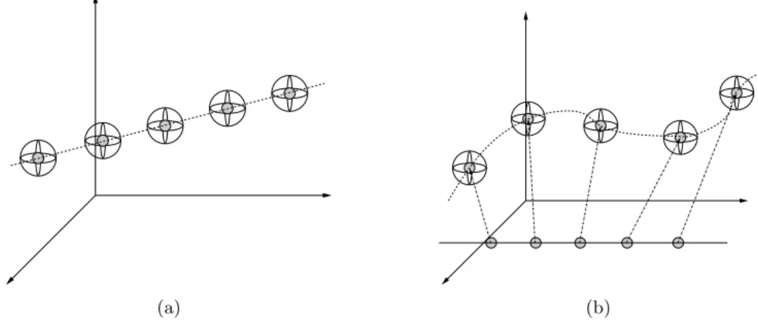
The Generative Topographic Map (GTM) algorithm [Bishop et al., 1998] was introduced as a principled probabilistic analog to SOM. As a generative model GTM realises a “noisy” low dimensional manifold in a high dimensional data space. It can be used to model a given training dataset by adjusting its parameters so that the model-generated data lying around the noisy low dimensional manifold match (in the distribution sense) the training data. GTM is a mixture of local generative models (spherical Gaussians) that adheres to topological constraints (constraints on the values that means of the Gaussians can take). A simple example is that of requiring that the means belong to a straight line. This could be useful if we believed that the data are intrinsically one-dimensional and are adequately represented by a “noisy line”. This situation is illustrated in Fig. 1.1(a). The line on which the means of local Gaussians are placed can be viewed as an image of a one-dimensional interval under a linear (aﬃne) map. Alternatively, one may want to constrain the Gaussian means to lie on a smooth curve. In that case, the one-dimensional interval would be embedded in the high dimensional data space through a smooth non-linear mapping. This is illustrated in Fig. 1.1(b). The GTM belongs to the class of so called latent-variable models with latent space being the one-dimensional interval through which the Gaussian means are constrained.

GTM sets a paradigm of a generative probabilistic approach to the construction of topo-graphic maps. In this work we extend this paradigm to the visualisation of structured data. A substantial part of this work is concerned with developing an extension for tree-structured data that employs hidden Markov tree models as noise models. We compare our approach with a can-didate member of the recursive neural-based techniques, the SOM for structured data (SOMSD) [Hagenbuchner et al., 2003]. This comparison concerns also recursive neural-based approaches in general and serves the purpose of illustrating the beneﬁts of a principled probabilistic model-based formulation. For example, the generative nature of our model formulation provides us with an explanatory insight as to how the data might have been generated. By observing the

(16)

(a) (b)

Fig. 1.1: Spherical Gaussians constrained on a one-dimensional line (a), spherical Gaussians constrained on a one-dimensional curve (b). Note that the straight line (latent space) in (b) does not belong to the data space and is only plotted in the same ﬁgure as its image for convenience. generative process and its parameters we can understand characteristics of clusters of projected data items and/or discern other patterns in the data. Also, the smooth character of the embed-ding map from the latent space into the model space enables us to use techniques of information geometry to characterise areas on the map of potentially clustered data by calculating local ex-pansion/contraction rates in the statistical manifold of local models. Such knowledge is highly desirable for topographic map understanding, but is impossible to obtain in a principled manner from recursive extensions of SOM.

The thesis concludes with the study of a real-world problem. It formulates an extension of GTM that constructs topographic maps of light curves that originate from binary eclipsing stars. To that purpose a probabilistic physical model is formulated.

1.3 Merits of Generative Probabilistic Model-Based

Formula-tions

As aforementioned, this thesis discusses extensions of the GTM to novel data types as well as the beneﬁts of this approach over recursive neural-based extensions of SOM. The beneﬁts of the approach followed here stem from its probabilistic and model-based nature.

Amongst the benefits of generative probabilistic models, is their capability of modelling un-certainty. In such models a function of likelihood arises that quantifies how well a given dataset is modelled (e.g. [Bishop, 1999, Rabiner, 1989]). The likelihood of the model is a precise objec-tive function that allows comparisons of different model-fittings as a result of alternaobjec-tive choices of initialisation, training parameters and training algorithms. Furthermore, testing for

(17)

overﬁt-ting is possible using the robust method of cross-validation which is applicable in most practical settings, when more sophisticated methods are not available. Of course, error (cost/objective) functions and detection of overﬁtting are also available in other machine learning models such as discriminative models. However, one advantage of generative probabilistic models is the capability of directly comparing alternative models that may not belong to the same family.

Moreover, probabilistic approaches can handle missing data in a principled manner as for instance in [Ng et al., 2004] where the EM algorithm is employed. Also, in case overﬁtting is detected, measures for regularisation can be taken to improve the generalisation performance of the model. One possibility is maximum a-posteriori (MAP) estimation by the incorporation of priors on the model parameters. For example the common practice in neural networks of adding a penalty term (proportional to the norm of the weights) for regularisation purposes, is justiﬁed when a probabilistic view is assumed [Bishop, 1996]. Another feature is that such models can naturally form mixture models (e.g. mixture of probabilistic PCA models in [Bishop, 1999], e.g. mixture of hidden Markov models in [Smyth, 1997]) and also composite models such as hidden Markov models with emissions modelled as mixture of Gaussians or hierarchical models (e.g. hierarchical hidden Markov models [Fine et al., 1998]).

Furthermore, generative model based formulations inherently lend themselves to being ex-planatory [Smyth, 1999]; observing the underlying generative process, be it a mixture of Gaus-sians, a hidden Markov model or a probabilistic grammar, provides clues as to how data items arise. This may also inform us on whether the chosen model is a plausible one for a given problem.

1.4 Thesis Organisation

A recurrent theme around the three basic data types of vectors, sequences and tree-structures permeates most of the thesis:

• In chapter 2 we review SOM that processes vectorial data. SOM sets a paradigm that has inspired various extensions that introduce feedback connections to allow for the processing of data expressed as sequences and acyclic-directed graphs (trees are a special subcase of graphs). We also review probabilistic extensions of SOM. A discussion of these approaches follows.

• In chapter 3 generative probabilistic models are reviewed that model the three data types, namely the Gaussian density for vectors, hidden Markov models for sequences and hid-den Markov tree models and Markov tree models for tree-structures. These generative

(18)

probabilistic models are trained via the Expectation-Maximisation algorithm that is also reviewed in the same chapter.

• In chapter 4 the GTM algorithm is reviewed that constructs topographic maps of vectorial data. We brieﬂy mention an extension of GTM, which here we shall refer to as GTM-HMM that processes sequences [Tiˇno et al., 2004], and formulate our own two extensions the GTM-HMTM and GTM-MTM that process tree-structures. Experimental results are presented and analysed. We also discuss the advantages that the generative probabilistic formulation of our approach brings compared to a candidate member of the recursive neural-based approaches.

• Chapter 5 introduces magniﬁcation factors that reveal local contractions/expansions on the topographic map. Magniﬁcation factors are derived for the GTM and the extensions presented in chapter 4. Experimental results are presented and discussed.

• In chapter 6 we depart from the processing of vectors, sequences and tree-structures and demonstrate the power of our generative probabilistic formulation by considering a real world problem. We consider light curves from eclipsing binary stars and derive a GTM3

that constructs topographic maps of such astronomical objects. A probabilistic physical model is formulated and employed as the local noise model for the new GTM. We present the resulting topographic maps and plots of magniﬁcation factors.

• Chapter 7 concludes the thesis with a discussion of its main contributions.

1.5 Thesis Contributions and Publications

This thesis makes the following contributions:

• Develops two novel extensions of the GTM algorithm for the visualisation of tree-structured data, accompanied by a discussion comparing these extensions to a representative of re-cursive neural-based approaches (chapter 4).

• Develops a novel extension of the GTM algorithm for the visualisation of light curves from eclipsing binary stars (chapter 6).

• Studies two approaches for the measurement of magniﬁcation factors in topographic maps (chapter 5). The study is not limited to the extensions of GTM developed in this thesis,

3_{By ‘GTM’ we shall refer both to the GTM algorithm by [Bishop et al., 1998] and to the probabilistic generative}

(19)

but also concerns the original GTM and a previously developed GTM for the visualisation of sequences [Tiˇno et al., 2004].

This work has lead to the following publications:

1. Peter Tiˇno, Nikolaos Gianniotis: Metric Properties of Structured Data Visualizations through Generative Probabilistic Modeling. International Joint Conference on Artiﬁcial Intelligence 2007: 1083-1088.

2. Nikolaos Gianniotis, Peter Tiˇno: Visualisation of Tree-Structured Data through Generative Probabilistic Modelling. European Symposium on Artiﬁcial Neural Networks 2007: 97-102. 3. Nikolaos Gianniotis, Peter Tiˇno: Visualisation of Tree-Structured Data through Generative Topographic Mapping. Submitted to IEEE Transactions on Neural Networks: Accepted subject to minor modiﬁcations.

(20)

Chapter 2

Neural-Based Approaches to

Topographic Mapping

The Self-Organising Map (SOM) [Kohonen, 1990] is the archetypal neural network algorithm for the topographic mapping of vectorial data. SOM has enjoyed considerable success in many diverse areas, a comprehensive array of applications can be found in [Kaski et al., 1998, Oja et al., 2003]. Furthermore, it has inspired numerous extensions that deal with data of non-vectorial types. An excellent overview of such extensions under a general framework can be found in [Hammer et al., 2004]. SOM and its extensions rely on a Hebbian type of learning where two processes, one ofcompetitionand one ofcooperation, take place between the neurons. For the purposes of visualisation, neurons are usually organised on a two dimensional rectan-gular lattice. All neurons are supplied with weight vectors. At every time step a data item is presented to the network and the neuron that is closest to the pattern is declared the winning neuron. This is the competition step. The weights of the winning neuron are updated so as to increase its future activation to this particular pattern. Next at the cooperation step, the weight vectors of neighbouring neurons are also updated, albeit to a lesser extend. This type of training leads to a topographic ordering of the neurons on the lattice. Extensions of SOM to structured data types generally adhere to this framework of learning. However, in order to capture the structure of the particular data type, a notion of context is introduced. Structured data types, such as sequences or graphs, are processed in a recursive manner by adding feedback connections, e.g. a sequence might be processed one symbol at a time and the neural activation induced by each symbol is fed back to the network as complementary to the input of the next symbol. During such recursive processing of a data item, a context is created and recursively updated at each time step that represents the components of the data item processed until the

(21)

current competition step.

For all of the techniques presented in this section we deﬁne here some common notation. In particular each extension to SOM formulates a q-dimensional rectangular lattice of neurons indexed by j = 1, ..., M (q is typically set to 2 for visualisation purposes). The location of a neuron j on the lattice is referenced by a q-dimensional vector xj. Each neuron j is supplied by a weight vector w_j _∈_Rd, wheredis the dimensionality of the input space, and its activation (response) to an inputt is denoted byyj(t).

2.1 Vector Quantisation

Before reviewing SOM, we consider the vector quantisation algorithm (VQ) [Gray, 1984] which may be viewed conceptually as a precursor to SOM. We consider the domain of vectors t_∈Rd. The goal of VQ is dimensionality reduction or data compression. VQ seeks to achieve this by producing a set of M codebook vectors w ∈ Rd, that are suﬃcient approximations of the set of input vectors. In a practical setting, each time a vector t needs to be transmitted via a communication channel, VQ selects the closest codebook w vector, in the Euclidean distance type of sense, and transmits that instead. Provided both ends of the channel share the same codebook, only the index of the codebook needs to be transmitted which procures a gain in communication bandwidth.

VQ deﬁnes an encoding function γ(·) and a decoding function ζ(·). Thus, for perfect encoding-decoding we have that ζ(γ(t)) = t. The distortion, that is the eﬃciency of the encoding-decoding process, can be measured by the mean squared error:

D=

Z

tp(t)kt−ζ(γ(t))k

2_d_t_, _(2.1)

where p(t) is the probability distribution of the data.

The goal is then to adjust the encoding and decoding functions so that the distortion is minimised. Training of VQ proceeds via the generalised Lloyd algorithm [Gray, 1984]:

• Step 1. Given inputt, calculate its Euclidean distance to all codebooks and return the in-dex of the codebook with the minimum Euclidean distance. Thus,γ(t) =argmin_j

kt₋w_j_k2

.

• Step 2. Given codebook indexγ(t) =j, replace codebookwj by the centroid of all vectors that γ would encode as the codebook w_j. Thus, ζ(j) = _|_t_∈{_γ₍1_t₎₌_j_}|P_t_∈{_γ₍_t₎₌_j_}t. Goto step 1.

(22)

2.2 The Original Self-Organising Map

The Self Organising Map (SOM) [Kohonen, 1990] is a neural network that can be used for the visualisation of vectorial data. We denote elements of the domain of vectorial data by

t _∈ Rd. SOM may be viewed as a constrained version of VQ. The constraint is that neurons are topologically ordered so that the spatial location of a neuron bears a relationship to its weight. This means that neurons of “similar” locations on the lattice, have “similar” weights, hence represent “similar” regions of the input space. The constraint is not imposed explicitly but is a consequence of the training algorithm that introduces a lateral interaction between the neurons favouring this organisation. This contrasts with VQ where codebooks are independently updated.

Learning in SOM constitutes of two steps, a competitive step and a cooperative step. SOM alternates between the two steps for each iteration i= 1,2, . . .. Starting with the competition at each iteration i, SOM is presented with a randomly chosen input vectort. The activation of each neuron j is calculated as:

yj(t) =kt−wjk2, (2.2)

which is the squared Euclidean distance between the weight wj of neuronj and the presented input t. A competition is then announced amongst all neurons with the purpose of ﬁnding the best matching neuron to the presented input, i.e. the neuron whose weight has the minimum Euclidean distance to the input. This neuron is declared the winner of the competition and is denoted by I(t): I(t) =argmin j yj(t) . (2.3)

The cooperation step follows, which involves updating the weights of neurons so as to increase their future activation to this particular pattern. This update is conditioned by a neighbourhood deﬁned around the winning neuron as its centre. Neurons in the neighbourhood have their weights updated depending on their distance from the centre of the neighbourhood. Thus, neurons closer to the winning neuron have their weights adjusted closer to the input pattern, than neurons that are more distant. The distance between the winning neuronI(t) and a neuron

j is formally deﬁned by a neighbourhood function h of the type:

h(j, I(t)) = exp(−dist(j, I(t))

σ(i)2 ), (2.4)

wheredist(j, I(t)) is the lateral distance between neuronsjand I(t) (e.g. Manhattan distance), and σ(i) is a parameter that controls the width of the neighbourhood. This distance is

(23)

incorpo-rated in the update rule of the weights. Moreover, a learning rate η(i) is also included to form the following expression for updating the weights of neuron j:

wj(i+ 1) :=wj(i) +η(i)h(j, I(t))(t−wj(i)), (2.5) wherewj(i) is the weight of neuronj at iteration i. The neighbourhood function possesses two important properties; it is symmetric around the winning neuron where d(I(t), I(t)) = 0, and secondly it decreases monotonically. Also since d(I(t), I(t)) = 0, winning neuron I(t) receives the greatest update. The learning rateη and neighbourhood functionh are dependent on time. These parameters adhere to a time-decaying schedule of the type:

η(i) =η0exp(− i η1 ), (2.6) σ(i) =σ0exp(− i σ1 ), (2.7)

where the constantsη0, σ0 deﬁne the initial values for the learning rate and neighbourhood and

constantsη1, σ1 control the rate of decay respectively. The gradual decay ofη andh is essential

for the topographic organisation of the neurons. Repeated presentations of input data, gradually shift the weights of the neurons which eventually approximate the probability density of the data

p(t).

Training of the map continues until the weights of the neurons become stable. SOM with a two (or three) dimensional lattice can be used for visualisation of the input data by projecting each input tto theq-dimensional lattice of neurons. The image of each inputtin the lattice is given by the location vector xof the neuron that produces the greatest activation for input t:

x_←I(t). (2.8)

2.3 Recursive Extensions to the Self-Organising Map

In this section we review some of the representatives of the recursive extensions to SOM for the processing of structured data namely sequences and acyclic directed graphs.

TheTemporal Kohonen Map (TKM) [Chappell and Taylor, 1993] has been designed for the processing of sequences s= [s1,s2, . . . ,sT] over Rd. Each neuron j is equipped with a weight vector w_j _∈ _Rd. At each iteration i, A single input symbol1 s_t, t = 1, . . . , T is processed in a

1_{The use of index}_t_{for symbols of sequences is in potential conflict with the notation of vectors}_t_{. We choose}

(24)

context given by the past activations of the neuron. So neurons in TKM do not lose their past activity immediately as in SOM when a new input is presented, but the context information decays gradually. When the processing of an entire stringshas been completed, the past activity of all neurons is reset to zero. The activation of neuronjat iterationifor inputst, is computed as follows:

yj(st) =αkst−wj(i)k2+ (1−α)yj(st−1), (2.9)

where for the activation yj(s0) we deﬁne thats0=is the empty sequence so that yj() = 0, and α_∈(0,1) is a decay parameter. The winner for input st is:

I(s_t) =argmin j yj(st) . (2.10)

Training at each iterationiinvolves adapting weightwj to the current inputstin the same Hebbian fashion as in SOM, using the following rule:

wj(i+ 1) :=wj(i) +ηh(j, I(st))(st−wj). (2.11) The parameterηis the learning rate andh(·,·) is a Gaussian neighbourhood function deﬁned on pairs of neurons on the map:

h(j, I(s_t)) = exp(−dist(j, I(st))

σ2 ), (2.12)

wheredistis the distance of neuronsjandI(st) on the map andσcontrols the neighbourhood size. Parameters η and σ are decreased with time to allow for topographic convergence as in SOM [Kohonen, 1990].

Recurrent SOM (RSOM) [Varsta et al., 1997] modiﬁes TKM by summing the deviation of the weights wj as opposed to distances. At iteration ithe activation of neuronj for inputstis:

y_j(st) =α(st−wj(i)) + (1−α)yj(st−1). (2.13)

The result of this summation is a vector as opposed to a scalar in TKM and again previous inputs are utilised in a recursive manner. The winning neuron in this case is the neuron that satisﬁes: I(st) =argmin j ky_j(st)k . (2.14)

Here however, adaptation takes into consideration the previous inputs, coded in y_j(i), by

(25)

adapting the weights as follows:

wj(i+ 1) :=wj(i) +ηh(j, I(st))yj(st). (2.15) Recursive SOM (RecSOM) [Voegtlin, 2002] takes into account the context of inputs by ex-plicitly augmenting each unit j with a context vector cj ∈Rq that represents the activations of all the units in the map at the previous iteration. The activation is computed as:

yj(st) =αkst−wjk2+βk[exp(−y1(st−1)), . . . , exp(−yM(st−1))]T −cjk2, (2.16) where α and β are positive constants that control the contribution of the weight and context vectors respectively. Training again is Hebbian for both w_j and c_j:

wj(i+ 1) := wj(i) +η1h(j, I(st))(st−wj), (2.17)

cj(i+ 1) := cj(i) +η2h(j, I(st))([exp(−y1(st−1)), . . . , exp(−yM(st−1))]T −cj),(2.18) whereη1 andη2 are the learning rates for weight and context vector respectively. Thus, neurons

do not compete only in matching their weight vector to the current input, but also their context vector to the current context of the input.

[u , nil , nil ]4 [u , nil , nil ]5

[u , I(4) , I(5) ]3

1 2

4 5 3

Fig. 2.1: Activation for label u₃ of a tree-pattern in SOMSD: Activation is calculated bottom up, thus the children of input node 3 are processed beforehand. Since nodes 4 and 5 are leaf nodes their contexts are ﬁlled in with the special nilvector. The winner neuronsI(4) andI(5) of the input labels u4,u5 of nodes 4 and 5 respectively are supplied as the context for node 3.

Further in the context of sequence processing, the Merge SOM (MSOM) is introduced in [Strickert and Hammer, 2005]. Similarly to RecSOM, each neuron is equipped with a context

(26)

vector cj ∈ Rd. In this case, the context vector cj does not represent the activations of the entire map, but is a combination of the weight and context c_I₍_s_t−1) of the previous winner. The

activation of a neuron j is computed as:

yj(st) =αkst−wjk2+ (1−α)kci−cjk2, (2.19) where ci is the current context and α ∈[0,1] is a parameter that controls the contributions of current input and context. The current context vector is given by the following linear combina-tion:

c_i =βc_I₍_s_t−1)+ (1−β)wI(st−1). (2.20)

At the beginning of the processing of a sequence, the context is set equal toc₁ =0. Training again is Hebbian for both wj and cj, applied at each time step.

SOM for Structured Data (SOMSD)presented in [Hagenbuchner et al., 2003] is an extension of SOM designed to process patterns expressed as directed acyclic graphs (trees and sequences are special cases). Each node v of a graph pattern has a label uv ∈Rd. Each neuron j besides its weight vector wj ∈Rd is supplied with k additional coordinate vectors cj ∈Rq, where k is the maximum out-degree of the graphs in the dataset. Similarly to RecSOM, these additional vectors try to capture the context of the current input. The context is provided by the winning neurons I(j) of children j = 1,2, .., k of the node v currently processed. Thus, each context vector c_j tries to match winning neuronI(j). The augmented input to SOMSD is:

[uv, I(1), I(2), . . . , I(k)]. The activation of neuronj is calculated as:

yj(v) =µ1kuv−wjk2+µ2(kI(1)−c1k2+· · ·+kI(k)−ckk2), (2.21)

where µ1 and µ2 are positive constants that control the contribution of the input label uv and the context vectorsci. Processing of input items proceeds in a bottom-up fashion: before a node

v can be processed all of its children must be already processed. This is illustrated in Fig. 2.1. Therefore, processing starts from the leaf nodes (nodes without children). When a leaf node is processed the context vectors are set to some default values representing the empty treenil. The same applies for nodes with less thank children where the coordinate vectors cj of the missing children are substituted by nil. The coordinate vector of nil is chosen to be (₋1, . . . ,₋1) so that it resides outside the lattice. SOMSD is trained in a Hebbian fashion and as is usual in

(27)

SOM-type formulations, the learning rate and the neighbourhood radius decay gradually. The winner is the neuron with the closest weight and context vectors to the augmented input:

I(v) =argmin j yj(v) . (2.22)

Ifµ1 is set to 1 and µ2 is set to 0, SOMSD reduces to the standard SOM algorithm.

2.4 Probabilistic and Kernel Extensions of the Self-Organising

Map

The approaches presented in the previous section do not use an explicit model for the data and rely on the neural network to develop an internal suitable representation.

In [Hollmén et al., 1999] a Self-Organising Map for Clustering Probabilistic Models is pre-sented, where each neuron stores as its weight a vector wj that contains the parameters of a probabilistic model. Thus, each neuron parametrises a local density p(·|wj). The setting of this study is the exploration of temporal data and more specifically of user-profiles on a mo-bile communications network. User profiles are binary sequences s=_{s1, . . . sT}, st ∈ {0,1} of length T. A call is described as an observed process of transition cases: (st= 0, st−1 = 1) is the

beginning of a call, (st= 1, st−1 = 0) is the end of a call, (st= 1, st−1 = 1) is an on-going call

and (st = 0, st−1 = 0) is on-going silence. The probabilistic model for user-proﬁles is a process

governed by a transition matrix B with entries of probabilities bkl = p(st =l|st−1 = k). The

sum of entries of matrix B of each row must equal to 1. The model instantiated by neuronj is:

p(s_|wj) = T Y t=1 p(st=l|st−1 =k,wj), logp(s|wj) = T X t=1 logp(st=l|st−1 =k,wj). (2.23) The log-likelihood in (2.23) is used to determine winner I(s) for input s presented at the competition step: I(s) =argmax j T X t=1 logp(st=l|st−1 =k,wj) , (2.24)

The log-likelihood in (2.23) is also used in the adaptation rule:

wj(i+ 1) :=wj(i) +ηh(j, I(s))

d dwj

(28)

where neighbourhood function hand the learning rateη are reused from (2.4) and (2.6) respec-tively. Note that this update rule can lead to invalid parameters (parameter are probabilities which must be restricted in [0,1]). Thus, measures in the form of a suitable parametrisation or constraints must be taken. In [Hollm´en et al., 1999] the solution of introducing a suitable parametrisation is used.

In [Kaski et al., 2001] a SOM formulation is presented in the setting of bankruptcy analysis, where the winner neuron is determined by a distance metric based on the Fisher information matrix. Even though this approach is concerned with vectorial data, it is of interest since its aim is to use a data-driven metric instead of the customary Euclidean distance metric. The data are ﬁnancial statements of companies and are pairs of feature vectors t _∈ _Rd, describing certain indicators such as growth, proﬁtability etc. of a company, and binary indicator variables

c_{∈ {}0,1_} signifying the bankruptcy risk of the company in the next three years. The goal is to achieve a topographic organisation of the datatdriven by the implicit information present inc

that indicates which features are relevant to the task of bankruptcy risk analysis. A prediction of bankruptcy risk for a statement t, is expressed as a conditional density p(c|t) which is (as in many other application domains) unknown. The joint density p(c,t) is learnt from the data, and the conditional densityp(c|t) is then obtained via Bayes’ rule.

Small displacements in the conditional density, i.e. p(c_|t+dt), reveal how variablecchanges depending on the directionsdt. Such small changes can be measured by the KLD, which locally is:

DKL[p(c|t)||p(c|t+dt)] =dtTF(t)dt, (2.26) whereF(t) is the Fisher information matrix evaluated att, that reveals local scaling factors. On the SOM lattice, each neuron j is equipped with a weight vector wj ∈ Rd. The weight vector parametrises a local conditional density p(c|wj). When SOM is presented with input t

at competition step, winner I(t) is determined by:

I(t) = argmin j DKL[p(c|wj)||p(c|t)] = argmin j dtTF(wj)dt , (2.27)

wheredtis the Euclidean distance betweenwjandt. The metric in (2.26) should strictly be used for computing local distances within the neighbourhood of a neuronj, while non-local distances should be calculated as path integrals. However, the same metric is also used to approximate non-local distances by assuming that it will be locally accurate and that neighbours with a

(29)

greater separating distance dt will still be calculated as being farther than close neighbours. Thus, the winner should still be determined accurately. Although the winner is determined by metric (2.26), the update rule for the weights is the same as in the original SOM.

An interesting approach is undertaken in [Verbeek et al., 2005] where Self-organising mix-ture models (SOMM) are developed. The core idea of the approach is that a topology can be introduced into a mixture model, by modifying the E-step of the EM algorithm. The approach can be extended to any probabilistic model that can be optimised via EM, hence various data types can be accommodated. Here we consider vectors t and a mixture model of C Gaussian componentsp(t(n)_|θc): p(t|Θ) = C X c=1 p(c)p(t(n)|θj), (2.28) whereΘencapsulates vectors θj, the parameters of the individual Gaussian components. Each component j is associated with a coordinate vectorxj which for visualisation purposes is two-dimensional. Coordinate vector xj determines the position of the component in a latent space that will be used to project the high-dimensional dataset. To that purpose coordinate system

x is deﬁned as a rectangular grid in the latent space.

When using EM to train a mixture of Gaussians, in the E-step the posterior distribution of the components is estimated. The posterior may be factorised for independently generated data, and we denote the posterior distribution concerning the n-th data item by p(j|t(n)). The posterior is used in the M-step to weigh the contribution of each data item t(n) in updating the parameters of each component j (for more details see 3.2.1). Intuitively, posterior p(j|t(n)) expresses the responsibility that component j bears for generating data item t(n). In SOMM, the E-step is modiﬁed in order to introduce a sense of topology. Viewing posteriorsp(j_|t(n)) as functions of components j, we restrict them to smooth, normalised distributions of the form:

hk(j)∝exp(−σkxk−xjk2), with M

X

j=1

hk(j) = 1, (2.29) where k= 1, . . . , C is an index over components and σ controls the radius of the distributions. Each distributionhkis centred at a componentkand acts as a neighbourhood function similarly to the one deﬁned in SOM. In the modiﬁed E-step, for each inputt(n) we choose a neighbour-hood functionhk that minimisesDKL[hk||p(j|t(n))] as the posterior probability given t(n). This introduces a lateral interaction between the mixture components when it comes to updating the parameters in the M-step; forp(j_|t(n)) =hkcomponentkreceives the most responsibility, while neighbouring components also receive responsibility, albeit to a lesser degree.

(30)

In the setting of Gaussian mixtures, the E- and M-step translate to the following update equations: 1. E-step: p(j_|t(n)) =argmin_h_k DKL[hk||p(j|t(n))]

2. M-step: Perform standard M-step, using the posteriors from modiﬁed E-step.

Parameterσmay be annealed from a wide neighbourhood function to a small neighbourhood with an appropriate schedule. Once training has been completed, each data pointt(n)is mapped to the latent space as the mean of the posterior distribution over the latent space:

proj(t(n)) = C

X

j=1

p(j_|t(n))xj. (2.30) In [Hofmann, 2000]ProbMap is introduced, which constitutes a probabilistic approach to vi-sualising document collections. ProbMap learnsK(Kis a parameter of the algorithm) thematic topics from a document collection and organises them on a two-dimensional lattice so that neigh-bouring topics are similar. Each neuron indexed by k= 1, . . . , K on the SOM lattice represents one of theK topics to be learnt. A dataset of documents is a setD={d(1), ..., d(N)}, whered(n)

with 1_≤n_≤N is a document. Each document consists of T(n) number of words from a ﬁxed vocabulary V ={w1, ..., wR}, thus d(n) = (d(₁n), . . . d(_Tn₍)_n₎) with dt(n) ∈V. Each document d(n) has a parameter vector of probabilities τn= [p(1_|d(n)). . . p(K_|d(n))], where p(k_|d(n)) quantiﬁes the degree to which document d(n) _{expresses thematic topic} _k_{, with} PK

k=1p(k|d(n)) = 1. Also,

for each topic k a parameter vector of probabilities φk = [p(w1|1). . . p(wR|K)] is deﬁned where

p(wr|k) expresses the probability that word wr occurs under topic k, with PR_r₌₁p(wr|k) = 1. A ﬁxed, symmetric neighbourhood function is imposed on the SOM lattice that returns the distance between two neuronsk andl:

p(l|k) = exp(−σ h(k, l) 2₎ PK l′ =1exp(−σ h(k, l′)2) , (2.31)

whereσ controls the radius of the neighbourhood andh(k, l) is the Euclidean distance between neuronsk and lon the lattice. Thus, a distance is imposed on theK topics to be learnt.

ProbMap is a generative model operating as follows. A documentd(n) _{is produced by}

gen-erating one word d(_tn) at a time. For each t = 1, . . . , T(n) a random topic k is chosen with probability p(k_|d(n)). Chosen topic k is corrupted with a probability p(l_|k) into a second topic

l. However, the nature of p(l|k) is such that a topic is more likely to be corrupted into a topic represented by neurons close to neuronk than into a topic represented by neurons distant tok.

(31)

This introduces the topographic organisation of the topics. Having chosen the second topicl, a word for d(_tn)=wr is generated with probability p(wr|l).

The model likelihood given dataset _Dreads:

L(τ, φ|D) = N Y n=1 K X k(₁n)=1 K X l(₁n)=1 · · · K X k_T(n₍)_n₎=1 K X l(_Tn₍)_n₎=1 T(n) Y t=1 p(k(_tn)|d(n))p(l(_tn)|k(_tn))p(d_t(n)|l(_tn)),(2.32) where vectors k(_tn) and l_t(n) refer to the topics responsible for generating the word d(_tn). The model likelihood is maximised via the EM algorithm by postulating a set of hidden variables that indicate which states were responsible for the generation of each word. Adjusting parameters τ

and φ in this framework leads to an organisation of K thematic topics on the two-dimensional lattice.

Departing from the probabilistic extensions of SOM, in [Andr´as, 2002] SOM is modiﬁed to incorporate a kernel function in calculating activations of neurons. A kernel function is a function

K that calculates the inner product K(t,t′) =F(t)T_F₍_t′_{) of data items}_t_∈_Rd _{embedded in a} high dimensional spaceRd′ (d′ > d), via a function F :Rd→Rd′ that transforms the originally linearly inseparable dataset into a linearly seperable dataset. Although, topology preservation is important here, the introduction of a kernel function aims to improve the classiﬁcation ability of SOM: a trained SOM may be used for classiﬁcation by assigning each data item t the class of the closest neuron j, i.e. class(t) =class(argmin_j

yj(t)

).

As stated in [András, 2002], SOM learns a Voronoi tessellation of the data space, which in the case of a linearly inseparable dataset is a difficult task that requires a large lattice (i.e. high number of neurons) in order to learn an accurate topographic map. However, if the data are linearly seperable the task is easier and a smaller lattice suffices. The activation of a neuron

j given transformed data item F(t) is yj(t) = kF(wj)−F(t)k2, where weights w are also embedded into Rd′. We may rewriteF in terms ofK:

yj(t) =kF(wj)−F(t)k2 = (F(wj)−F(t))T(F(wj)−F(t))

= F(t)TF(t) +F(w_j)TF(w_j)−2F(t)TF(w_j)

= K(t,t) +K(w_j,w_j)−2K(t,w_j). (2.33) Hence, the winnerI(t) is determined by:

I(t) =argmin j K(t,t) +K(wj,wj)−2K(t,wj) . (2.34)

(32)

Also the update rule is formulated as: wj(i+ 1) := wj(i) +ηh(j, I(t)) ∂ ∂wyj(t) := wj(i) +ηh(j, I(t))( ∂ ∂wK(wj,wj)− ∂ ∂w2K(t,wj)). (2.35)

Of course one must choose the form ofK. In [Andr´as, 2002] the kernel function K(t,t′) =

K(t,t′;ω) is parametrised by parameter vectorωwhich allows the adaptation of the kernel. The learning of the kernel function is supervised and is performed via the LVQ algorithm. Once SOM has been trained, the neurons are labeled e.g. by the majority class of data items in Voronoi cell of the neuron. Parameters ωare set so that the best classiﬁcation labels for the neurons are found. Adapting parameter ω changes the the boundaries of the Voronoi cell and consequently the membership of data points to the Voronoi cells in directions that better classiﬁcations may be obtained.

In [Günter and Bunke, 2002] SOM is extended to work with data expressed as graphs. The neuron associated weightsware no longer feature vectors (codebooks) but explicit graph repre-sentations. Since graph data are not expressed in the convenient form of vectors, one must define a suitable distance function that measures affinities between data vectors and the representa-tions stored in the neurons of the lattice, and also formulate an update rule that decreases the distances between data vectors and representations in neurons. The first requirement is satisfied by employing the graph edit distance dedit which is defined as the least number of operations that are necessary to transform a graphginto a graphg′. Edit operations include the insertion, deletion or relabelling of a node or edge. Thus, the less operations needed to transformg into

g′, the less the distancededit(g,g′) between them. Moreover, edit operations are associated with non-negative cost values. This makes the graph edit distance more robust to distortions (noise) present in graph data (e.g missing edges or nodes) by typically assigning low costs to the edit functions that remedy the most frequent type of distortions. The winner neuron is deﬁned as:

I(g) =argmin j dedit(g,wj) . (2.36)

By applying only a subset of the necessary edit operations that transform completely graph

gso that dedit(g,g′) = 0, we obtain a graphgofor whichdedit(g,g′) =dedit(g,go) +dedit(go,g′). A function f is deﬁned that for a given distance awith 0_≤a_≤dedit(g,g′), it returns a graph

f(a,g) = go such that the distance dedit(g,go) approximates a as closely as possible. This is useful for the update rule that needs to update the neurons in varying degrees for a given input

(33)

data item. The update for a neuronj is:

wj :=f(a,g), (2.37)

where a must relate to a decreasing learning rate η and the distance on the lattice h(j, I(g)). Neurons may be initialised by assigning to wa perturbed subset of the training data.

2.5 Discussion of Reviewed Extensions

Although, the recursive extensions of SOM have shown good results in various experimental settings, they are challenged by certain theoretical problems. Neighbourhood preservation is an important property of a good topographic map. It refers to the property of data points maintaining their neighbours after projecting them into the low-dimensional visualisation space. A map may sustain defects such as violations in neighbourhood relations or abrupt discontinuities when a neuron appears to be signiﬁcantly diﬀerent to its neighbouring neurons. Of course alteration of certain neighbourhood relations is inevitable since the reduction in dimension results to a loss of certain topographic information. SOM and its recursive extensions rely on Hebbian learning that does not explicitly optimise a certain neighbourhood preservation criterion. Thus, apart from visually inspecting a map, judging objectively the quality of the achieved topographic organisation is not straightforward.

Numerous suggestions of such quality measures have been put forward in the related litera-ture. For example, quantisation error [Pölzlbauer, 2004] is a measure of how well the input pat-terns match their winning neurons (in a Euclidean sense of distance). However, such a measure does not respect topological aspects of the map. Another is topographic error [Pölzlbauer, 2004], that does take into consideration the topology, but in a restricted way. Topographic error tests whether for an input item the first and second best matching neurons are adjacent on the SOM lattice. If they are, then the mapping is locally continuous, otherwise a discontinuity occurs. Another example of such measures is the topographic product [Bauer and Pawelzik, 1992]. The method measures distances of neurons on the lattice of the map and in the data space (weight space). The intuition is that neurons with similar weights are neighbours in the data (weight) space and for a topographically organised map such neurons should also be neighbours on the lat-tice. The topographic product is concerned with preserving the relative ordering of neighbours, instead of the absolute distances that separate them. Violations in the relative ordering signify topographic defects. Furthermore in [Venna and Kaski, 2001], two measures are proposed for two types of error: neighbourhood preservation addresses the issue of a data point maintaining

(34)

its neighbours in the data space also after projection on the lattice, and trustworthiness refers to the error made when data points that are mapped close to each other on the map are in fact quite dissimilar.

Such criteria deﬁne a certain basis for evaluating topographic preservation of maps obtained by SOM and its extensions (for static data). Even though they do capture certain desirable properties of topographic preservation, we note that they are not related to some kind of ob-jective that guides the optimisation of SOM. Therefore it is inappropriate to use these criteria in evaluating a trained map, since the map is not trained toward yielding favourable values according to the criteria. One can of course evaluate the topographic map at each iteration during training according to some criterion of topographic preservation and stop the training if no further progress (or degradation of the criterion) is observed. However, still in this case, it is not clear that SOM’s Hebbian-type of training should monotonically increase the quality criterion at hand; maybe certain steps that appear counter-productive according to the criterion are necessary in order for the map to ﬁt the data.

The problems above are related to the fact that SOM and its extensions do not formulate an objective function that quantifies the level of topographic ordering of the concerned maps, that could be used in training the maps. The SOM algorithm [Kohonen, 1990] does not explicitly state what is being optimised. Strictly speaking, it is proved in [Erwin et al., 1992] that the update rule of SOM does not constitute a gradient of any objective function. Nevertheless, in [Heskes, 1999] a slight variant of SOM is introduced that does possess such an objective function. The modification simply redefines the winning neuron as:

I(t) =argmin j M X k=1 h(j, k)kt₋w_k_k. (2.38) Hence, the winner in this variant is not simply the neuron closest to the current input, but the neuron that minimises the quantisation error in the local neighbourhood. The form of the update rule remains the same, taking into account that the winner is given by (2.38). This idea of the winner neuron minimising quantisation error in the local neighbourhood, was used in [Hammer et al., 2004] to derive a cost function for recursive neural-based approaches. Computing such a cost function involves computing the activations of the neurons for the given input. Optimising the cost function can then be used to update the weights of the network. However, updating the weights so that the future activations of neurons match the input closer, has an additional eﬀect; changing the activations, changes the cost function. Thus, a cycle is introduced: the cost function depends on the activations of the neurons, and the neurons are

(35)

updated according to the cost function in order to achieve better activations for the inputs. Thus, we are not faced with an ordinary optimisation problem, but something more complex that is difficult to interpret. Note, that this is not the case in SOM: in SOM an immutable Euclidean metric is defined to calculate neuron activations. Therefore, the cost function in [Heskes, 1999] does not suffer from this problem.

Another limitation of the SOM paradigm, mentioned in [Bishop et al., 1996], is that no density model is provided for the data. This deems the treatment of new incoming data items, after training has been completed, problematic. In SOM the location of a new item may be predictable, since we expect it to be placed closed to neurons of weights similar to the input in the Euclidean sense. In recursive neural-based approaches, discussed in section 2.3, the neural dynamics that dictate the placement of a new point are not as easily understood. In these approaches the input is augmented by a context, the formation of which is not easily interpreted. In SOM it is understood what it means to compare an input data item to the weights of neurons and why updating neurons of high response is beneﬁcial. In recursive approaches two comparisons take place when presenting an input to the network. Again, as in SOM, the actual input is compared to the weights of neurons, but also the context of the augmented input is compared with the context of the augmented weights. The signiﬁcance of comparing the contexts and updating them in a Hebbian way, is not easily understood as for example in the case of RecSOM in (2.16) and (2.18).

In connection to the difficulty of understanding projections, recursive neural-based ap-proaches do not to define (at least not explicitly) a clear notion of data similarity. As afore-mentioned, they rely on the training process to form appropriate internal representations that capture data similarities, and this in an unsupervised setting. Thus, recursive neural-based ap-proaches are faced with solving two tasks at the same time without external guidance: evolve an appropriate notion of similarity while striving for topographic organisation. For example, SOMSD is capable of processing graph-structured data as well as trees and sequences. These three data types can be viewed as special subcases of each other, i.e. sequences are trees with outdegree equal to one, and trees are directed-acyclic graphs where each node has a single par-ent. However, if we were to construct a topographic map via SOMSD on a mixed dataset of graphs, trees and sequences, it would be difficult to understand the learnt distance metric. The absence of a notion of similarity makes it difficult to understand what the distances between projected data points on topographic maps constructed by recursive approaches mean. It is not clear whether distances between the projected points on the map can be measured accord-ing to some criterion, and whether this criterion constitutes a proper metric that satisfies the

(36)

triangle inequality. Furthermore, depending on the nature of the problem, various similarity notions may be appropriate, even within a single data type. Interpretation of data is of course problem dependent and datasets of the same data structure may require a diﬀerent similarity interpretation.

This brings us to the next point, that recursive neural-based approaches do not allow any expressive control over the notion of data similarity to the user. This is important because data similarity drives the organisation of the map. SOMSD does provide some control via parameters

µ1 andµ2 regarding the contribution of labels and context. However, if hypothetically we were

interested in sequences whose middle part (or alternatively their prefix or suffix) we knew was more important than the rest of the sequence in judging similarity, the necessary modifications to impose this are not obvious. It seems that such requirements cannot be easily accommodated. The probabilistic extensions to SOM mentioned in section 2.4 seem to alleviate certain problems. In the Self-Organising Map for Clustering Probabilistic Models [Hollmén et al., 1999], a similarity metric is clearly defined in (2.23) that is also used in determining the winning neuron. Neurons in this approach instantiate probabilistic models, the generative nature of which clearly explains why a data item is assigned to its location. However, the update rule in (2.25), fashioned after the update rule in SOM (2.5), seems to be problematic to a certain extent. The goal of the update rule, as interpreted in SOM, is of course to update all neurons in the neighbourhood so that the likelihood-response of each neuron to the current input is increased in the future. After such an update, the winner neuron should remain the winner neuron for the current input since it receives the greatest update after all. Although this is indeed the case in SOM, it is not necessarily in this setting for two reasons. Firstly, in this extension we update the weight of a neuron wj, that parametrises a probabilistic model, with a gradient rule. Thus, if the step size taken in the update rule in the direction of the gradient is inappropriate, it could happen that the likelihood of a neuron would decrease instead of increase. Also, this could result in the likelihood of the winner neuron becoming less than the likelihood of one of its neighbouring neurons regarding the current input. Secondly and more importantly, the weights of neighbouring neurons may be quite different to each other and thus the parametrisation of their induced probabilistic models may differ (due to random initialisation perhaps). This means that the gradients in the update rule, are optimising different regions of the parameter space of the probabilistic model. The current learning rate and value of the neighbourhood function may then have a considerable effect on the adaptation of the likelihoods. Neighbouring neurons with different parametrisation may not express statistically similar density models. On these two accounts, the update rule in (2.25) does not appear to enforce a strict topological ordering