Mathematics Theses Department of Mathematics and Statistics
Summer 8-7-2010
Cox Model Analysis with the Dependently Left
Truncated Data
Ji Li
Georgia State University
Follow this and additional works at:https://scholarworks.gsu.edu/math_theses Part of theMathematics Commons
This Thesis is brought to you for free and open access by the Department of Mathematics and Statistics at ScholarWorks @ Georgia State University. It has been accepted for inclusion in Mathematics Theses by an authorized administrator of ScholarWorks @ Georgia State University. For more information, please [email protected].
Recommended Citation
Li, Ji, "Cox Model Analysis with the Dependently Left Truncated Data." Thesis, Georgia State University, 2010. https://scholarworks.gsu.edu/math_theses/88
by
JI LI
Under the Direction of Xu Zhang
ABSTRACT
A truncated sample consists of realizations of a pair of random variables (L, T) subject to the constraint that L ≤T. The major study interest with a truncated sample is to find the marginal dis-tributions of L and T. Many studies have been done with the assumption that L and T are inde-pendent. We introduce a new way to specify a Cox model for a truncated sample, assuming that the truncation time is a predictor of T, and this causes the dependence between L and T. We de-velop an algorithm to obtain the adjusted risk sets and use the Kaplan-Meier estimator to esti-mate the Marginal distribution of L. We further extend our method to more practical situation, in which the Cox model includes other covariates associated with T. Simulation studies have been conducted to investigate the performances of the Cox model and the new estimators.
INDEX WORDS: Truncation time, Dependent, Marginal distribution, Cox regression model, Kaplan-Meier method, Bootstrap method
by
JI LI
A Thesis Submitted in Partial Fulfillment of the Requirements for the Degree of Master of Science
in the College of Arts and Sciences Georgia State University
Copyright by Ji Li 2010
by
JI LI
Committee Chair: Dr. Xu Zhang
Committee: Dr. Jiawei Liu
Dr. Gengsheng Qin
Dr. Yichuan Zhao
Electronic Version Approved:
Office of Graduate Studies College of Arts and Sciences Georgia State University August 2010
ACKNOWLEDGEMENTS
It is a pleasure to thank all those people who helped me for my research and thesis. First, I am heartily thankful to my supervisor, Dr. Zhang. During the research time with her, I have been consolidating my statistical knowledge and improving my SAS skills. This the-sis cannot be accomplished without her direction and help. Dr. Zhang’s enthusiasm and attitude in doing the research also impacts me. She pays attention to the every detail problem and always tries the new method. With her patient direction and valuable suggestions, finally I can finish my thesis step by step.
I would like to express my gratitution to Dr. Mei-Jie Zhang at Medical College of Wis-consin. He provided me the data source and also gave me many valuable suggestions for my the-sis and my future studies.
I would like to thank Dr. Jiawei Liu, Dr. Gengsheng Qin and Dr. Yichan Zhao who would like to be my thesis committee members. Thanks for their time to read my thesis and gave me helpful comments.
Finally, I am indebted to my family and many of my friends who gave me encouragement and supports during this time.
TABLE OF CONTENTS
ACKNOWLEDGEMENTS ... iv
TABLE OF CONTENTS ... v
LIST OF TABLES ... vii
LIST OF FIGURES ... viii
CHAPTER 1 INTRODUCTION ...1
CHAPTER 2 METHODOLOGY REVIEW ...7
2.1 Kaplan-Meier Estimator ...7
2.1.1 The Kaplan-Meier Estimator for a Right Censored Sample ...7
2.1.2 The Kaplan-Meier Estimator for a Truncated Sample ...8
2.2 The Cox Model ...9
2.2.1 The Cox Model for Right Censored Data ...9
2.2.2 Left –Truncated Version of Cox Model ... 10
2.3 Tsai’s Kendall’s Tau Test to Test the Independence Between T and L ... 11
CHAPTER 3 NEW METHODOLOGY ... 14
3.1 New Regression Model Specification ... 14
3.2 Estimation of the Covariate Effects on the Failure Time ... 15
3.3 Estimation of the Distribution of the Truncation time ... 18
3.3.1 The Truncation Time is the Only Predictor for the Failure Time ... 19
3.3.2 Other Predictors for the Failure Time Exist ... 20
CHAPTER 4 SIMULATION STUDIES ... 23
4.1 The Simulation Study for Model (3.2) ... 23
4.2 The Simulation Study for Model (3.3) ... 28
CHAPTER 5 EXAMPLES ... 33
5.1 Data Description... 33
5.2 To Estimate the Treatment Effect and the Effects of Other Predictors ... 34
5.3 To Estimate the Distribution Function of the Transplant Time ... 37
CHAPTER 6 CONCLUSIONS ... 41
LIST OF TABLES
Table 4.1 Simulation result on the effect of truncation time for Model (3.2) ... 26
Table 4.2 Simulation result on regression coefficient estimation for Model (3.3) with a continuous covariate ... 30
Table 4.3 Simulation result on regression coefficient estimation for Model (3.3) with a discrete covariate ... 30
Table 5.1 Regression coefficient estimates for the Cox model on the pooled sample ... 36
LIST OF FIGURES
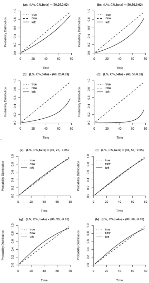
Figure 4.1 L is the only predictor of T ... 27
Figure 4.2 Continuous covariates of T are present ... 31
Figure 4.3 Discrete covariates of T are present ... 32
Figure 5.1 Estimated cumulative hazard rates Chemotherapy group and BMT group ... 37
Figure 5.2 Estimated distribution function of transplant time ... 39
Figure 5.3 90% percentiles confidence intervals for BMT bootstrap samples ... 40
CHAPTER 1 INTRODUCTION
Truncation appears if a continuous random variable T is only observable when it is not
smaller than a truncation variable L. For the truncation examples within the scope of life sciences,
the random variable T is often the time to failure event. The truncation variable L is the entrance
time indicating that the subject enters the study. As a consequence, truncation is also known as
late entrance (Kaplan-Meier, 1958). Let F(t) and G(t) be the distribution functions for T and L,
respectively. The aims of many studies with truncated samples were to estimate the marginal
dis-tribution of F(t) and G(t).
A truncated sample contains n replicates of paired random variables (T, L) subject to the
con-straint L≤T. The well-known Kaplan-Meier estimator is widely adopted to estimate the survival
function of the failure time with right censored data. Kaplan-Meier (1958) clearly mentioned in
their paper that the proposed nonparametric estimator can handle late entrance. One just needs to carefully construct the risk sets. Suppose the events occur at N distinct times 𝑡(�) < 𝑡(�) <⋯< 𝑡(�), 𝑋� =𝑚𝑖𝑛 (𝐶�,𝑇�), 𝐶� is the censoring time. One subject in the sample should be counted in
the risk set at 𝑡 if this subject is associated with the entrance time smaller than t and the failure
time greater than t. According to Kaplan-Meier (1958), as well as Lynden-bell (1973), the
𝐹�(𝑡) = 1− � �1−𝑑�𝑡(�)�
𝑅�𝑡(�)��, 0≤ 𝑡 ≤ 𝜏, (1.1)
�:�(�)��
where 𝑑(𝑡) =∑����𝐼(𝑋� =𝑡,𝛿� = 1), 𝑅(𝑡) =∑����𝐼(𝐿� ≤ 𝑡 ≤ 𝑋�). Suppose 𝑙(�) < 𝑙(�) <
⋯< 𝑙(�) are distinct truncation times. Considering the reversed time axis, one can easily see that
G(t) can be similarly estimated as F(t). Thus, the Kaplan-Meier estimator of G(t) is given by, 𝐺�(𝑡) =� �1−𝑆�𝑙(�)�
𝑅�𝑙(�)��, 0≤ 𝑡 ≤ 𝜏, (1.2)
�:�(�)��
The asymptotic properties of𝐹�(𝑡) have been studied by Woodroofe (1985), Wang, Jewell and
Tsai (1986), Lin and Ying (1991), as well as Keiding and Gill (1990).
All aforementioned works assume the independence between T and L. However, the
in-dependence between failure time variable and truncation time variable needs to be carefully
ex-amined. Tsai (1990) explained that the independence between T and L cannot be
nonparametri-cally verified in the quadrant T<L. To establish the estimator and asymptotic properties, only
in-dependence of T and L in the region T>L is needed. Let 𝐻(𝑡,𝑙) be the joint distribution of T and
L given the condition L<T, the independence condition required in the aforementioned
re-searches is
𝐻�:𝐻(𝑡,𝑙) =
∬∆(�,�)𝑑𝐹(𝑢)𝑑𝐺(𝑣)
𝛼 ,
where 𝛼 =∬ 𝑑𝐹��� (𝑢)𝑑𝐺(𝑣), ∆(𝑡,𝑙) = {(𝑢,𝑣)|𝑢 ≤ 𝑡,𝑣 ≤ 𝑙,𝑢 ≥ 𝑣}. The independence of T and L in the region can be observed is called quasi-independence in the contingency table
litera-ture. Tsai (1990) also proposed a conditional Kendall’s Tau test to test the quasi-independence
for a truncated sample.
Many problems related with a truncated sample emerged in real-life applications and
have been tackled by statisticians. Among these problems, regression analysis on the failure time
T based on a truncated sample has been identified to be practically important. The solution to this
problem is simple if T and L are independent. For the hazard-based regression models, the only
modification one needs to implement in estimation procedure is to use the truncation time to
ad-just the risk set. Regression coefficient estimation for a Cox model is available in some statistical
packages such as SAS and S-plus. Other hazard-based regression models like Aalen’s model or
Lin and Ying’s model can be similarly implemented by properly constructing the risk sets.
Regression model with a truncated sample is practically needed in Bone Marrow
Trans-plant (BMT) studies. Leukemia patients can be treated with chemotherapy and Bone Marrow
Transplant. Due to the complication in finding matched donors and ethical considerations, the
large-scale randomized trial with these two treatment arms is not practically feasible. The
solu-tion is to pool together different sources of data. The Internasolu-tional Bone Marrow Transplant
Re-gistry (IBMTR) is the primary source of BMT cases. Data on patients receiving chemotherapy
have been collected by some research groups or institutions, such as the Pediatric Oncology
or leukemia relapse is the response variable. The data collected from chemotherapy group is a
right-censored sample. However, the BMT cohort includes only the transplant cases, and the
pa-tients who died before the matched donors and be identified are excluded.It is necessary to treat
the BMT cohort as a truncated sample. Klein and Zhang, (1996) used a left truncated version of
the Cox model on the simulated data and had a satisfactory result. The left truncated version of
Cox model has been used as the standard method in quite a few pooled-sample studies. However,
their methods assume the same baseline between chemotherapy group and BMT group. Let L be
the transplant time. The conditional proportional hazards model for BMT group has the form: 𝜆(𝑡|𝐿) =� 𝜆�(𝑡)exp(𝛽�+𝛼�𝑧) if 𝑡 <𝐿
𝜆�(𝑡)exp(𝛽�+𝛼�𝑧) if 𝑡 ≥ 𝐿
where exp(𝛽�) is pre-transplant differences between two treatments, exp(𝛽�) is the
post-transplant hazard ratio between treatments, and 𝜆�(𝑡) is the hazard rate function for
chemothera-py group. Note that 𝛽� in the above model is a nuisance parameter and is unestimable with the
pooled samples. The common baseline hazard assumption is legitimate in a randomized trial
set-ting in which patients in BMT group are treated by chemotherapy before they receive transplants.
However, this assumption is strong when the pooled samples are used, whereas the study cohorts
are collected from very different geographical locations and probably different time frames. For
this approach, the effect of transplant is assumed to be constant. It has caught attentions in
waiting time cannot be evaluated within this framework. These drawbacks reveal the limitation
of this analytical approach.
Estimation of the marginal distributions of T and L is rarely studied for a dependently
trun-cated sample. We conducted online search on this topic and found only one work by Emma and
Konno (2009). To tackle this issue, Emma and Konno used a bivariate normal distribution to
model a dependently truncated sample. The marginal distribution of T and L are governed by the
assumed joint distribution. The maximum likelihood estimation method was used to find the
es-timates of the parameters in the bivariate normal distribution. It is not clear how Emma and
Konno’s method can be extended to the context that the failure time is associated with multiple
predictors.
In this study, we proposed a regression model with new model specification to analyze the
dependently truncated sample. The truncation time is treated as a covariate in a Cox model to
describe the dependence between L and T. The left-truncated version of Cox model is used to
assess the effects of truncation time and other covariates on the failure time. We propose an
algo-rithm to obtain the adjusted risk sets and a Kaplan-Meier estimator to estimate the marginal
dis-tribution of L. In Chapter 2, we briefly describe the Kaplan-Meier estimator and the Cox
regres-sion model for right censored samples and independently truncated samples. In Chapter 3, we
simula-tion study. Chapter 5 uses the BMT data example to illustrate the proposed method. The
CHAPTER 2 METHODOLOGY REVIEW
2.1 Kaplan-Meier Estimator
2.1.1 The Kaplan-Meier Estimator for a Right Censored Sample
Kaplan-Meier estimator, also known as the product-limit estimator, is the routine
estima-tion method for the survival funcestima-tion for right censored failure time data. Suppose the events oc-cur at N distinct times 𝑡(�) < 𝑡(�) <⋯ <𝑡(�), and at time 𝑡(�) there are 𝑑(𝑡(�)) events. Let R(t) be
the number of individuals who are at risk at time 𝑡, that is 𝑅(𝑡) =∑����(𝑋� > 𝑡). The
Kaplan-Meier estimator for the survival function of the failure time is given by 𝑆�(𝑡) =∏ �1− �(�(�))
�(�(�)) �
�: �(�)�� , 0≤ 𝑡 ≤ 𝜏, (2.1) where𝜏 is the largest failure time. The Product-limit estimator is a step function with jumps at
the observed event times. The size of these jumps depends not only on the number of events ob-served at each event time 𝑡(�), but also on the pattern of the censored observation prior to 𝑡(�).
The variance of this Product-Limit estimator can be estimated by the Greenwood’s formula,
𝑉��𝑆�(𝑡)�=𝑆�(𝑡)� � 𝑑(�)
𝑅(𝑡(�))(𝑅(𝑡(�))− 𝑑(�))
�:����
2.1.2 The Kaplan-Meier Estimator for a Truncated Sample
For a truncated sample, the truncation time 𝐿� is also observed for the jth subject and 𝐿� < 𝑋�. For the pair (𝐿�,𝑋�), 𝐿� is the time when he/she enters the study and 𝑋�is the time when
he/she dies or censored. We redefine R(t)as the number of individuals who entered the study
prior to time 𝑡 and remained under study at t , then 𝑅(𝑡) =∑����𝐼 (𝐿� ≤ 𝑡 ≤ 𝑋�).
Suppose F(t) and G(t)are the distribution functions for the failure time T and the
trunca-tion time L, respectively. If one can assume independence between T and L, the left-truncated
version of Kaplan-Meier estimators can be used for the distribution functions of T and L.
Kaplan-Meier (1958) and Lynden-bell (1973), proposed a nonparametric estimator for F(t): 𝐹�(𝑡) = 1− � �1−𝑑�𝑡(�)�
𝑅�𝑡(�)��, 0≤ 𝑡 ≤ 𝜏, (2.3)
�:����
where 𝑑(𝑡) =∑����𝐼(𝑋� =𝑡,𝛿� = 1), 𝑅(𝑡) =∑����𝐼(𝐿� ≤ 𝑡 ≤ 𝑋�). Let 𝑙(�) < 𝑙(�) < ⋯<𝑙(�)
be distinct truncation times. The estimator of G(t)is given by, 𝐺�(𝑡) =� �1−𝑆�𝑙(�)�
𝑅�𝑙(�)��, 0≤ 𝑡 ≤ 𝜏, (2.4)
�:�(�)�� where 𝑆(𝑙)=∑����𝐼(𝐿� =𝑙).
2.2 The Cox Model
2.2.1 The Cox Model for Right Censored Data
The Cox proportional hazards model (Cox.1972) is commonly used to explore the effects
of demographical and disease-related characteristics on survival. In a Cox model, the hazard
function given z is specified as :
𝜆(𝑡|𝑧) =𝜆�(𝑡) exp(𝛽�𝑧), (2.5)
where 𝜆�(𝑡) is the unspecified baseline hazard function, 𝛽 is the vector of regression
coefficients and z is the vector of covariates. For data analysis noninformative censoring is often
assumed in the way that given 𝑧. The time to failure and censoring time are independent.
The partial likelihood is a fundamental source of estimation for a Cox model. Let 𝑡(�) <𝑡(�) <⋯< 𝑡(�) denote the ordered event times. Define the risk set at time𝑡,
𝑅(𝑡) =∑���� (𝑋� ≥ 𝑡). To be more general, we introduce the notations for tied data. Let 𝑑(�) be the total number of failures at 𝑡(�), D(�) be the set of all subjects who fail at time 𝑡(�). Let𝑠(�) be
the sum of the covariate values over all subjects in the set D(�), that is 𝑠(�) = ∑�∈�(�)𝑧�. Please
note that slightly different partial likelihoods have been proposed to handle the tied data. The
partial likelihood given by Breslow(1974) is most well-known.
𝐿(𝛽) =� exp (𝛽�𝑠(�)) [∑�∈�(� exp (𝛽�𝑧�)] (�)) �(�) � ��� (2.6)
It should be noted that the full likelihood function can be constructed, but it includes the
unspecified baseline hazard function𝜆�(𝑡), and the full likelihood thus suffers from the course of
infinite dimensionality. The partial likelihood is the product of the conditional failure
probabili-ties across all unique failure times. This technique constructively treats the baseline hazard rates
as the nuisance parameters and have them removed.
Let 𝛬�(𝑡) be the cumulative hazard function, and 𝛬�(𝑡) =∫ 𝜆�� �(𝑢)𝑑𝑢 Breslow estimator
is routinely used for estimating𝛬�(𝑡), and it has the form,
𝛬��(𝑡) =∑ 𝑑(�) ∑�∈�(� exp�𝛽�𝑍��.
(�)) �
�:�(�)�� (2.7)
Based on the MLE 𝛽�and the Breslow estimator 𝛬��(𝑡), one can predict the survival
func-tion for given covariates z. The survival function can be predicted by,
𝑆�(𝑡|𝑧) = exp�−𝛬��(𝑡)𝑒�����. (2.8)
A few other methods are commonly used to predict a survival function. A brief summary of the
available methods can be found at Klein and Moeschberger (see Chapter 8, 2003)
2.2.2 Left –Truncated Version of Cox Model
A left-truncated sample can be summarized as (𝐿�,𝑋�,𝑍�) for 𝑗 = 1,⋯,𝑛. For fitting a
but one needs to modify the risk set to account for the entrance time. The partial likelihood and
Breslow estimator are given by,
𝐿(𝛽) =� exp (𝛽�𝑠(�)) [∑�∈�(� exp (𝛽�𝑧�)] (�)) �(�) � ��� (2.9) 𝛬��(𝑡) =∑ 𝑑(�) ∑�∈�(� exp�𝛽�𝑧��. (�)) � �:�(�)�� (2.10)
Note that the risk sets need to account for the truncation/entrance time, and 𝑅(𝑡) =∑����(𝐿� ≤ 𝑡 ≤ 𝑋�). Klein and Zhang (1996) used the simulated survival data for leukemia patients to
eva-luate two treatments, chemotherapy and Bone Marrow Transplantation (BMT). Since the BMT
group is a truncated sample, they recommend the left-truncated version of Cox model as a proper
solution. Note that the risk set for the BMT group at time 𝑡 included all patients who received
transplants prior to t and were alive at t, free of leukemia. At time 0, the risk set for the BMT
group was zero. As 𝑡 increase, the size of risk set increases because more patients receive
trans-plants. A patient should be removed from the risk set when leukemia/death occurs or censoring
occurs.
2.3 Tsai’s Kendall’s Tau Test to Test the Independence Between T and L
In Section 1 we explained that the quasi-independence, rather than the independence, is
required in many researches with truncated samples. Without observed data in the region𝑇< 𝐿,
ob-served region T>L is known as the quasi-independence. Tsai (1990) proposed a Kendall’s Tau
test to test the quasi-independence between T and L. Suppose (𝑇�, 𝐿�), and (𝑇�,𝐿�) are two pairs
of random variables from the truncated sample (𝑇�,𝐿�). Kendall (1938) defined tau, 𝜏 = 2𝑃{(𝑇�− 𝑇�)(𝐿�− 𝐿�) > 0}−1.
Different values of tau indicates the direction of association. If tau is zero, it means T and L are
independent, negative tau value indicates T and L are negatively associated, positive tau value
describes T and L are positively associated. For a complete truncated sample (𝑇�,𝐿�), the
condi-tional Kendall’s tau is given by,
𝜏� = 2𝑃��𝑇� − 𝑇���𝐿�− 𝐿��> 0|𝑚𝑎𝑥�𝐿�,𝐿�� ≤ 𝑚𝑖𝑛(𝑇�,𝑇�)� −1
When quasi-independence is hold and no ties exist, the risk set at time t is 𝑅(𝑡) =∑����𝐼(𝐿� ≤ 𝑡 ≤ 𝑇�). The test statistic of Kendall’ tau for only truncated sample has the form,
𝐾=� 𝑆(�) � ��� where S(�) =∑��∈��� 𝑠𝑔𝑛(𝐿�− 𝐿�) (�)� and function𝑠𝑔𝑛(𝑥) =� −1, 𝑥< 0 0, 𝑥= 0 1, 𝑥> 0 .
Under H�, the conditional distribution of𝑆(�) is uniform with probability mass function 𝑓(�)(𝑡):
𝑓(�)(𝑡) =𝑃�𝑆(�) =𝑘�𝑅�𝑡(�)� =𝑟(�)) =�
1
𝑟(�) �𝑘= 𝑟(�) −1,𝑟(�) −3,⋯,−𝑟(�)+ 1�,
It can be proved that conditionally on 𝑅(�) = 𝑟(�),⋯,𝑅(�) =𝑟(�), 𝑆(�),⋯,𝑆(�) are mutually
in-dependent. Therefore the conditional variance of K is
𝑣𝑎𝑟�(𝐾) =𝑣𝑎𝑟�𝐾�𝑅(�) =𝑟(�),⋯,𝑅(�) = 𝑟(�),�=� 𝑣𝑎𝑟�𝑆(�)�𝑅(�) =𝑟(�)�= 13 � ��� �(𝑟(��)−1 � ��� ).
An approximate test 𝜏� = 0 can be based on an asymptotic standard normal distribution for 𝑇=𝐾/{𝑣𝑎𝑟�(𝐾)}�/� =𝐾
�13∑����(𝑟(��)−1)}�
�/�
�
In practice, the failure times are subjects to both truncation time and censoring time. Tsai (1990)
also derived a modified form of above Kendall’s tau to handle left-truncation and right-censoring
sample. The statistics of Kendall’s tau has the same form as the above one, but uses the risk set 𝑅(𝑡) =∑����(𝐿� ≤ 𝑡 ≤ 𝑋�).
We may use this Kendall’s tau to test the dependence between T and L, but the independence
CHAPTER 3 NEW METHODOLOGY
3.1 New Regression Model Specification
A truncated sample consists replicates of a pair of random variables (L, T). L is the truncation
time and T is the failure time. Many researches have been conducted for the truncated sample,
but most of these researches assume the independence or quasi-independence between T and L,
and multiple predictors of T are included in the study. No simple estimation method is available
when T and L are dependent. It should be noted that the left-truncated version Kaplan-Meier
es-timators described in Section 2.2.2 are biased for the distribution of T and L, with a dependently
truncated sample. Our new method is based on the assumption that the occurrence of the
trunca-tion event alters the intensity process of failure, which causes the dependence between L and T.
This assumption is reasonable for a transplant study, because the transplant is the major surgical
procedure and consequently dramatically alerts the pattern of survivorship. The following hazard
of failure shows the new method for the Cox model without fixed covariate z. Here, truncation
event 𝐿 is considered as a covariate to describe the dependence between T and L. 𝜆(𝑡|𝐿) =�𝜆𝜆�(𝑡), if 𝑡 <𝐿
�(𝑡) exp(𝑘(𝛽,𝐿)) , if 𝑡>𝐿 (3.1)
where 𝜆�(𝑡) is the unspecified baseline hazard, 𝛽 is the regression coefficient, k(∙) is a functional
form of the truncation time. In this study, we assume k(𝛽,𝐿) is a known function. One has to
we choose the simplest function, k(𝛽,𝐿)=𝛽L, which indicates a linear effect of the truncation
time on the future survivorship. The hazard rate function for T is now given by, 𝜆(𝑡|𝐿) =�𝜆𝜆�(𝑡), if 𝑡 <𝐿
�(𝑡) exp(𝛽𝐿) , if 𝑡 >𝐿 (3.2)
In this case, the truncation event L and failure event T remain independent until truncation event
occurs (T>L). Therefore, L is independent from the hypothetical random variable𝑇� that has the
hazard function 𝜆�(𝑡). A new risk set can be obtained as follow: a truncation time indicates that
an item enters the study, while loss of the item will be governed by the hazard𝜆�(𝑡).
For a more practical scenario that T is associated with other covariates z, the model
speci-fication can be extended to,
𝜆(𝑡|𝐿,𝑧) =�𝜆�(𝑡)exp(𝛼�𝑧), if 𝑡 <𝐿
𝜆�(𝑡) exp(𝛽𝐿+𝛼�𝑧) , if 𝑡> 𝐿 (3.3)
where 𝛼 is the regression coefficients, L and T remain independent until truncation event occurs.
3.2 Estimation of the Covariate Effects on the Failure Time
There is no statistical challenge regarding regression coefficient and baseline hazard
es-timation in Models (3.2) and (3.3). Note that the failure time can be subject to both truncation
and censoring. The relevant partial likelihood and the estimators have been discussed in Section
2.2.2. Estimation of covariate effects in a Cox model with a truncated sample has been
imple-mented in the statistical software such as SAS and Splus. The SAS procedure PHREG can be
We use a simple example to illustrate how to use the SAS procedure PHREG to
imple-ment left truncated version of Cox model. Suppose that a truncated sample has been saved as a
SAS data set “sample”. In the SAS data set, the truncation time and the failure/follow-up time
are saved in the variables “Ltime” and “Xtime”, respectively. The variable “event” takes the
val-ue 1 if the failure time is observed, and takes the valval-ue 0 if the follow-up time is observed. Two
factors, age and gender, are considered. The data set “sample” includes the continuous variable
“age” and the binary variable “male”(1 if the gender is male, 0 otherwise). For Model (3.2), we
can use the following statements to obtain the estimated effect of the truncation time. Proc PHREG data=sample;
Model (Ltime, Xtime)*event(0)=Ltime; Run;
In order to fit Model (3.3) with the conclusion of two other factors, we just need to modify the
statement as,
Proc PHREG data=sample;
Model (Ltime, Xtime)*event(0)=Ltime age male; Run;
This type of regression analysis has not been attempted in BMT studies and it has some
1. When the sample includes a chemotherapy group and a BMT group from different sources,
the current method assumes the common baseline hazard between two groups. The proposed
method allows stratification on the treatment groups, which is more proper because data in
two groups were normally collected at different locations and two studies followed different
protocols.
2. The current method requires a chemotherapy group as control group to evaluate the effect of
transplant. For the proposed method, it is possible to investigate the effect of transplant using
the BMT registry data only. The statisticians can report and compare the analytical results
from the chemotherapy studies and the BMT studies.
3. The current method assumes a constant effect for transplant. Some clinical results have
shown the evidence for the association between the leukemia relapse and the transplant
wait-ing time. The proposed method naturally models the effect of the waitwait-ing time on future
sur-vivorship.
For the proposed method, the valid inference relies on correct specification of the parametric
relation between the failure time and truncation time. A pre-analysis search on the proper
func-tional form for the truncation time is recommended.
The transplant time included in Models (3.2) and (3.3) is indeed an internal
time-dependent covariate causes some problems in interpreting and predicting a survival
proba-bility. For example, it is difficult to interpret the survival probability for one receives transplant
at 12 months since the transplant event means that the subject must be alive at 12 months.
An-dersen stated that the survival probability should be estimated through expectation with respect
to the distributions of covariate path. The joint modeling approach has been used by some
re-searchers, but other solutions surely need to be explored. In summary, survival probability
pre-diction is beyond the scope of this thesis and is hence omitted.
3.3 Estimation of the Distribution of the Truncation time
In BMT studies using registry data, the truncation time is the transplant time, which is
dominantly determined by the donor search process. For a leukemia patient who needs to make
judgment on the type of treatment, it is necessary to let the patient be aware of the amount of
time normally spent on donor searching. To estimate the distribution of the transplant time using
registry data has applications in other aspects, including estimating of medical cost and
evaluat-ing different medical institutions.
It is challenging to estimation of the distribution function of the truncation time, given
Model (3.2) and (3.3). The dependence is clearly present in the pair of observed failure time and
truncation time since the truncation time is used as a predictor of the failure time. As a
of the truncation time. The bias of such an estimator is demonstrated in the simulation results
included in Chapter 4. In this chapter, we introduce two new estimators, applicable to Model (3.2)
and (3.3), respectively.
3.3.1 The Truncation Time is the Only Predictor for the Failure Time
The counting processes help to explain our method. Let 𝑁�(𝑡) and 𝑁�(𝑡)be the counting
processes for the failure time and truncation time, respectively,
where 𝑁�(𝑡) =𝐼(𝑇 ≤ 𝑡) and 𝑁�(𝑡) =𝐼(𝐿 ≤ 𝑡). For the context that the truncation time is the
only predictor, we have assumed that the counting process𝑁�(𝑡)has the intensity process 𝜆�(𝑡)
for T<L and𝜆�(𝑡)𝑒�� for T≥L. In order to estimate the distribution function of L, we consider a
latent random variable 𝑇� that has an unobserved counting process associated with the intensity
process 𝜆�(𝑡). It is important to note that L and 𝑇� are independent. We propose to construct the
risk set, 𝑅(�)(𝑡) which is determined by the entrance time L and the failure time 𝑇�.
We propose to use the following algorithm to construct the risk set: Set 𝑅(�)(0) = 0 .
Start with time zero, and move towards right till the largest truncation time.
Step 1: 𝑅(�)(𝑡) will increase 1 whenever a truncation is reached.
Step 2: When the failure time 𝑡(�) is reached, the loss to the risk set is 𝑅(�)(𝑡)𝜆��(�).
In the above procedure, 𝜆��(�) is the Breslow estimates of the increment in the cumulative
Let 𝑙(�) < 𝑙(�) <⋯ <𝑙(�) be the distinct truncation times. Based on the assumption that
L and 𝑇� are independent, we use the following K-M estimator to estimate the distribution
func-tion of L.
𝐺�(𝑡) =� �1−𝑅𝑆�𝑙(�)((�𝑙)�
(�))�, 0≤ 𝑡 ≤ 𝜏, (3.4)
�:�(�)�� where 𝑆(𝑙)=∑����𝐼(𝐿� =𝑙).
3.3.2 Other Predictors for the Failure Time Exist
If the effects of the predictors on the failure time can be described by Model (3.3), the
counting process of the failure time given the covariate value Z, 𝑁�,�(𝑡)has the intensity process 𝜆�(𝑡)𝑒��� for T<L and𝜆�(𝑡)𝑒������ for T≥L. We now need to consider the latent variable 𝑇�,�
with the intensity process 𝜆�(𝑡)𝑒���, thus, 𝑇�,�is independent from L. We propose to construct
the risk set 𝑅(�)(𝑡) as follows: Set𝑅(�)(0) = 0. Starts with time zero, and move towards right till
the largest truncation time.
Step 1: 𝑅(�)(𝑡) will increase 1 whenever a truncation is reached.
Step 2: When the failure time 𝑡(�) is reached, the loss to the risk set is 𝑅(�)(𝑡)𝜆��(�)𝑒����.
α� and λ��� has been discussed in Section 2.2.2. The Kaplan-Meier estimator for G(t) is given by,
𝐺�(𝑡) =� �1− 𝑆�𝑙(�)�
𝑅(�)(𝑙
(�))�, 0≤ 𝑡 ≤ 𝜏. (3.5)
3.3.3 The Bootstrap Confidence Intervals
In this subsections, we introduce the bootstrap confidence intervals for the distribution
function G(t)at given t. The bootstrap samples are obtained by random sampling with
replace-ment from the original dataset of equal size n. Let𝐺�(𝑡)(�) be the estimate of G(t) for the ith
boot-strap sample using the proposed method. Suppose that we generate B bootboot-strap samples, we have
estimates 𝐺�(𝑡)(�),𝐺�(𝑡)(�),⋯,𝐺�(𝑡)(�). We consider to generate both percentiles confidence
in-terval and BCa confidence inin-terval.
For the percentiles confidence interval, we let 𝐺�(𝑡)(�)be the 100∙ 𝛼th empirical
percen-tile of the𝐺�(𝑡) values, that is, the B∙αth value in the ordered list of the B estimates of G(t). For
example, if B=5000 and α= 0.05, 𝐺�(𝑡)(�) is the 250th ordered value of the replications. Given t,
the percentile confidence interval for G(t), with coverage 1- 2𝛼 is given by
[𝐺�(𝑡)(�), 𝐺�(𝑡)(���)].
For the BCa (bias-corrected and accelerated) confidence intervals, the upper limit and
lower limit depend on two numbers 𝑎�(acceleration) and 𝑧̂�(bias-correction). The BCa
confi-dence interval with intended coverage 1-2𝛼, is given by
[𝐺�(𝑡)(��), 𝐺�(𝑡)(��)],
where
𝛼� =𝛷 �𝑧̂� + 𝑧̂�+𝑧
(�)
and
𝛼� =𝛷 �𝑧̂�+ 𝑧̂�+𝑧
(���)
1− 𝑎�(𝑧̂�+𝑧(���))�.
Here 𝛷(∙) is the cumulative standard normal distribution function and 𝑧(�) is the 100αth
percentile value. 𝑧̂� value is given by
𝑧̂� = 𝛷��(#{𝐺�(𝑡)
(�) < 𝐺�(𝑡)}
𝐵 )
First, the numerator computes how many 𝐺�(𝑡)(�) from bootstrap samples less than then 𝐺�(𝑡)
from original sample. Then we find out the proportion of these bootstrap replications. 𝛷��(∙) is
the inverse of the cumulative standard normal distribution function.
Jackknife method is used to calculate the acceleration factor𝑎�. We use 𝑇(�) to denote the
jackknife data with 𝑗th observation deleted from the original sample, and 𝑎� has the form
𝑎� =∑����(𝐺�(𝑡)(∙)− 𝐺�(𝑡)(�))� 6{∑ (𝐺�(𝑡)
(∙)− 𝐺�(𝑡)(�))�
�
��� }� �⁄
�
where 𝐺�(𝑡)(�) is the estimate from jackknife data 𝑇(�) and 𝐺�(𝑡)(∙)=∑����𝐺�(𝑡)(�)/𝑛 .
In Chapter 5 we uses the BMT data as an example to construct these two types of
CHAPTER 4 SIMULATION STUDIES
We conducted simulation studies to evaluate the performances of the regression Models
(3.2) and (3.3) and the new method to estimate the distribution function of the truncation variable.
our new method. The first section of this chapter describes the simulation study for Model (3.2),
in which L is the only predictor of T. For the second section of this chapter, we present the
simu-lation result for Model (3.3). This model is more practically useful because other predictors of T
are included in the regression model and evaluated.
4.1 The Simulation Study for Model (3.2)
The simulation study introduced in this section relates to the scenario that L is the only
predictor of T (Model (3.2)). More specifically, the underlying hazard function of the failure time
T is given by,
𝜆(𝑡|𝐿) =�𝜆𝜆�(𝑡), if 𝑡 <𝐿
�(𝑡) exp(𝛽𝐿) , if 𝑡 >𝐿
The truncation variable L was simulated from a Uniform distribution at the interval [0,80]. The
baseline hazard rate in the above model has been set to a constant and we use different constants
as the baseline hazard rate to control the censoring and truncation rates. Setting with positive β value and negative β value were both simulated. When β is positive, the truncation event leads to escalated risk of failure. When β is negative, the truncation event prevents occurrence of failure.
We considered two levels for the truncation rate (30%, 60%) and two levels for the censoring
rate (25%, 50%). Censoring time was generated from Uniform [a, b]. We adjusted the values of
a, b to control the censoring rate. For each setting, we generate 1000 samples with size 200.
Table 4.1 shows the simulation result on the effect of L on T for different settings. For
each setting, we calculated the average of the regression coefficient estimates over 1000
repli-cates. This is treated as the estimated effect, denoted by 𝛽�. Let 𝛽� be the true value. The bias and
relative bias (Rbias) have been obtained. We also obtained the average of the estimated standard
errors (ESE) and the amount of variation contained in the regression coefficient estimates (SSE).
Let 𝛽�(�) and 𝑆𝐸�(�) be the estimates of the regression coefficient and the standard error for the𝑖th
sample. The following formulas have been used to calculate the relative terms.
𝛽�= 10001 � 𝛽�(�) ���� ��� 𝐵𝑖𝑎𝑠= 𝛽� − 𝛽� 𝑅𝑏𝑖𝑎𝑠 =𝐵𝑖𝑎𝑠𝛽 � 𝑆𝑆𝐸 =�10001−1�(𝛽�(�)− 𝛽�)� ���� ��� � ��� 𝐸𝑆𝐸 = 10001 � 𝑆𝐸�(�) ���� ���
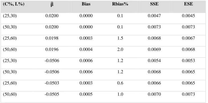
Table 4.1 shows the simulation result on the effect of the truncation time. According to
the table, the effect of the truncation time has been precisely estimated. The relative biases are
less than 2%. The estimated standard errors closely match the amount of variation in the
regres-sion coefficient estimates of the simulated sample. Larger variation is observed when censoring
rate or truncation rate is higher.
Regarding estimation of the distribution function of truncation time, we implemented two
methods: the Kaplan-Meier estimator for independently truncated sample given in Equation (2.4)
and the Kaplan-Meier estimator using the specially constructed risk set described in Section
3.3.1. For each method at time t, the average of the 1000 distribution function estimates was
ob-tained. Figure 4.1 shows the results for these two methods, together with the distribution of L.
In the figure, the dotted line is the true distribution function of L, the solid line is the estimation
result using the naïve Kaplan-Meier estimator, the dashed line is the estimation result using the
our new method with adjusted risk sets. From the figures we can see that the dashed line (new
method) highly agrees with the dotted line (true value), and the bias yielded in the naïve
Kaplan-Meier estimator is obvious.
We can conclude from Figure 4.1 that the regular left truncation version of Kaplan-Meier
estimator should be used with great caution on the required independence assumption. Such
test can be implemented to check the quasi-independence. For the relation assumed in Model
(3.2), the proposed estimator yields satisfactory result.
Table 4.1 Simulation result on the effect of truncation time for Model (3.2)
(C%, L%) 𝛃� Bias Rbias% SSE ESE
(25,30) 0.0200 0.0000 0.1 0.0047 0.0045 (50,30) 0.0200 0.0000 0.1 0.0073 0.0073 (25,60) 0.0198 0.0003 1.5 0.0068 0.0067 (50,60) 0.0196 0.0004 2.0 0.0069 0.0068 (25,30) -0.0506 0.0006 1.2 0.0054 0.0053 (50,30) -0.0506 0.0006 1.2 0.0068 0.0065 (25,60) -0.0503 0.0003 0.6 0.0066 0.0065 (50,60) -0.0505 0.0005 1.0 0.0070 0.0073
4.2 The Simulation Study for Model (3.3)
The simulation study in this section emphasizes on the scenario that predictors of T also
include one fixed covariate Z is associated with the failure time (Model (3.3)). The underlying
hazard function of the failure time T is given by,
𝜆(𝑡|𝐿,𝑍) =�𝜆𝜆�(𝑡)exp (𝛼𝑍), if 𝑡 <𝐿
�(𝑡) exp(𝛽𝐿+𝛼𝑍) , if 𝑡 > 𝐿
We still simulated the setting with positive and negative 𝛽 values, different truncation
rates, and different censoring rates. For the first set of simulated data, the covariate was
generat-ed from a standard normal distribution. The effect of the fixgenerat-ed covariate has been set to 1 and 0.5,
respectively. For the second set of simulated data, the covariate was generated from a Bernoulli
distribution with parameter value 0.5. The effect was set to 1. The simulation results for the
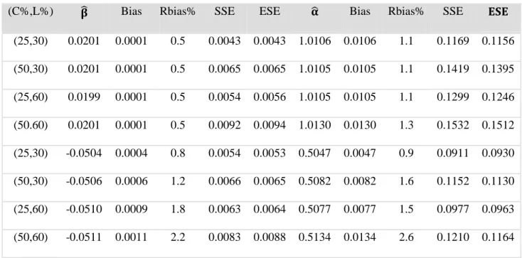
set-tings with continuous and discrete covariate are given in Table 4.2 and 4.3. In these two tables,
besides the result for the effect of truncation time, we similarly reported the estimation result for
the effect of covariate.
Regarding estimation of the distribution function of the truncation time, we implemented
three methods: the Kaplan-Meier estimator for independently truncated sample given in equation
(2.4), the Kaplan-Meier estimator given Z=0 in Section 3.3.1, and the K-M estimator given in
Section 3.3.2. Figure 4.2 describes estimation results for settings with continuous covariate. In
estima-tion (“left”), the long dashed line is the Kaplan-Meier estimator given in Secestima-tion 3.3.1 (“base”)
and the short dashed line is the Kaplan-Meier estimator given in Section 3.3.2 (“new”). We see
some improvements of the “base” method compared to naïve Kaplan-Meier estimator, but the
result from our new method is closest one to the true function. The simulation results for the
Table 4.2 Simulation result on regression coefficient estimation for Model (3.3) with a continuous covariate
(C%,L%) 𝛃� Bias Rbias% SSE ESE 𝛂� Bias Rbias% SSE 𝐄𝐒𝐄
(25,30) 0.0201 0.0001 0.5 0.0043 0.0043 1.0106 0.0106 1.1 0.1169 0.1156 (50,30) 0.0201 0.0001 0.5 0.0065 0.0065 1.0105 0.0105 1.1 0.1419 0.1395 (25,60) 0.0199 0.0001 0.5 0.0054 0.0056 1.0105 0.0105 1.1 0.1299 0.1246 (50.60) 0.0201 0.0001 0.5 0.0092 0.0094 1.0130 0.0130 1.3 0.1532 0.1512 (25,30) -0.0504 0.0004 0.8 0.0054 0.0053 0.5047 0.0047 0.9 0.0911 0.0930 (50,30) -0.0506 0.0006 1.2 0.0066 0.0065 0.5082 0.0082 1.6 0.1152 0.1130 (25,60) -0.0510 0.0009 1.8 0.0063 0.0064 0.5077 0.0077 1.5 0.0977 0.0963 (50,60) -0.0511 0.0011 2.2 0.0083 0.0088 0.5134 0.0134 2.6 0.1210 0.1164
Table 4.3 Simulation result on regression coefficient estimation for Model (3.3) with a discrete covariate
(C%,L%) 𝛃� Bias Rbias% SSE ESE 𝛂� Bias Rbias% SSE ESE
(25,30) 0.0199 0.0001 0.5 0.0046 0.0045 1.0119 0.0119 1.2 0.1891 0.1781 (50,30) 0.0198 0.0002 1.0 0.0073 0.0071 1.0080 0.0080 0.8 0.2266 0.2145 (25,60) 0.0197 0.0003 1.5 0.0065 0.0063 1.0089 0.0089 0.9 0.1989 0.1913 (50,60) 0.0198 0.0002 1.1 0.0104 0.0107 1.0062 0.0062 0.6 0.2312 0.2291 (25,30) -0.0508 0.0008 1.6 0.0055 0.0053 1.0083 0.0083 0.8 0.1802 0.1771 (50,30) -0.0511 0.0011 2.2 0.0069 0.0065 1.0062 0.0062 0.6 0.2144 0.2119 (25,60) -0.0505 0.0015 1.0 0.0063 0.0064 1.0099 0.0099 1.0 0.1951 0.1846 (50,60) -0.0510 0.0010 2.0 0.0085 0.0087 1.0042 0.0042 0.4 0.2228 0.2144
CHAPTER 5 EXAMPLES
5.1 Data Description
For the illustration purpose, we consider a transplant outcome data set from The Center
for International Blood and Marrow Transplant Research (CIBMTR). The CIBMTR is
com-prised of clinical and basic scientists who confidentially share data on their blood and bone
mar-row transplant patients with CIBMTR Data Collection Center located at the Medical College of
Wisconsin. The CIBMTR is a repository of information about results of transplants at more than
450 transplant centers worldwide.
Chemotherapy and Bone Marrow Transplant are two major treatments for leukemia
pa-tients. In our study, Chemotherapy data is from Pediatric Oncology Group and 540 children were
selected. BMT data is from International Bone Marrow Transplant Registry (IBMTR), and 376
children who received transplantation in second complete remission were selected. Due to
miss-ing values, 49 cases were excluded from the original data set. Thus, 527 cases of chemotherapy
and 340 cases of transplantation were used. For the BMT group, only the patients who received
transplants were observed, patients who died while waiting for transplantation were not included.
Thus, the BMT group is a truncated sample. The leukemia-free survival was the assessed in
Bar-rett’s study. To use this survival quantity, either leukemia relapse or death in remission should be
154 patients and the failure times were observed for 373 patients. The censored rate is about 29%.
For BMT group, 148 patients are censored and 192 patients experienced the failure events (death
or relapse). The censored rate is 44%.
Barrett el al. (1994) used the observational data to assess the treatment effect (BTM and
chemotherapy) and compare two competing risks on the leukemia-free survival. The following
factors are considered in Barrett’s data were sex, age, the leukocyte count at diagnosis (50,000
cells per cubic millimeter; 50.001-100,000 cells per cubic millimeter, >100,000 cells per cubic
millimeter), the T-cell phenotype (no; yes), duration of the first remission (≤ 18 months;
18.01-36 months; >18.01-36 months), and year of diagnosis (before 1984; after 1984).
Barrett et al. considered the matched pairs analysis and found a total of 255
matched-pairs between two treatment groups. In this study, our aim was to assess the effects of transplant
time and other risk factors on the failure time. We intended to employ different baseline hazard
rate functions for two treatment groups. Because there is no transplant time (truncation time) in
Chemotherapy group, we only focus on BMT group to estimate distribution of transplant time.
5.2 To Estimate the Treatment Effect and the Effects of Other Predictors
In Chapter 1, we have described the currently used Cox regression method to handle the
pooled sample of chemotherapy data and the BMT registry data. The current method assumes the
legiti-mate in randomized trial setting. In real applications, the chemotherapy sample and the BMT
sample come from different sources. Therefore, the common baseline hazard assumption is
high-ly suspicious.
We have suggested using Model (3.3) to allow different baseline hazard for two treatment
groups. The transplant time, with an assumed linear effect was included in the regressor. A
mod-el-building procedure was used to search for the significant risk factors with p-value 0.05 as the
threshold. Four factors, transplant time, age, duration of first remission, and T-cell
phenotype have been identified to be significant and hence included in the regressor. Since we
have a positive estimated effect for transplant time, the long waiting time leads to higher risks of
failure at future times. For age group, the estimated relative risks between children aged greater
than 10 and children aged at most 10 is 1.2185. The relative risk between the patients with the
duration of first remission in (18, 36) months and the patients with duration ≤18 months is
0.7913. The relative risk between the patients with duration of the first remission >36 months
and the patients with duration ≤18 months is 0.3594. The estimated relative risk between the
pa-tients with T-cell phenotypes and the papa-tients without T-cell phenotype is 1.4206.
Figure 5.1 shows the baseline cumulative hazard rates of chemotherapy group (solid line)
and BMT group (dashed line). Note that one patient received the transplant at month zero, so the
mea-ningful. The figure suggests different failure patterns for the chemotherapy group and the BMT
group.
Table 5.1 Regression coefficient estimates for the Cox model on the pooled sample
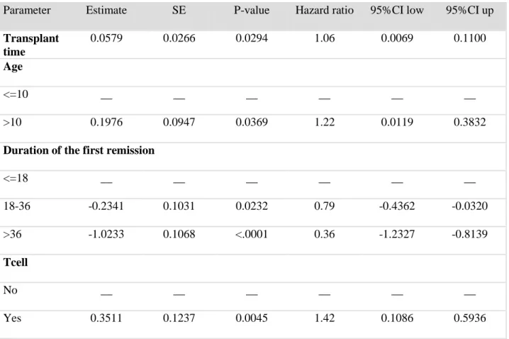
Parameter Estimate SE P-value Hazard ratio 95%CI low 95%CI up
Transplant time 0.0579 0.0266 0.0294 1.06 0.0069 0.1100 Age <=10 __ __ __ __ __ __ >10 0.1976 0.0947 0.0369 1.22 0.0119 0.3832
Duration of the first remission
<=18 __ __ __ __ __ __ 18-36 -0.2341 0.1031 0.0232 0.79 -0.4362 -0.0320 >36 -1.0233 0.1068 <.0001 0.36 -1.2327 -0.8139 Tcell No __ __ __ __ __ __ Yes 0.3511 0.1237 0.0045 1.42 0.1086 0.5936
Figure 5.1 Estimated cumulative hazard rates Chemotherapy group and BMT group
5.3 To Estimate the Distribution Function of the Transplant Time
In this section, we use the BMT sample only to estimate the distribution function of the
transplant time. The suggested Cox model was fitted for the BMT sample. Transplant time, age,
duration of first remission and T-cell phenotype were identified as significant factors and
in-cluded in the regressor. The estimated covariate effects were reported in Table 5.2. The effect of
waiting time remains the same. A long waiting time leads to a higher risk at future times.
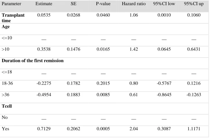
Table 5.2 Regression coefficient estimates for the Cox model on the BMT sample
Parameter Estimate SE P-value Hazard ratio 95%CI low 95%CI up
Transplant time 0.0535 0.0268 0.0460 1.06 0.0010 0.1060 Age <=10 __ __ __ __ __ __ >10 0.3538 0.1476 0.0165 1.42 0.0645 0.6431
Duration of the first remission
<=18 __ __ __ __ __ __ 18-36 -0.2275 0.1782 0.2015 0.80 -0.5767 0.1216 >36 -0.4954 0.1883 0.0085 0.61 -0.8645 -0.1263 Tcell No __ __ __ __ __ __ Yes 0.7129 0.2062 0.0005 2.04 0.3087 1.1171
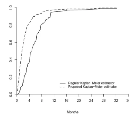
Using the estimation results from the Cox model and method described in section 3.3, we
ob-tained the estimates of the distribution of the transplant time. The estimation result is plotted in
Figure 5.2. Figure 5.2 also includes the result from the Kaplan-Meier method for an
Figure 5.2 Estimated distribution function of transplant time
Based on the BMT sample, we generated 5000 bootstrap samples with the same size. The
original sample contains 168 unique truncation times. A step function was constructed at these
168 time points. The 90% percentile confidence intervals and the 90% BCa bootstrap confidence
intervals were obtained and are shown in Figure 5.3 and 5.4, respectively. For this example,
Figure 5.3 90% percentiles confidence intervals for BMT bootstrap samples
CHAPTER 6 CONCLUSIONS
In this thesis, we proposed a new method for analyzing the left-truncated data with the
dependently truncation time and failure time. Truncation time L is considered as a covariate of
the failure time T and the distributions function of L were estimated in our simulation studies. A
real data example was also applied to the proposed method. Validation of our new model relies
on correct specification of the function k(L, β). In the simulation study, we assumed a linear ef-fect of the truncation time and the simulation result is satisfactory. The linear efef-fect of the
trun-cation time is the simplest form, in the future, we plan to conduct simulation study with more
complicated effect of truncation time. In practice, it may not easy to find an appropriate
func-tional form of L. In order to see if proposed method can handle the situation of misspecified
functional form of L, we can carry on some other simulation studies to test the robustness of our
new method. We have introduced Tsia’s Kandull’s tau tests to test the quasi-dependence between
failure time T and truncation time L in Section 2.3. However, Tsia’s tests were developed for
da-ta without ties. The BMT example analyzed in this thesis has a large number of ties among the
failure times and transplant times. This is the reason that we did not implementTsia’s test for the
BMT example. It is practically necessary to explore the solution to extend Tsia’s test to data with
REFERENCES
Andersen, P.K. 2005. Time-dependent covariate. Encyclopedia of Biostatistics, 2ed.ed. 8,
5467-5471. Wiley, New York.
Barrett, A.J., Horowitz, M.M., Pollock, B.H., Zhang, M.J., Bortin, M.M., Buchanan, G.R., Camitta, B.M., Ochs, J., Graham-Pole, J., Rowling, P.A., Rimm, A.A, Klein, J.P., Shuster, J.J., Sobocinski, K.A., Gale, R.P., 1994. HLA-identical Sibling Bone Marrow Transplants versus Chemotherapy for Children with Acute Lymphoblastic Leukemia in Second Re-mission. The New England Journal of Medicine331, 1253-1258.
Cox, D. R. 1972. Regression Models and Life Tables (with discussion). Journal of the Royal Statistical Society, Ser. B,34, 187-220.
Cox, D. R. 1975. Partial Likelihood. Biometrika 62, 269-276.
Efron, B., Tibshirani, R.J., 1993. An Introduction to the Bootstrap. Chapman and Hall/CRC
Keiding, N., Gill, R.D., 1990. Random truncation models and Markov processes. The Annals of Statistics 18, 582-602.
Klein, J.P., Moeschberger, M.L., 2003. Survival Analysis Techniques for Censored and Truncated Data. Springer-Verlag New York, Inc.
Klein, J.P., Zhang, M.J., 1996. Statistical Challenges in Comparing Chemotherapy and Bone-Marrow Transplantation as a Treatment for Leukemia. Life data: Models in relia-bility and Survival Analysis, (ed. N.P. et al.), 175-185.
Lai, T.L., Ying, Z., 1991. Estimating a distribution function with truncated and censored data. The Annals of Statistics19, 417-442.
samples applied to 3CR Quasars. Monthly Notices of the Royal Astronomical Society, Vol. 155, 95-118.
Nicoll, J.F., Johnson, D., Segal, I.E., Segal, W., 1980. Statistical invalidation on the Hubble Law. Proc. Natl. Acad. Sci. USA 77, 6275-6279.
Tsai, W.Y., 1990. Testing the assumption of independence of truncation time and failure time. Biometrika, 77, 169-177.
Wang, M.C., Jewell, N.P., Tsai, W.Y., 1986. Asymptotic properties of the product limit estimate under random truncation. The Annals of Statistics 14, 1597-1605.
Woodroofe, M., 1985. Estimating a distribution function with truncated data. The Annals of Statistics 13, 163-177.