Copyright
by
Hao Lyu
The Report committee for Hao Lyu
Certifies that this is the approved version of the following
report
Sarcasm Detection on Twitter
APPROVED BY
SUPERVISING COMMITTEE
Supervisor :
WALLACE, BYRON C
Sarcasm Detection on Twitter
by
Hao Lyu, B.M.S
Report
Presented to the Faculty of the Graduate School
of the University of Texas at Austin
in Partial Fulfillment
of the Requirements
for the Degree of
Master of Science in INFORMATION STUDIES
The University of Texas at Austin
May 2016
Sarcasm Detection on Twitter
by
Hao Lyu, M.S.INFO.STDS
The University of Texas at Austin, 2016
SUPERVISOR: Byron Wallace
Abstract: State-of-the-art approaches for sarcasm detection in social media combine lexical clues with contextual information surrounding the potentially sarcastic posting including author information. This article presents detailed methods for performing contextualizing sarcasm detection on Twitter, including data extraction, feature engineering and classification model settings. I reproduce the state-of-the-art results reported by Bamman and Smith (2015).
Contents
1 Introduction . . . 1
2 Data . . . 3
3 Data Extraction and Processing . . . 5
3.1 Data Crawling . . . 5 3.2 Data Processing . . . 6 4 Feature Engineering . . . 7 4.1 Tweet Features . . . 8 4.2 Author Features. . . 11 4.3 Audience Features . . . 13 4.4 Response Features . . . 13 5 Experimental Setting . . . 15
6 Result and Conclusion . . . 16
7 Acknowledgments . . . 18
1. Introduction
In recent years, the data generated from social media becomes more significant for companies and government. Data mining and analysis in blogs, postings and messages can foster great insights of social media users. These technologies can greatly improve the competitive advantage of companies, enhance the products and services and help decision making.
One obstacle for social media analysis is recognizing figurative language, such as sarcasm or irony. Sarcasm can be viewed as a special case of irony where the positive literal meaning is perceived as an indirect insult [3]. Sarcasm requires some shared knowledge between speaker and audience; it is a profoundly contextual phenomenon [1]. This master report is intended to reproduce the the sarcasm detection model and experiments reported in the recent work of Bamman and Smith, 2015.
Twitter is an online social networking service that enables users to send and read short 140-character messages called “tweets”. Many natural language processing tasks choose Twitter as the data source and conduct text mining on tweets, e.g., sentiment analysis, corpus annotation, linguistic pre-processing, information extraction and opinion mining. From a business and government point of view there is an increasing need to interpret and act upon information from large-volume social media streams, such as Twitter.
Sarcasm on Twitter is difficult to detect. Twitter users frequently use slang, emoticon, such as “: )” 1, hash tags and other jargon. Users are restricted by the 140 character limit of tweets which further complicates the matter. Traditional approaches rely on lexical clues of text. Work by Kreuk and Caucci indicate that sarcastic utterances often contain lexical indicators (such as interjections and intensifiers) and other linguistic markers (such as nonveridicality and hyperbole) that signal their irony.[4]
However, relying solely on intrinsic features of text is not always sufficient to recognize
sarcasm. Wallace et al.(2014) provided empirical evidence that humans can recognize sarcastic posts better when they are provided additional context surrounding the statements.[10] State-of-the-art methods for automatic sarcasm detection now rely on the contextualizing information surrounding the text. Sarcasm requires some shared knowledge between speaker and audience; it is a contextual phenomenon[1] [9].
In this report, I describe the re-implementation of a recent method for automatic sarcasm detection due to Bamman and Smith. This method combines lexical and contextual information to achieve robust classification performance. I will describe this method in detail and summarize my evaluation of my re-implementation.
In Section 2 I introduce the data I used in experiments. Then I present the data extraction and crawling from Twitter in Section 3. I discuss data processing and storage in Section 3. After preparing all the data needed, I present the detailed “features engineering” of this model in Section 4, which cost much time in my experiments. In Section 5, I will discuss the experimental setup and present the results. Section 6 concludes the report.
2. Data
Twitter provides rich text data and a wealth of contextualizing information. Millions of people tweet everyday. It is therefore a great source to conduct natural language processing experiments.
Figure 1 and Figure 2 show two illustrative examples of sarcastic tweets on Twitter
Figure 1: A sarcastic tweet. The speaker is clearly not welcoming allergy season back
Figure 2: A second sarcastic tweet. This speaker actually expresses frustration on Jiffylube
I chose tweets as my data source and conducted experiments to evaluate the model proposed by Bamman and Smith (2015). I use the same tweets in their experiments and the tweet list is provided by Bamman. This list contains In all 19534 tweets, around half sarcastic tweets, while the other half non-sarcastic tweets. However, tweets are diminishing with time goes, because users may quit Twitter, protect their accounts from viewing by public or delete tweets. After data crawling, I finally collected 17926 tweets.
The labels of tweets are inferred from self-declaration of sarcasm, e.g., a tweet is marked as sarcastic if it contains the hashtag #sarcasm or #sarcastic and non-sarcastic otherwise. This is an efficient way of collecting ‘labeled’ data, but may introduce some noise.
In addition, I also collected the historical(past) tweets of each author. The historical tweets in Bamman and Smith’s corpus are also disappearing, and the dataset I finally acquire
is thus not the exact same as the original dataset in Bamman and Smith’s experiment. This is in part because I do not have access to the Twitter “Gardenhose”2, so these data are scraped directly from the Twitter web pages. Twitter limits the volume of historical tweets written by one author that can be viewed by the public. Therefore I could only obtain around 850 tweets per user. Furthermore, the historical tweets of each author I collected were posted after they wrote the sarcastic tweet. Thus the historical tweets I collected may be different from those in Bamman and Smith’s dataset. However, it is reasonable to assume that the historical tweets I collect also qualitatively represent the same characteristics, preferences and past behaviors of the author as those collected by Bamman.
3. Data Extraction and Processing
3.1. Data Crawling
In this experiment, most tweets were collected using Python web crawlers and a few were collected from Twitter stream API. I define three different data crawling approaches:
• Static web crawler
• Dynamic web crawler
• Public Twitter stream API
The static web crawler scrapes static web pages and extracts text from the HTML markup. For example, I extracted these fields about the author from his/her Twitter web site: author’s name, the number of accounts he/she is following, the number of accounts following the author, the profile description, the time zone, and his/her duration on Twitter. The Python package “beautiful soup4” and “requests” support all the functions of static web crawling.
The dynamic web crawler focuses on the data sent from the Twitter server. When I interact with a website, e.g., scroll down the page to view more tweets from a user, JavaScript will detect my activity and send a request to the server. Then my browser will receive a response from the server containing all of the data I need, e.g., the tweets I would like to view, the followers’ names, or the historical tweets. On Twitter, their server will send back a JSON file back after my browser send the request. JSON is an open-standard format that uses human-readable text to transmit data objects consisting of attribute-value pairs. With the help of a JSON parser, I can extract needed information without manual effort. As long as the dynamic web crawler could simulate a browser, e.g., sending request and receiving response, I could parse the JSON data and convert them to meaningful data. This approach makes it feasible to collect historical tweets of users and who they are following.
The public Twitter Stream API makes it efficient to collect public tweets. Twitter provides an interface to developers using its API. Free accounts can extract 1 percent of all
public tweets, which comprises tweets in many languages. It is necessary to collect many public tweets randomly from Twitter when building a tweet dataset. The Twitter API works well in this scenario. However, free accounts will face a time limit rate problem when one tries to extract the historical tweets from one user. This problem will harm the speed of the crawler.
Anyone using these data crawling approaches will inevitably encounter the IP block. Twitter will block an IP of a crawler if it sends request to the server too frequently. This mechanism prevents the server from being attacked by DDOS. Two ways of overcoming the IP block are: 1. distribute the crawler across multiple machines, and 2. Set a random stop time after send k requests.
In my work, I deploy crawlers on five computing nodes in the computing clusters of TACC (Texas Advanced Computing Center). The crawlers will stop for a random number of seconds every time it sends 50 requests to the server, which assures no blocks happen.
3.2. Data Processing
The raw tweet and contextualizing data are difficult to use: tweets are written in various languages and length; and each author has a different timezone, which is hard to categorize. I normalize all tweets and process other data. I remove tweets not written in English, retweets, and tweets that contain fewer than three words. URLs and user mentions are replaced. The hashtag #sarcastic and #sarcasm in the Sarcastic tweets are also removed.
For the profile data, like timezone, I use Google geocoder package to map different locations to a similar area. Numbers in Twitter are displayed in string, e.g., “22K” or “2 Million”, and they need to be converted to numeric type.
All the data are stored into a database and the tweet IDs are used as the unique key for each tweet.
4. Feature Engineering
In this chapter, I introduce how to extract features for the machine learning model. Machine learning is a method used to devise complex models and algorithms that lend themselves to prediction. In machine learning and pattern recognition, a feature is an individual measurable property of a phenomenon being observed. The concept of “feature” is related to the explanatory variable used in statistical techniques such as linear regression. “Feature engineering” is the process of using domain knowledge of the data to create features
that make machine learning algorithms work.
It is an important procedure in machine learning and natural language processing to extract features from the data. This step is laborious but crucial for machine learning. Here I derive all of the features defined by Bamman and Smith (2015) in their original paper. The description of each feature is concise, but it is difficult to extract the features in practice. Below I explain each feature both in theory and practice.
For the sake of convenience and to avoid confusion, I will name the tweet I want to classify as sarcastic or not as the “target tweet”, the Twitter user who posted the tweet as “author”, the user who responded to, or was mentioned in the target tweet as “audience”,
and the tweet to which the target tweet responded as “original tweet”. The features used in this experiment are divided into four classes:
• Tweet Features
• Author Features
• Audience Features
4.1. Tweet Features
Tweet features represent the lexical and grammatical information of the target tweet. I can generate all the tweet features using only the tweet text, which reflect the literal meaning of the tweet. I explain all the features in this class above.
Bag of Words. The Bag of Words presentation is a simplifying representation used in natural language processing and information retrieval. In this model, a text (such as a sentence or a document) is represented as the bag (multiset) of its words, disregarding grammar and even word order but keeping multiplicity3. I extract binary indicators for the unigrams and bigrams in the target tweet. English stop words, e.g., ‘I’, ‘and’, ‘is’, are removed from the Bag Of Words. Python library Scikit-learn provides function to generate these features, represented by a huge binary sparse matrix.
Brown Cluster Unigrams and bigrams. Brown Clustering is a form of hierarchical clustering of words based on the contexts in which they occur. The intuition behind the model is ann-gram model, i.e. one in which we use indicators to encode words that occur[5]. Brown Clustering reduces the high dimensionality of the BoW model. I map each word in the 1000 non-overlapping clusters using the Brown Clusters of Owoputi et al., which group words used in similar context into the same cluster.[6] The 1000 clusters can be found on the website of TweetNLP4. By mapping unigrams and bigrams generated in the BoW to the Brown Clusters, I generate a smaller matrix, with 1000 columns.
Unlabeled dependency bigrams, lexicalized and Brown Clusters. Dependency is the notion that linguistic units, e.g., words, are connected to each other by directed links. Dependency parsing is a syntactic analysis that aims to understand the dependency relation in the sentence or document.
I use TweeboParser similar to Bamman and Smith’s experiment. This parser can also be found on the website of Carnegie Mellon University TweetNLP. After the TweeboParser
3https://en.wikipedia.org/wiki/Bag-of-words_model 4
parses one tweet, it generates pairs of words.
For a sentence like “the dog runs”, with unlabeled dependencies between “the −>dog” and “dog −>runs”, the binary lexicalized features would be:
“the −>dog”: 1 “dog−>runs”: 1
Then we can map these binary lexicalized features to the Brown Cluster. Suppose “the”
−>brown cluster #0, “dog” −> brown cluster #120, “runs” −>brown cluster #101, then binary brown cluster features would be:
“#0 −>#120”: 1 “#120 −> #101”: 1
Then we can run all tweets through the TweeboParser and generate these features.
Part of speech. Part of speech represents the category of words which have similar grammatical properties. Part of speech includes nouns, verbs, adjectives, adverbs, pronouns, prepositions, conjunctions, interjections, and sometimes numerals, articles or determiners.
I apply the part of speech tagger of Owoputi.[6] Carnegie Mellon University TweetNLP also provides a Java-based tokenizer and part-of-speech tagger for tweets. After training the tweets using their model, I calculate the density of all part of speech taggers including absolute count and ratio. These features can reflect the “lexical density” of the tweets.
Pronunciation features. Twitter users have specific writing styles, e.g., RT (Retweet), CHK (Check) and IIRC (If I recall correctly). To capture these language phenomena, I count the number of words that only have alphabetic characters but no vowels, and the words with more than three syllables. For this I use a regular expression.
Capitalization features. Capitalization is another language phenomena on Twitter. Users always show their emotions with capitalized words, e.g., “NO WAY” or “WTF”. I count the number of words that begin with caps and the number in all caps. The number of part of speech tags with at least initial caps are also extracted as a feature. This feature can also be identified using a regular expression.
Figure 3 shows a sarcastic tweet with capitalized words
Figure 3: A sarcastic tweet. “LOL” mean laugh out loud.
Tweet whole sentiment. Sentiment analysis is a significant part of understanding language. The apparent sentiment of a sarcastic tweet is usually different from its hidden meaning, i.e. critics might disparage a work by commending it sarcastically. I include several features that use of sentiment analysis. The first is the numeric value of the tweet determined by Stanford Sentiment Analysis[7]. This analyzer generates five values, representing “very negative”, “negative”, “neutral”, “positive” and “very positive”.
Another feature I include is the phrase-based sentiment ratio. Stanford Sentiment Analysis tries to determine the sentiment value of each non-terminal node in the parse tree of a sentence. I count the value of each node and calculate the fraction of different types of sentiment.
These features reflect the overall sentiment and sentiment distribution among the tweet itself. Stanford CoreNLP provides a Java based module to analyze sentences5. However it is slow because it uses neural network model. Therefore I use a distributed system to generate these features.
Tweet word sentiment. This feature is based on a word-level sentiment analysis. The sentiment strength of each word is estimated by the emotion scores of Thelwall[8]. The emotion effect of each word is mapped with the dictionaries of Warriner[11]. The maximum, minimum word sentiment/emotion score and the distance between the max and min are extracted.
5
SentiStrength is a Java based module that can estimate the strength of positive and negative sentiment in short texts. It reports 11 values from -5 to 5, which range from extremely negative to extremely positive. I generate all the word-level sentiment scores using it.
Warriner provides a list of 14,000 English lemmas that measure the emotion scores of words. By mapping the word in one tweet, I can refer all the effective scores. Then I build the features using the max value, min value and the distance between them.
Intensifier. Binary indicator for whether the tweet contains any intensifiers. Wikipedia provides 50 intensifiers to which I can map the word in the target tweet[12]. For instance, these intensifiers contain “amazingly”, “crazy”, “really”, “wicked” and “super”.
4.2. Author Features
Author features capture information about the author of the tweet, including historical data and the profile of the author. This class of features capture contextualizing information surrounding the target tweet. Knowing the author better can help the model determine whether he/she would likely post sarcastic tweets. One common idea is that the author may post negative tweets of an entity before, but the target tweet shows an inverse attitude or emotion to the entity. Then there may be a greater possibility that the target tweet is sarcasm.
The contextualizing features are as follows:
Author historical salient terms. Here TF-IDF score determines the feature. TF-IDF is short for“term frequency-inverse document frequency”. It is a statistic that is intended to reflect how important a word is to a document in a collection or corpus. The TF-IDF value increases proportionally to the number of times a word appears in the document, but is offset by the frequency of the word in the corpus, which helps to adjust for the fact that some words appear more frequently in general[13].
documents in the corpus,ft,d is the raw count of word t occurring in document d, tf(t, d) is
the term frequency score,idf(t, D) is the inverse document frequency score, andtf idf(t, d, D) is the TF-IDF score
tf(t, d) = 0.5 + 0.5∗ ft,d
max{ft0,d:t0 ∈d}
idf(t, D) =log N
|{d∈D:t∈d}|
tf idf(t, d, D) =tf(t, d)∗idf(t, D)
For each author, top 100 terms in their historical tweets with the highest TF-IDF scores are identified. After collecting all the top 100 terms, binary indicators are created for each author based on all the terms.
Author historical topics. Historical topic features are inferred under LDA with 100 topics over all tweets, where each document consists of up to 1000 words, similar to Bamman and Smith’s setting .[1] Each user’s topic proportions are collected as features.
LDA, short for Latent Dirichlet Allocation, is a generative statistical model that allows sets of observations to be explained by unobserved groups that explain why some parts of the data are similar[2].
I used the Python LDA package to train the model, setting the number of iterations to 8006. This feature estimates the topic preference of the author.
Profile information. This feature contains several fields from the user profile of the author, including number of accounts the author is following, number of accounts who follow the author, total number of tweets, author’s duration on Twitter, the average number of posts per day, author’s timezone, and whether or not the author is verified by Twitter.
Author historical sentiment. The distribution of sentiment in the historical tweets is modeled using word-level dictionaries, which are applied to tweet-level sentiment similar to the“tweet word sentiment feature”. I also use the Stanford Sentiment Analysis to estimate
6
the sentiment of each historical tweet and get the overall distribution of each author. These features represent the overall sentiment status of the author.
Profile unigrams. Twitter users always write a paragraph to describe himself or herself. The unigrams of this profile description are extracted as features.
4.3. Audience Features
Audience features encode information about the addressee of the tweet (the user to whom the predicted tweet is responding), including historical data, profile of the addressee and the communication between addressee, and the author of target tweet.
Audience historical topics, historical salient terms, profile information, pro-file unigrams. These features are similar to“Author historical topic”, “Author historical salient terms” and features in Author Features, but here I extract the feature from the historical tweets and profile information of the audience.
Author/Audience Interactional topics. This feature measures the similarity of historical topics of the audience and author. A topics matrix is generated by taking the element-wise product of the author and audience’s historical topic distribution. Similar topics will result in larger value in the distribution.
Historical communication between author and audience. This feature measures the degree of familiarity of author and audience. I extract the rank of the audience in author’s @-mention list, and also whether or not there have been mutual @-mention messages in the historical tweets of both, the number of messages sent from the author to the audience are extracted into this feature. Using a regular expression, I match these rules and search in the historical tweets of author and audience.
4.4. Response Features
Response Features consider the interaction between the target tweet and the tweet that it is responding to. The original tweet is usually talking about a similar subject as the target
tweet.
Pairwise Brown features between the original message and the response. This feature captures the interaction between the target tweet and the original tweet. I model the ‘Brown cluster unigrams and bigrams’ of the original tweet as described earlier. I also introduce binary indicators of pairwise Brown features between all terms in the two tweets.
Unigram features of original message. This feature encodes the ungirams of the original tweet using Bag of Words. Binary indicators of all unigrams are extracted as features.
5. Experimental Setting
The experimental methodology is similar to that in Bamman and Smith’s way.[1] Some tweets in my dataset are missing fields. I remove these tweets. My final tweets dataset contains 11,457 tweets, 6550 are sarcastic tweets and 4907 are non-sarcastic.
For a classification model, I use binary Logistic Regression to predict whether a tweet is sarcastic or not. L2 regularization is applied to prevent over-fitting. In the fields of machine learning, we always introduce an additional regularization term to the general loss function. This method attempts to introduce a penalty for over-fitting and improve generalization. Regularization can be used to learn simpler models, induce models to be sparse, and introduce group structure into the learning problem.
To assess performance, I performed tenfold cross-validation. The data are split into 10 folds and I tune the L2 parameter with 1/10 data, train the model with 8/10 data, and evaluate the model with held-out 1/10 data. This process is repeated across the 10 folds.
All the features mentioned in the feature engineering are extracted from the data. Nu-merical features scaled between 0 and 1. Categorical features are normalized by binarization, e.g., each categorical feature with m possible values intom binary features, with only one active.
6. Result and Conclusion
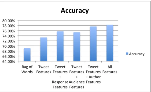
To compare the performance of different features, I consider 6 combinations and use the Bag of Words model as the baseline. Here are the accuracy results of different combinations, also shown in Figure 4.
• Bag of Words (baseline): 69.1%
• Tweet Features: 73.3%
• Tweet Features + Response Features: 75.7%
• Tweet Features + Audience Features: 75.3%
• Tweet Features + Author Features: 77.6%
• Tweet Features + Author Features + Audience Features + Response Features: 78.3%
Combining all features can produce the best accuracy 78.3%. Tweet features can be viewed as the lexical and grammatical clues in tweets. Other feature sets can be understood as surrounding contextualizing information. Author features improve the greatest accuracy over the tweet only. This means the historical tweets and profile information can be viewed as the best contextualizing indicators of sarcasm.
However, collecting historical tweets data is very expensive in both human and compute time. It is not practical to use all historical data of one author to predict whether or not his/her tweet is sarcastic. I suggest using less contextualizing information of the author, especially the data that can be collected easily and fast. For instance, the profile information of the author and the response features are relatively effective and costs less. The features extracted from the historical tweets, especially the salient terms and topic distributions, improve the model enormously. I suggest the model only extract the historical tweets around the target tweet. From intuition, these surrounding tweets posted in closer time would probably emphasize the similar object more often. Meanwhile, random sampling from the historical tweet can also both generate the topic distribution and reduce cost.
7. Acknowledgments
I thank my project supervisor Professor Byron Wallace for his help and encouragement. I’m grateful to my program adviser Professor James Howison for his assignments that kept me pushing. I also thank my collaborator Silvio Moreira and his suggestions to make this work better. Thank you, UT Austin School of Information, for my Master ’seducation. I’m proud to be a longhorn!
8. References
[1] David Bamman and Noah A. Smith. Contextualized sarcasm detection on twitter.
In Proceedings of the 9th International Conference on Web and Social Media, pages 574–577, April 2015.
[2] Andrew Y. Ng Blei, David M. and Michael I. Jordan. Latent dirichlet allocation. the Journal of machine Learning research, 3:993–1022, 2003.
[3] S. Dews and E. Winner. Muting the meaning A social function of Irony. Metaphor and Symbol, 10(1) edition, 1995.
[4] R.J. Kreuz and G.M. Caucci. Lexical influences on the perception of sarcasm. in proceedings of the workshop on computational approaches to figurative language.
Association for Computational Linguistics, pages 1–4, April 2007.
[5] Percy. Liang. Semi-supervised learning for natural language. Diss. Massachusetts Institute of Technology, 2005.
[6] Olutobi Owoputi, Brendan O’Connor, Chris Dyer, Kevin Gimpel, Nathan Schneider, and Noah A. Smith. Improved part-of-speech tagging for online conversational text with word clusters. Association for Computational Linguistics, 2013.
[7] Richard Socher, Alex Perelygin, Jean Y. Wu, Jason Chuang, Christopher D. Manning, Andrew Y. Ng, and Christopher Potts. Recursive deep models for semantic composi-tionality over a sentiment treebank. Proceedings of the conference on empirical methods in natural language processing (EMNLP)., 1631, 2013.
[8] Thelwall, M and Buckley K, Paltoglou G, Cai D, Kappas A. Sentiment strength detection in short informal text. Journal of the American Society for Information Science and Technology, 61.12:2544–2558, 2010.
[9] Byron C. Wallace. Sparse, contextually informed models for irony detection: Exploiting user communities, entities and sentiment. In ACL, 2015.
[10] Byron C. Wallace, Laura Kertz Do Kook Choe, and Eugene Charniak. Humans require context to infer ironic intent (so computers probably do, too). In ACL, pages 512–516, April 2014.
[11] Victor Kuperman Warriner, Amy Beth and Marc Brysbaert. Norms of valence, arousal, and dominance for 13,915 english lemmas. Behavior research methods, 45.4:1191–1207, 2013.
[12] Wikipedia. ‘intensifier’ — Wikipedia, the free encyclopedia., 2016. [Online; accessed 03-May-2016].
[13] Wikipedia. ‘tf-idf’ — Wikipedia, the free encyclopedia., 2016. [Online; accessed 03-May-2016].