The Control, Manipulation and Detection
of Surface Plasmons and Cold Atoms
Sanele Goodenough Dlamini
School of Chemistry and Physics
University of KwaZulu-Natal
A thesis submitted in fulfillment of the requirements for the degree of
Doctor of Philosophy
Abstract
Cold atoms and surface plasmons are now widely recognised as having a vast potential as sources for future quantum information technologies, including in quantum sim-ulations, quantum computing and quantum-enhanced metrology. In the first part of this Thesis an experimental investigation of the decoherence of single surface plasmon polaritons in plasmonic waveguides is carried out. In the study, a Mach-Zehnder con-figuration previously considered for measuring decoherence in atomic, electronic and photonic systems, is used. By placing waveguides of different lengths in one arm mea-surements of the amplitude damping time, pure phase damping time and total phase damping time were achieved. Decoherence was found to be mainly due to ampli-tude damping and thus losses arising from inelastic electron and photon scattering play the most important role in the decoherence of plasmonic waveguides in the quantum regime. However, pure phase damping is not completely negligible. In the second part of the Thesis the properties of light in the fundamental mode of a subwavelength-diameter plasmonic nanowire are also investigated. One of the applications of the light is the trapping of atoms by the optical force of the evanescent field and the subsequent guiding of the emitted light from the atoms. The quantum correlation functions of the emitted light from different numbers of atoms into the wave guided mode of the nanowire are investigated analytically. It is found that the nanowire provides an ef-ficient method of generating quantum states of light - it gives a faster time scale for the dynamics and improved coupling efficiency compared to an equivalent dielectric nanofiber. The results of this Thesis will be useful for the design of plasmonic wave-guide systems for carrying out phase-sensitive quantum applications, such as quantum sensing, and for the generation of novel quantum states of light for quantum comput-ing and quantum communication. The probcomput-ing techniques developed for the plasmonic waveguides may also be applied to other types of plasmonic nanostructures, such as those used as nanoantennas, as unit cells in metamaterials and as nanotraps for cold atoms.
Preface
The work reported in this dissertation was carried out in the School of Chemistry and Physics, University of KwaZulu-Natal, under the supervision of Prof. Francesco Petruccione, Prof. Mark Tame and Prof. S´ıle Nic Chormaic.
As the candidate’s supervisors we have approved this dissertation for submission.
Prof. F. Petruccione Date
Prof. M.S. Tame Date
Prof. S. Nic Chormaic Date
6 December 2017 6 December 2017
Declaration
I, Sanele Goodenough Dlamini declare that
1. The research reported in this thesis, except where otherwise indicated, is my orig-inal research.
2. This thesis has not been submitted for any degree or examination at any other university.
3. This thesis does not contain other persons’ data, pictures, graphs or other infor-mation, unless specifically acknowledged as being sourced from other persons.
(a) This thesis does not contain other persons’ writing, unless specifically ac-knowledged as being sourced from other researchers. Where other written sources have been quoted, then:
(b) Their words have been re-written but the general information attributed to them has been referenced; Where their exact words have been used, their writing has been placed inside quotation marks, and referenced.
4. This thesis does not contain text, graphics or tables copied and pasted from the Internet, unless specifically acknowledged, and the source being detailed in the thesis and in the References sections.
Publications
1. S. Dlamini, J. Francis, X. Zhang, S. Nic Chormaic, S¸. K. ¨Ozdemir, F. Petruccione and M. Tame, Probing decoherence in plasmonic waveguides in the quantum
regime, submitted to Physical Review Applied, preprint available at https://arxiv.org/abs/1705.10344 (2017)
2. Y. Ismail, S. Dlamini, M. Morrissey, R. Tridib, C. Karlsson, S. Nic Chormaic and F. Petruccione, Magneto Optical trapping of85Rb- Cold atoms, submitted for publication in the Proceedings of the 62nd annual conference of The South African Institute of Physics (2017).
3. S. G. Dlamini, F. Petruccione, S. Nic Chormaic and M. S. Tame, Quantum emis-sion of cold atoms into plasmonic nanowire waveguides, in preparation (2017).
Acknowledgements
I would like to thank Prof. Francesco Petruccione, Prof. Mark Tame and Prof. S´ıle Nic Chormaic. I would also like to thank Dr. Fam Le Kien on the discussion we had on nanofibers and nanowires.
This research was supported by the South African Research Chair Initiative of the De-partment of Science and Technology and the National Research Foundation.
Contents
1 Introduction 13
1.1 Background . . . 13
1.2 Aim and Approach . . . 16
1.3 Outline . . . 16
2 Basic Tools and Techniques 18 2.1 Surface Plasmon Polaritons . . . 18
2.2 Quantization of Photons and Plasmons . . . 21
2.2.1 Quantization of the Free-Space Electromagnetic Field . . . 21
2.2.2 Quantization of Surface Plasmons . . . 24
2.3 Single-Photon Source . . . 24
2.3.1 Introduction . . . 24
2.3.2 Theory . . . 25
2.3.3 Experimental Setup . . . 27
2.3.4 Results . . . 28
3 Probing Decoherence in Plasmonic Waveguides in the Quantum Regime 29 3.1 Introduction . . . 29
3.2 Experimental setup . . . 31
3.3 Results . . . 32
3.4 Discussion . . . 42
4 Atomic Emission into Nanophotonic Waveguides 43 4.1 Field Expressions in an Optical Fiber . . . 43
4.2 Field Expressions in a Nanowire . . . 47
4.3 Photon and SPP Correlations Emitted by Atoms into Nanophotonic Waveguides . . 51
4.3.2 Atomic Gas . . . 60
List of Figures
1.1 Experiments with metalic nanostructures. . . 15 2.1 Charges and electromagnetic field lines of a SPP propagating on a metal (1 and
z<0) and dielectric (2andz>0) interface along the x-direction. . . 19
2.2 Experimental setup for single photon source . . . 27 3.1 Experimental setup for probing the decoherence of single surface plasmon
polari-tons (SPPs). . . 30 3.2 Decoherence in the classical and quantum regime. . . 34 3.3 Dispersion curve for light in a stripe waveguide. . . 35 3.4 Intensity dependence of the output signal from the MZI in the classical and quantum
regimes for different waveguide length as the phaseφis modified. . . 39 4.1 Intensities |Ez|2, |Er|2, and |Eϕ|2 of the cylindrical-coordinate components of the
field in theHE11mode with circular polarization. . . 45
4.2 Azimuthal profiles of the intensities|Ex|2,|Ey|2, and|Ez|2of the Cartesian-coordinate
components of the electric field in theHE11mode with circular polarization. . . 46
4.3 Cross-section profiles of the intensities|Ex|2,|Ey|2, and|Ez|2of the Cartesian-coordinate
components of the electric field in theHE11mode with circular polarization. . . 47
4.4 Nanofiber electric field density plots. (a) Magnitude of the total electric field|E| =
q
|Er|2+|Ez|2+|Eϕ|2. (b) Magnitude of the transverse electric field|E|= q
|Er|2+|Eϕ|2.
(c) Magnitude of the longitudinal electric field|E|=|Ez|. . . 48
4.5 Field plot of the electric field component in theHE11mode for circular polarization.
The following parameters have been used: n1 = 1.45, n2 = 1, a = 200 nm and λ=852 nm.(a) The field inside the fiber. (b) The field outside the fiber. . . 49 4.6 Model of geometry in a nanowire. . . 49
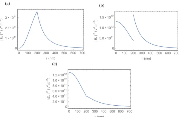
4.7 Intensities|Ez|2and|Er|2of the cylindrical-coordinate components of the field in the
HE11mode of a nanowire. The wire has radiusa= 200 nm with2 = −28.5+2i
and1=1. The free space wavelength isλ=852 nm. . . 50
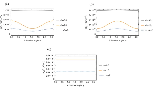
4.8 Azimuthal profiles of the intensities|Ex|2,|Ey|2, and|Ez|2of the Cartesian-coordinate
components of the electric field in a fundamental mode nanowire. . . 50 4.9 Cross-section profiles of the intensities|Ex|2,|Ey|2, and|Ez|2of the Cartesian-coordinate
components of the electric field of theHE11mode in a nanowire. . . 51
4.10 Nanowire electric field density plot. (a) Magnitude of the total electric field|E| =
p
|Er|2+|Ez|2. (b) Magnitude of the transverse electric field|E|= p
|Er|2. (c)
Mag-nitude of the longitudinal electric field|E|=|Ez|. . . 52
4.11 Field plot of the electric field component in theHE11mode of silver nanowire. The
following parameters have been used: 2 = −28.5+2i,1 = 1,a = 200 nm and
λ=852 nm. (a) The field inside the wire. (b) The field outside the wire. . . 52 4.12 Model of geometry in a nanophotonic waveguide. . . 53 4.13 Experimental setup for measuring first-order and second-order correlation function. 56 4.14 Normalized first-orderg(1)N (τ) and second-orderg(2)N (τ) correlation functions. . . 57 4.15 Normalized first-orderg(1)N (τ) and second-orderg(2)N (τ) correlation functions for N
atoms in an array near a nanofiber of radiusa=25 nm. . . 57 4.16 Normalized first-orderg(1)N (τ) and second-orderg(2)N (τ) correlation functions for N
atoms in an array near a nanowire of radiusa=200 nm. . . 58 4.17 Normalized first-orderg(1)N (τ) and second-orderg(2)N (τ) correlation functions for N
atoms in an array near a nanowire of radiusa=25 nm. . . 58 4.18 Normalized first-orderg(1)N (τ) and second-orderg(2)N (τ) correlation functions for atomic
gas around a fiber of radiusa=200 nm. . . 61 4.19 Normalized first-orderg(1)N (τ) and second-orderg(2)N (τ) correlation functions for atomic
gas around a fiber of radiusa=25 nm. . . 62 4.20 Normalized first-orderg(1)N (τ) and second-orderg(2)N (τ) correlation functions for atomic
gas around a nanowire of radiusa=200 nm. . . 62 4.21 Normalized first-orderg(1)N (τ) and second-orderg(2)N (τ) correlation functions for atomic
List of Tables
2.1 Count rate results at zero time delay. . . 28 3.1 Summary of results from probing decoherence in plasmonic waveguides. . . 41
List of Abbreviations
SPP Surface plasmon polariton
SPDC Spontaneous parametric down-conversion
SPAD Single-photon silicon avalanche photodiode detector BBO Beta Barium Borate
SM Single-mode fiber MM Multimode fiber
PM Polarization maintaining fiber MZI Mach-Zehnder interferometer AD Amplitude damping PD Phase damping BS Beamsplitter PBS Polarising beamsplitter HWP Half wave-plate QWP Quarter-wave plate LP Linear polarizer
Chapter 1
Introduction
1.1
Background
Plasmonic systems involve electromagnetic excitations of light coupled to electron charge den-sity oscillations on the surface of metals [1]1. These hybrid excitations of light and matter are known as surface plasmon polaritons (SPPs) and the electromagnetic field is highly confined [2, 3]. This confinement has opened up many applications for controlling light at the nanoscale, including nanoantennas for sending and receiving light signals [4], the enhancement of photovoltaics for solar cell technology [5], and many more [6]. The hybrid nature of SPPs has also raised the interesting prospect of integrating photonics and electronics in the same platform [7]. Most recently, studies have investigated plasmonics in the quantum regime [8], with single-photon sources [9–12] and single-photon switches [13–15] being proposed and experimentally realized. These nanophotonic devices are important for emerging quantum technologies, such as photonic-based quantum com-puters [16, 17] and quantum communication networks [18]. Recent work has also demonstrated several key quantum applications, including quantum sensing [19–21], quantum spectroscopy [24], quantum logic gates [25], entanglement generation [26] and distillation [27], and quantum random number generation [28]. What is surprising is that all of these applications can be realized even in the presence of loss, which is ever present in plasmonic systems as they are scaled down to confine light to smaller scales.
In the classical regime, loss has been studied extensively, both in plasmonic nanostructures and waveguides [1]. At the microscopic level, loss is mainly due to the electron dynamics in the metal,
which are governed by electron-electron scattering events, and electrons scattering with other charge carriers, phonons, defects and impurities [29]. In the quantum regime, loss – commonly referred to as amplitude damping [30] – has recently been studied in terms of its impact on the quantum statis-tics of single SPPs in waveguides [31, 32]. However, in addition to loss of amplitude, an important factor that needs to be taken into account is loss of coherence, both spatial and temporal [33]. In the classical regime, there have been many works that have investigated loss of coherence in plas-monic nanostructures and waveguides, both spatially [34–37] and temporally [38–42, 68]. At the microscopic level, pure loss of coherence is due to elastic electron scattering processes that do not lead to the loss of energy from the plasmon oscillation [38, 69]. In the quantum regime, loss of co-herence – commonly referred to as phase damping [30] – has not yet been studied for single SPPs. While results in the classical regime suggest that phase damping does not have a significant impact on the plasmon dynamics in nanostructures [38] and in waveguides of short length [68], it is not yet known how low-level excitations of light are affected, nor what role it may play in the plasmon dynamics in longer waveguides. Given the increasing number of applications already demonstrated for plasmonics in the quantum regime it is important to understand the relative impact of amplitude damping, which also causes loss of coherence, and phase damping, so that phase-sensitive quantum applications may be properly developed. This is the first of the two main topics investigated in this Thesis.
With the rapid developments in the fields of quantum computation and quantum information sci-ence, there has been growing interest in investigating new physical mechanisms that allow coherent coupling between individual quantum systems and photon fields. Coupling between optical emitters and light fields is one of the outstanding goals in quantum technology [43]. This may lead to many possible applications, for example the generation of single photons on demand [44], the control of the emission rate of quantum emitters [45], and the construction of single-photon transistors [13] that would also facilitate the scalability of quantum computers. A stronger concentration of opti-cal fields is possible with surface plasmons compared to conventional dielectric methods [46]. In this setting, strong coupling is being pursued by combining emitters with nanophotonic waveg-uides [47–49]. Akimovet al.have demonstrated a 2.5 fold enhancement in the emission of a single quantum dot into the SPP mode of a silver nanowire and observed that the light scattered out of the end of the nanowire is anti-bunched [9], as depicted in Fig 1.1 (a) and (b). The unique properties of plasmons on this kind of metallic nanostructure have produced various effects such as
single-(a) (b) (a) (b) (c) (e) (c) (e) (d) (d)
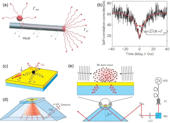
Figure 1.1: Experiments with metalic nanostructures. a) Quantum dot emission into SPP modes of a silver nanowire. The quantum dot decays into free space modes and SPP modes with ratesΓradand
Γplrespectively. b) Self-correlation coincidences of the scattered light from SPP modes [9]. c) An
atom near a metal surface emits photons withγrad into free space andγspinto SPPs guided modes
on the metal surface. d) SPPs on a thin metal film couple to the far field in the dielectric substrate by leakage radiation. The emitted light field is p-polarized. A detector collects photons under the solid angle∆Ω. e)Rbcold atoms near a gold film. Emitted photons are collected by an optical fiber coupler (FC) and detected with single-photon detectors [89].
molecule detection with surface-enhanced Raman scattering, and enhanced transmission through subwavelength apertures. There is an increasing interest in these systems for applications such as biosensing [50, 51] and subwavelength imaging [37].
Furthermore, proposals for trapping not just one emitter, but many in the form of ultracold atoms placed close to plasmonic structures have received much attention recently [52–54]. The proposals are based on the concept of dipole traps that are generated above plasmonic nanostructures, similar to the optical trapping of nano-objects in plasmonically patterned light fields [55]. Atoms have the advantage of being identical quantum emitters and have very narrow optical transitions with typical widths in the megaHertz range. Using quantum optics techniques, clouds of atoms can be cooled
to quantum degeneracy at temperatures of the order of nanoKelvins [56]. The atoms are trapped with ultrahigh precision in magnetic microtraps in optical dipole traps where they suffer very low intrinsic decoherence [57–59]. Stehleet al.have demonstrated cooperative coupling of ultracold atoms with surface plasmons propagating on a plane gold surface [89] , as depicted in Fig. 1.1 (c), (d) and (e). Plasmonic traps improve the control over the motion of atoms in the subwavelength regime even further. Atoms that are positioned very close to plasmonic structures couple with high efficiency to surface plasmon modes, which could be used for single-photon applications and for enabling long-range interactions between atoms [52, 54]. Strong coupling is also acheived by com-bining cold atoms with nanophotonic waveguides [47–49]. Kumar et al. have demonstrated the propagation of higher order modes in an optical nanofiber integrated into a magneto optical trap for neutral atoms [60]. In the dielectric waveguides it has been shown that a significant fraction of emission from a single atom can be coupled into a nanofiber [61]. The quantum correlations of photons emitted into a nanofiber have also been measured [62]. It is still unclear how metallic waveguides supporting surface plasmons perform in this setting. This is the second of the two main topics investigated in this Thesis.
1.2
Aim and Approach
The goal of this study is to use the techniques of quantum optics to investigate the fundamental quantum mechanics of surface plasmons, to probe decoherence of plasmonic waveguides in the quantum regime and to investigate the quantum properties of light generated from atomic decay into the fundamental mode of a subwavelength-diameter plasmonic nanowire.
1.3
Outline
An experimental investigation of the decoherence of single surface plasmon polaritons in plasmonic waveguides is carried out. The properties of light in the fundamental mode of a subwavelength-diameter plasmonic nanowire are investigated. The aim of this thesis is to describe this work, in the appropriate theoretical context and describing the methods of the experiment in detail for other researchers to be able to reproduce and extend them. The chapters are organized as follows:
• In Chapter 2 the basic tools and techniques required to understand and evaluate the remain-der of the thesis are described. The simplest classical description of the surface plasmon is
given, which models the metal as a gas of free, independent electrons that move under the influence of an applied field. Then the procedure for quantizing electromagnetic waves is described and it is summarized how the same procedure can be applied to surface plasmons, drawing on the analogy between the photon and the plasmon. Lastly a description is given about the main ideas behind spontaneous parametric down-conversion (SPDC), the nonlinear optical phenomenon used to generate pairs of single photons used in the experiment on the decoherence of SPPs.
• In Chapter 3 the decoherence of SPPs in plasmonic waveguides in the classical and quantum regimes is investigated. Both amplitude and phase damping effects of SPPs are measured. For classical SPPs and single SPPs, it was discovered that amplitude damping is the main source of amplitude and phase decay. The results will be useful in the design of phase-sensitive quantum plasmonic applications, such as quantum sensing and allow appropriate quantum states to be chosen for a given task to be achieved
• In Chapter 4 the atomic emission into nanophotonic waveguides is then presented. A descrip-tion of the properties of light in the fundamental mode of a subwavelength-diameter dielectric fiber is given. This is followed by the description of the properties of light in the fundamental mode of a subwavelength-diameter silver nanowire. The correlations of the photons emitted by fluorescence from atoms and an atomic cloud of atoms into guided modes of a nanofiber are investigated, as well as the correlations between SPPs emitted by fluorescence into guided modes of a silver nanowire.
Chapter 2
Basic Tools and Techniques
This chapter presents the theory that is required throughout this Thesis. It begins with a discussion on surface plasmons, a totally classical result based on Maxwell’s equations. In quantum theory, in contrast, excitations of surface plasma waves come in discrete energy steps. Like photons, singular surface plasmons are indivisible and must be added to or subtracted from surface plasma waves in number products. In accordance with this, the quantization of the free-space electromagnetic field and that of surface plasmons is discussed. The chapter ends of with the description of a single-photon source.
2.1
Surface Plasmon Polaritons
So as to investigate the properties of SPPs, we begin from Maxwell’s equations [64, 65]:
∇ ·D=ρ, (2.1a) ∇ ·B=0, (2.1b) ∇ ×E=−∂B ∂t, (2.1c) ∇ ×H=j+∂D ∂t, (2.1d)
whereDis the dielectric displacement,Eis the electric field,His the magnetic field, and Bis the magnetic flux density. Without the external charge and current densities (∇ ·D = 0 andj = 0) Eqs. (2.1c) and (2.1d) can be combined to form the wave equation
∇2E− c2
∂2E
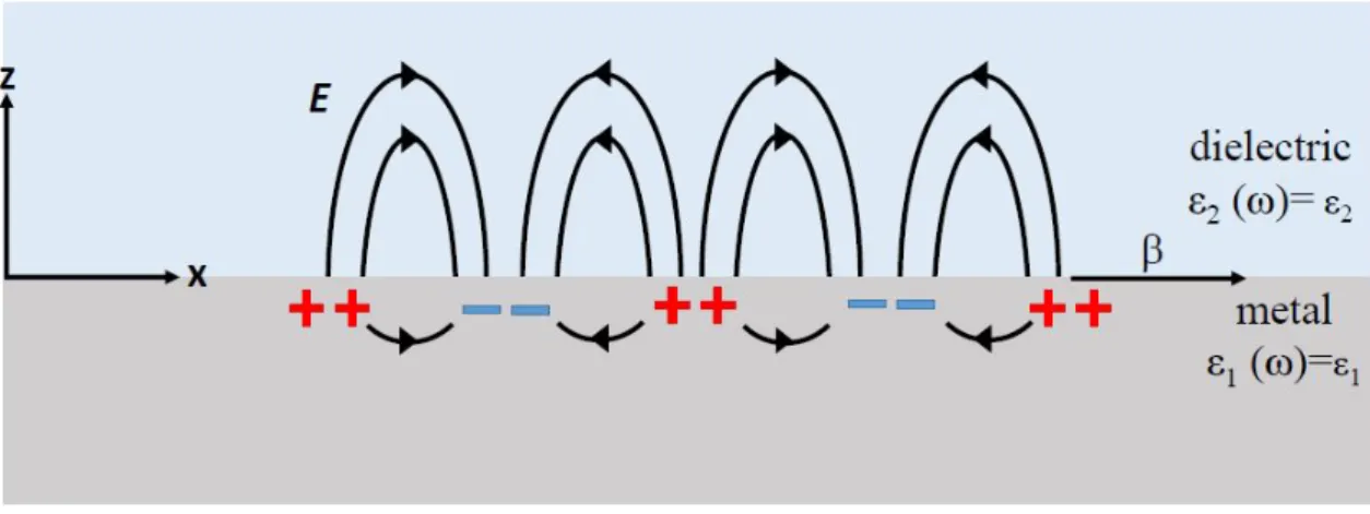
Figure 2.1: Charges and electromagnetic field lines of a SPP propagating on a metal (1andz <0)
and dielectric (2andz>0) interface along thex-direction.
where is the dielectric function of the material the electric field is in. To start with, assume a harmonic time dependenceE(r,t) = E(r)eiωt of the electric field and substitute it into Eq. (2.2) to give
∇2E+k20E=0, (2.3) andk0 = ωc is the vacuum propagation constant. Consider surface plasma waves propagating in
the x-direction. Since the geometry is thought to be infinitely long in the y-direction, the elec-tromagnetic field has no spatial dependence along the y-direction, as shown in Fig. 2.1. Now
E(x,y,z) = E(z)eiβx where β is the propagation constant. Substituting this into Eq. (2.3) yields the following form of the wave equation
∂2E(z)
∂z2 +(k 2
0−β2)E=0. (2.4)
In the same way the equation for the magnetic fieldHis obtained ∂2H(z)
∂z2 +(k 2 0−β
2)H=0. (2.5)
For time-harmonic dependence (∂∂t =−iω) and propagation along thex-direction (∂∂x =iβ) with no spatial variation along they-direction (∂∂y =0) Eq. (2.1c) and (2.1d) for different field components ofHandEare simplified as follows:
∂Ey
∂z =−iωµ0Hx, (2.6a)
∂Ex
iβEy =iωµ0Hz, (2.6c) ∂Hy ∂z =iω0Ex, (2.6d) ∂Hx ∂z −iβHz=−iω0Ey, (2.6e) iβHy=−iω0Ez. (2.6f)
The guided electromagnetic modes have two solution sets, one for transverse magnetic (TM) modes or transverse electric (TE) modes. For TM modes where only Ex, Ez and Hy are nonzero the
equations reduce to Ex= −i ω0 ∂Hy ∂z , (2.7) Ez= −β ω0 Hy, (2.8)
and by sustituting Eqs. (2.7) and (2.8) into the wave equation (2.4) yields the TM modes wave equation which is given by
∂2H y ∂z2 +(k 2 0−β 2)H y=0. (2.9)
From the solution of Eq. (2.9) and Eqs. (2.7) and (2.8) the field components can be found for
z>0 Hy(z)=A2eiβxe−k2z, (2.10a) Ex(z)=iA2 1 ω02 k2eiβxe−k2z, (2.10b) Ez(z)=−A1 β ω02 eiβxe−k2z, (2.10c) and forz<0 Hy(z)= A1eiβxek1z, (2.11a) Ex(z)=−iA1 1 ω01 k1eiβxek1z, (2.11b) Ez(z)=−A1 β ω01 eiβxek1z, (2.11c) where k2i =β2−k02i (i=1,2) (2.12)
is the component of the wave vector perpendicular to the interface in the two regions andkz =
(−1)iki. The continuity ofHyandEzat the interface means that
A1=A2=⇒ k2 k1 =−
2
1
By substituting this relation into Eq. (2.12) the dispersion relation of SPPs is given by β=k0 r 12 1+2 . (2.14)
This equation is valid for both real and complex1. Carrying out a similar procedure for the TE
modes leads to the conclusion that no TE surface modes can exist due to the geometry of the sys-tem.
2.2
Quantization of Photons and Plasmons
2.2.1 Quantization of the Free-Space Electromagnetic Field
The electric and magnetic fields can both be written in terms of the vector potentialA(r,t) using the following relationsE(r,t)=−∂A∂(rt,t) andB(r,t)=∇ ×A(r,t). In the Coulomb gauge,∇·A(r,t)=0, the vector potential can be thought of as the electromagnetic field, i.e. a field that represents both the electric and magnetic fields. With no sources, Maxwell’s equations in vacuum reduce to a single wave equation for the vector potential,
∇2A− 1 c2
∂2A
∂t2 =0. (2.15)
Consider a cavity region as a region of space,V =L3, without any real boundaries. Taking running waves and subjecting them to periodic boundries leads to a relation for the spatial part ofAin thex
direction represented by a plane waveeikx=eik(x+L)that
kx =
2π
L
!
mx, mx=0,±1,±2..., (2.16)
and in the case of theyandzdirections it is given by
ky= 2π L ! my, my=0,±1,±2..., (2.17) and kz= 2π L ! mz, mz=0,±1,±2, .... (2.18)
The wave vector is then given by
k= 2π
L
!
withk= ωk
c .The vector potential for the electromagnetic field in the cavity can then be expressed as
a summation of plane waves, each with a specific wavevectorkand polarisations
A(r,t)=X
k,s
eks[Aks(t)eik·r+A∗ks(t)e
−ik·r]. (2.20)
Take note that in the Coulomb gauge condition,∇·A= 0, implies thatk·eks = 0 andek1×ek2 =
k
|k| = κ. By substituting Eq. (2.20) into Eq. (2.15) we obtain a harmonic oscillator equation given
by ∂2A ks ∂t2 +ω 2 kAks=0; (2.21)
for amplitudes withAks(t) = Aks(0)e−iωkt andAks(0) ≡ Aks. By writing the electric and magnetic
fields in terms of the vector potential we have
E(r,t)=iX k,s ωkeks[Aksei(k·r−ωkt)−A∗kse−ik·r−ωkt], (2.22) B(r,t)= i c X k,s ωk(κ×eˆks)[Aksei(k·r−ωkt)−A∗kse−ik·r−ωkt]. (2.23)
The energy stored in the field is given by
H= 1 2 Z V 0E·E+ 1 µ0 B·B ! dV, (2.24)
where the integral is taken over the entire discretization box (x,y,z∈[0,L]). Substituting Eqs. (2.22) and 2.23 into Eq. (2.24) gives
H=20V
X
k,s
ω2
kAksA∗ks, (2.25)
where the modes are othorgonal and the combined boundry conditions expression is
Z
V
e±i(k−k0)·rdV=δkk0V. (2.26)
To quantize the field, the amplitudes are set to be
Aks= 1 2ωk(0V) 1 2 [ωkqks+ipks], (2.27) A∗ks= 1 2ωk(0V) 1 2 [ωkqks−ipks]. (2.28)
By sustituting Eqs. (2.27) and (2.28) into Eq. 2.25 the following expression is obtained
H= 1
2
X
k,s
which is the Hamiltonian for a summation of independent harmonic oscillators of unit mass. To quantize the electromagnetic field, we replace the classical amplitudespksandqkswith the quantum
operators ˆpksand ˆqksand impose the commutation relations
[ ˆqks,qˆk0s0]=0=[ ˆpks,pˆk0s0], (2.30)
[ ˆqks,pˆk0s0]=i~δkk0δss0. (2.31)
For each mode we have the creation and annihilation operators, respectively, for the mode with wavevectorkand polarizations,
ˆ aks= 1 (2~ωk) 1 2 [ωkqˆks+ipˆks] (2.32) ˆ a†ks= 1 (2~ωk) 1 2 [ωkqˆks−ipˆks], (2.33)
and they must satisfy the following commutation relation [ˆaks,aˆk0s0]=0=[ˆa†
ks,aˆ
†
k0s0], (2.34)
[ˆaks,aˆ†k0s0]=δkk0δss0. (2.35)
The energy of the field becomes the Hamiltonian operator as the sum of all modes and polarizations and is given by ˆ H=X k,s ~ωk aˆ†ksaˆks+ 1 2 ! . (2.36)
With the quantization of the field the amplitudes,Aksbecome operators, which, from Eqs. (2.27)
and (2.32), are given by
ˆ Aks= ~ 2ωk0V !12 ˆ aks. (2.37)
Finally, the quantized vector potential takes the form ˆ A(r,t)=X k,s ~ 2ωk0V !12 eks[ˆaksei(k·r−ωkt)+aˆ † kse −i(k·r−ωkt)], (2.38) and the quantized electric and magnetic fields are given by
ˆ E(r,t)=iX k,s ~ωk 20V !12 eks[ˆaksei(k·r−ωkt)−aˆ † kse −i(k·r−ωkt)], (2.39)
ˆ B(r,t)= i c X k,s (κ×eks) ~ ωk 20V !12 eks[ˆaksei(k·r−ωkt)−aˆ†kse−i(k·r−ωkt)]. (2.40)
2.2.2 Quantization of Surface Plasmons
For surface plasmons, a precisely comparable method yields a similar relationship between the classical and quantum theory [66, 67]. Specifically, the vector potential that portrays the classical surface plasmon fields is given by
A(r,t)=X
k
Akukeik·re−iωt+c.c, (2.41) wherec.cstands for complex conjugate and the quantization volumeV is now an areaL2, the sum is over wavevectorsk parallel to the metal’s surface. The vectoruk(z) is given by the following expression uk(z)= √1 L(ω)e −kiz( ˆk−ik ki ˆ z), (2.42)
where the wave vectorskiare the same as the ones described in Eq. (2.12) andL(ω) is a
normaliza-tion factor. The positive and negative solunormaliza-tions of Eq. (2.12) are taken for the fields in air (z > 0) and the metal (z<0) individually. The amplitudesAkandA∗kbecome operators, as in Eq. (2.37) of
the previous section, which obey the commutation relation in Eqs. (2.34) and (2.35). Then surface plasmons can be imagined as specifically similar to photons, they are the quanta of modes of the electromagnetic field, created and destroyed by operators that take after the classical field ampli-tudes in their dynamics. From this viewpoint, surface plasmons should replicate the greater part of quantum effects that photons do, including quantum interference.
2.3
Single-Photon Source
2.3.1 Introduction
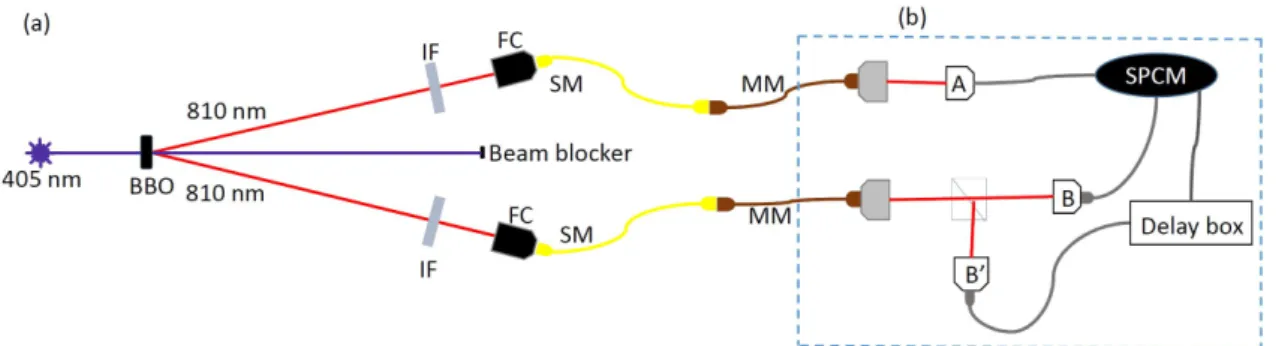
Spontaneous parametric down-conversion (SPDC) is a nonlinear process in which light of one fre-quency is converted into light of a different frefre-quency. In the process of SPDC a single photon of one frequency is converted into two photons of lower frequency. The input wave is referred to as the pump and the two outputs are referred to as the signal and idler. A type I SPDC process is considered here, where the signal and idler photons have the same polarization but orthogonal to
that of the pump. Conservation of energy requires that
ωp =ωs+ωi, (2.43)
whereωpis the frequency of the pump,ωsis the frequency of the signal andωiis the frequency of
the idler. Conservation of momentum requires that
kp=ks+ki, (2.44)
where kp,ks and ki are the pump, signal, and idler wavevectors respectively. Equations (2.43)
and (2.44) are known as the phase-matching conditions. For a type I process the interaction Hamil-tonian is ˆHI = ~ηaˆ†saˆ † i +H.c, where ˆa † s and ˆa †
i are the creation operators of the signal (s) and idler
(i) beams, respectively. The Hamiltonian represents a post-selection of the momenta of the output beams. The factorηis proportional to the classical field amplitude of the pump and the second order susceptibility of the nonlinear material. The signal and idler modes must emerge from the crystal on opposite sides of concentric cones centered on the direction of the pump beam as shown in Fig. 2.2a. Consider the initial state of the signal and idler modes to be represented by|Ψ0i=|0is|0ii, which is the vacuum state for type I down-conversion. The state vector evolves according to
|Ψ(t)i=e−
itHIˆ
~ |Ψ0i, (2.45)
which is expanded, since ˆHIhas no explicit time dependence, as
|Ψ(t)i ≈ 1− itHˆI ~ + 1 2 −itHˆI ~ !2 |Ψ0i (2.46)
to second order in time. For type I SPDC then we have
|Ψ(t)i= 1− µ
2
2
!
|0is|0ii−iµ|1is|1ii, (2.47)
whereµ=ηt. By detecting a photon in the idler (i) mode, a second term which has a single photon in the signal mode is selected. We can also detect a pair of photons, which also select out the second term, but this time there are two photons to work with as shown in Fig. 2.2.
2.3.2 Theory
In a classical field the correlations between the beam intensities,IBandIB0 is given by the degree
measurements [64]. It is given by g(2) B,B0(τ)= hIB(t+τ)IB0(t)i hIB(t+τ)ihIB0(t)i , (2.48)
whereIBandIB0are intensities detected by detectorsBandB0. It is called the degree of second-order
coherence because it involves correlations between intensities. When taking intensity measurements atτ= 0, for a 50:50 beam splitter in which theIB,IB0, and incident intensityI have the following
relationIB(t)= IB0(t)= 1 2Ii(t), then g(2)B,B0(0)= h[Ii(t)]2i hIi(t)i2 =g(2)(0). (2.49)
Using the Cauchy-Schwartz inequality [65]
g(2)
B,B0(0)=g
(2)(0)≥1. (2.50)
In quantum theory, the correlations between the output fields from the beam splitter are described by the quantum degree of second-order coherenceg(2)B,B0(τ). The electric fields and intensities are treated
as quantum mechanical operators. By taking measurements atτ=0, the detection of photons at the outputs quantum mechanically results in
g(2)B,B0(0)=
h: ˆIBIˆB0 :i
hIˆBihIˆB0i
, (2.51)
where the colons denote normally ordered operators with all creation operators to the left and anni-hilation operators to the right. The intensity operator is proportional to the photon number operator for the field ˆn=aˆ†aˆ, so that
g(2)B,B0(0)= hnˆBnˆB0i hnˆBihnˆB0i = haˆ†Baˆ†B0aˆBaˆB0i haˆ†BaˆBihaˆ†B0aˆB0i . (2.52)
Using beamsplitter transformations of the idler mode the second-order quantum coherence can now be composed as [65]
g(2)B,B0(0)=
hnˆi(ˆni−1)i
hnˆii2
=g(2)(0). (2.53)
The second-order coherence between the beam splitter outputs is equal to the second-order coher-ence of the input. Experimentally,g(2)at zero time delay is written as
g(2)(0)= NABB0NA
NABNAB0
Figure 2.2: Single photon source experimental setup.
whereNABB0 is the number of threefold coincidences,NABis the coincidence rates between
detec-tors A and B,NAB0 is the coincidence rate between detectors A and B’ and NA is the number of
single counts at detector A. There is a coincidence window that determines whether the detections are coincident. In the event that a genuinely single-photon state enters the beam splitter, the an-ticipated result would be thatg(2)(0) = 0, but this is not the case in an experiment. An outcome of characterizing a coincidence with an infinite time window is a nonzero second-order coherence function. This is on the grounds that there is the likelihood that uncorrelated photons from various downconversion events may hit the B and B’ detectors inside the infinite incident window; these are accidental coincidences.
2.3.3 Experimental Setup
Pairs of horizontally polarized single photons at 810 nm are produced by using a vertically polarized 200 mW solid-state laser (COHERENT OBIS) of peak wavelength 405 nm focused onto a Beta Barium Borate (BBO) concatenated crystal cut for type-I SPDC. Phase matching conditions lead to photons from a given pair being emitted into antipodal points of a forward directed cone with an opening angle of 6◦[90, 91]. Filters at 800 nm are placed on both paths (∆λ=40 nm) before each fiber coupler (FC) to spectrally select out the down-converted photons. The FCs consists of a 20x microscope objective and XYZ-translation stage. Such broad filters are used in order to maximize the generation rate of photon pairs for probing the plasmonic waveguides. While this influences the spectral quality of the photons, it is shown later that a second-order correlation value well below 0.5 is achieved, which is a clear indication that the experiments are performed in the single-photon regime. After the filters, each beam from the SPDC is sent to a single-mode fiber (SM).
NA(103cps) NB(103cps) NB0(103cps) NAB(102cps) NAB0(102cps) NABB0(102cps)
99 97 126 5 6 0.002
Table 2.1: Count rate results at zero time delay.
One of the SM fibers is connected to a multimode (MM) fiber which is directly connected to a single-photon silicon avalanche photodiode detector (SAPD Excelitas SPCM-AQR-15 labelled as A) which monitors the arrival of one photon from a given SPDC pair. A detection of a photon at the SPAD heralds the presence of a single photon in the other fiber [90]. The single-mode fiber on the other arm is in the same way connected to a MM fiber. The heralded photons from this fiber are sent to the HBT interferometer such that the correlations between photo-detections at SPAD detectorsB
andB0 are measured. The signal from detector B is sent to an electronic delay box circuit which make it possible to select the zero time delay required to take the measurement. Extra lengths of cabling are used to delay the signals from detectors A and B making it possible to set negative time delays (B0 arrives beforeAandB) using the delay circuit. Measurements were taken at zero time delay to record 12 runs with an integration time of 5 s per run and a coincidence window of 8 ns.
2.3.4 Results
Table 2.1 shows the count rates at zero time delay produced by a single-photon source. When the count rates and coincidence window increases, the number of accidental coincidences also increases. Equation (2.54) was used to calculateg(2)(0) values. The average value ofg(2)(0) was 0.1±0.04, which violates the classical inequalityg(2)(0)≥ 1 and it is lower than 0.5. This shows that single-photon excitations were achieved.
Chapter 3
Probing Decoherence in Plasmonic
Waveguides in the Quantum Regime
3.1
Introduction
In this chapter we experimentally investigate amplitude and phase damping for single SPPs in waveguides1. We refer to both types of damping as ‘decoherence’ because amplitude damping also reduces the coherence properties of single excitations [30, 70]. For the dimensions of the gold stripe waveguides we use, as depicted in Fig. 3.1 (a), the spatial mode is well defined as a sin-gle mode [71–74], with the SPPs excited in the number state degree of freedom. As a result, the decoherence is in the temporal domain as the SPP propagates. We probe plasmonic waveguides of varying lengths in a Mach-Zehnder interferometer configuration that has previously been used to study decoherence in atomic [76–80], electronic [81–83], photonic [84, 85] and relativistic [86] quantum systems. The configuration allows us to extract out values for the two main damping mech-anisms of the SPP system, as depicted in Fig. 3.1 (b): the amplitude damping time,T1– the time it
takes for the probability of an SPP in the excited state to reduce to 1/eits initial value – and the pure phase damping time,T2∗– the time it takes for the off-diagonal elements of an SPP state to reduce to 1/etheir initial values. The total phase damping time,T2, for a single SPP includes contributions
from bothT1 andT2∗, and is given by the relationT2−1 = T1−1/2+T2∗ −1,i.e. T2 ≤2T1 [30], where the presence ofT1 is a result of amplitude damping also contributing to total phase damping. In
our experiment we find values ofT1 = 1.90± 0.01×10⁻¹⁴ s, T2∗ = 11.19±4.89×10⁻¹⁴ s and thereforeT2 =2.83±0.32×10⁻¹⁴s. These suggest that the total phase damping time is dominated
by amplitude damping, showing that loss of amplitude is the most important factor in the
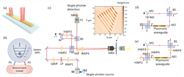
Figure 3.1: Experimental setup for probing the decoherence of single surface plasmon polaritons (SPPs).(a)Pictorial representation of the type of plasmonic waveguide probed. An input grating is used to couple single photons into the plasmonic waveguide, creating single SPPs which propagate along the waveguide, and then decouple back into single photons at an output grating.(b)Diagram showing two main damping channels for the waveguides – amplitude damping (AD) and phase damping (PD) – and their effect on the internal number state of the bosonic SPP: AD causes a loss of energy and reduces coherence (red arrows), while PD maintains energy but reduces coherence (blue arrows).(c)Microscope stage for probing the waveguides in configuration B. Configuration A does not include half wave-plate 2 (HWP2), the polarising beamsplitter (PBS) and the 50:50 beamsplitter (BS) - see main text for details. Inset shows a three-dimensional atomic force microscope image of the different length gold stripe waveguides used. (d)A Mach-Zehnder interferometer (MZI) for probing phase damping. (e)A modified version of the MZI with a polarizing beamsplitter, as used in the microscope stage.
herence of single SPPs in the plasmonic waveguides. However, the role of pure phase damping is not completely negligible. Our work shows that both amplitude and pure phase damping can lead to decoherence in quantum plasmonic systems, and it provides useful information about the loss of coherence that should be considered when designing plasmonic waveguide systems for phase-sensitive quantum applications, such as quantum sensing [19–22] and quantum imaging [22, 23]. The techniques developed here for characterising decoherence in plasmonic waveguides may be useful for studying other plasmonic nanostructures, such as those used as nanoantennas [4], as unit cells in metamaterials [87, 88] and as nanotraps for cold atoms [89].
3.2
Experimental setup
The setup used to probe SPP decoherence is shown in Fig. 3.1c. 2Here, a microscope is used to convert single photons into single SPPs on plasmonic waveguides. Single photons generated via SPDC, as explained in Chapter 2. Minor changes are made to the experimental setup for SPDC; polarizing beamsplitters (PBSs) are positioned in the path of the down-converted beams to clean up the polarization of the photons and remove any light with vertical polarisation. In order to main-tain the polarization of the heralded photon while it is transferred to the microscope, a polarisation maintaining (PM) fiber is used.
Two main configurations of the setup shown in Fig. 3.1c are used in the experiment. We denote these as configuration A and configuration B. In configuration A, half-wave plate 2 (HWP2), the PBS and the beamsplitter (BS) are not present. In this case, single photons are introduced to the stage via the beam expander (BE). Then, HWP1, a linear polarizer (LP) and a quarter-wave plate (QWP) are used to control the polarisation of the photons and maintain them as linearly polarized. HWP4 is used to optimize the polarisation for coupling the single photons into single SPPs on the waveguides [32]. A microscope objective (100x) focuses the beam of single photons onto the input grating of a plasmonic waveguide, as depicted in Fig. 3.1a. Excited single SPPs then propagate along the waveguide and are decoupled back into photons at an output grating. The microscope collects the decoupled photons, which are picked offby a knife-edge mirror (KM) and directed to a multimode fiber (MM) via a fiber coupler (FC). The MM fiber is connected to a SPAD. A detection of a photon together with a detection of the corresponding heralding photon from the SPDC pair within a coincidence window of 8 ns confirms single photons were sent through the microscope stage, converted to SPPs and then back into photons again.
In configuration B, which is used for a number of measurements, all components shown in Fig. 1c are present. These enable the quantification of the impact of waveguide propagation on the co-herence properties of single photons converted into SPPs. In this configuration, the microscope becomes part of one arm in a Mach-Zehnder interferometer (MZI) by using the PBS and BS, with one path photonic and the other plasmonic. Details of configuration B will be described later.
2Jason Francis contributed by designing the microscope stage for probing SPPs and data collection. Xia Zhang contributed by providing the atomic force microscope images and data collection.
The plasmonic waveguides probed have a range of different lengths, from 7.32 µm to 32.47 µm. They are gold stripes 2µm wide and 70 nm high. At the ends of the waveguides are gratings of height 90 nm made from 11 steps of period 740 nm, serving as inputs and outputs for converting photons to SPPs and back again [31]. Due to the design of the gratings, the optimal angle for in-coupling a photon is normal to the waveguide surface. Furthermore, due to reciprocity, the photons output from a grating at the end of a waveguide are also normal to the waveguide. This enables the insertion and collection optics in our setup to all be placed on the same side of the waveguide sample. The waveguides are fabricated as follows3. First, a positive photoresist is spin-coated on a silica glass substrate (refractive index 1.526), and then electron beam lithography is used to define the waveguide regions. Finally, a lift-offtechnique is used, with an adhesion layer of Ti (thickness 2-3 nm) followed by a 70 nm Au layer deposition using electron beam evaporation. The gratings are formed on the top in a similar process, utilising alignment marks to match the layers. A 3D image of the waveguides has been obtained using an atomic force microscope (NT-MDT Smena), as shown in the inset of Fig. 3.1c.
3.3
Results
We start with the results for amplitude damping of single SPPs using the microscope stage in config-uration A,i.e.without the MZI (HWP2, PBS and BS removed). Recent experiments have confirmed the bosonic nature of SPPs [92–96], and explored related quantum behaviour [97]. Initial results have also been obtained for amplitude damping of single SPPs [31]. Here, we confirm these results and provide a more detailed analysis of the role of amplitude damping in the decoherence process. We then investigate phase damping of single SPPs, which to our knowledge has not been done be-fore. The study of amplitude and phase damping at the same time allows us to combine both into a general model for decoherence of single SPPs. In Fig. 3.1b we show the energy level structure for a system of a bosonic particle (the SPP) [65]. Amplitude damping is associated with energy loss and the system, initially in an excited state|1i, will decay to the ground state|0iafter some timet
through its interaction with the environment. For the SPP this arises from electron collisions in the supporting metal which cause energy loss in the electronic degree of freedom of the SPP, as well as surface defects and the mode structure of the waveguide causing energy loss in the optical
gree of freedom due to coupling of light into the far-field. In general, for single bosonic excitations undergoing amplitude damping we have the following transformation of the density matrix for the system, ρ(0)→ρ(t)= ρ00+(1−e−Γ1t)ρ11 e−Γ1t/2ρ01 e−Γ1t/2ρ10 e−Γ1tρ11 , (3.1)
where ρi j = hi|ρ(0)|ji are the initial entries of the density matrix at t = 0 in the number state
basis,|ni, and Γ1 characterizes the strength of the damping induced by the environment [30]. In
the classical regime,Γ1corresponds to population decay or loss, the value of which is easily found
by measuring the decay of the SPP intensity as a function of waveguide length. Here, the length at which the intensity has dropped to 1/e of its initial value is the propagation length L [1], and the value forΓ1is then the inverse of the time at which the SPP reaches this length (T1), given by
Γ1=vg/L, wherevgis the group velocity of the SPP. In the quantum regime, when single SPPs are
considered, the value ofΓ1can be found similarly, but the intensity measurement is replaced by the
mean single-excitation count rate [31, 32]. This can be obtained in our setup by measuring the rate of coincidences between the heralding photon and the photon that has undergone the photon-SPP-photon conversion process, as the waveguide length increases. A coincidence detection corresponds to the case where a single photon was generated, converted to a single SPP and then converted back to a single photon. The length at which the coincidence rate drops to 1/eof its initial value is then the propagation length L in the single-SPP regime. It represents the length at which the probability of an excited single SPP to propagate to that point reduces to 1/e [31]. The value forΓ1 is then
obtained as in the classical case. To check that we are able to probe single SPPs in the waveguides we measure the second-order correlation functiong2(0) for single photons sent through a waveguide of length 7.47 µm, as described in Ref. [31]. We find g(2)(0) = 0.26±0.01, which is below 0.5, confirming we are in the single-excitation regime [65]. This value ofg(2)(0) is larger than that of the photon source. This is due to the low count number and the stability of the setup over the period in which the counts are recorded. The impact of the grating on filtering the frequency affects the spectral purity of heralded photon.
We first measure the propagation length L using the microscope in configuration A in the clas-sical regime using a white laser source (Fianium WL-MICRO) and a filter centered at 810 nm with ∆λ = 10 nm. The input intensity is set to a few mW and the transmitted light intensity (104−105cps) is recorded by an SPAD coupled to a MM fiber, as shown in Fig. 3.1 (c). The results for different waveguide lengths are shown in Fig. 3.2 (a). One can clearly see the well-observed
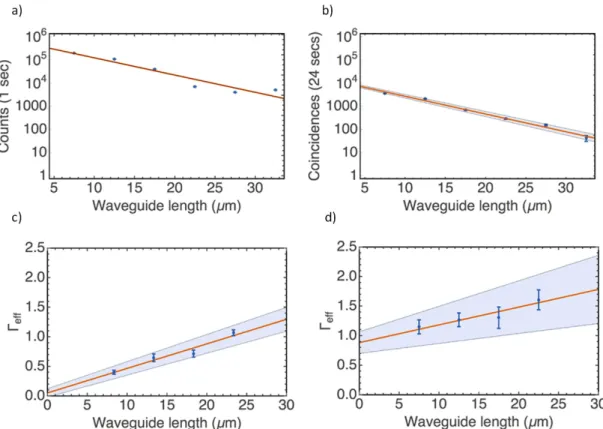
Figure 3.2: Decoherence in the classical and quantum regime.(a)Intensity throughput as a function of waveguide length showing amplitude damping for classical SPPs. (b) Amplitude damping for single SPPs in the quantum regime measured via coincidences with a heralding photon.(c)Effective
phase damping parameterΓe f f as a function of waveguide length showing pure phase damping for
classical SPPs.(d)Effective phase damping parameterΓe f f showing pure phase damping for single
SPPs. The shaded regions represent upper and lower values of a straight line best fit using the least squares method and a Monte Carlo simulation drawing each data point from within its individual standard deviation with Poissonian distribution.
exponential decay of the intensity as the waveguide length increases. We find a propagation length ofL=5.85±0.03µm. Which is determined by the best fit to exponential decay shown in Fig. 2a via a least squares method and extracting the 1/evalue. This value is similar to previous experimental work [28, 31], although slightly smaller than the 10µm predicted using finite element simulation (COMSOL) of the stripe waveguide [71–74]. The difference may be caused by edge effects along the lateral width of the waveguides, surface and material defects during fabrication, and a small deviation of the actual dielectric function of gold from that used in the simulation [75]. COMSOL’s 2D mode silver model was used to solve for modes supported by the stripes. The solution gives the full fields and complex effective mode index (which was used to calculate vg). The geometry
of the system was the 2D cross-section of the waveguide. The mesh has a minimum element size of 0.1 nm everywhere and a maximum element size ofλ0/25 for the waveguide and surrounding
7.0×10⁶ 8.0×10⁶ 9.0×10⁶ 1.0×10⁷ 1.1×10⁷ 1.2×10⁷ 1.3×10⁷ 2.5×10¹⁵ 3.0×10¹⁵ 3.5×10¹⁵ k0(m-1) ω ( Hz )
Figure 3.3: Dispersion curve for light in a stripe waveguide.
region extending 250 nm from the waveguide surface. The maximum element size elsewhere is λ0/5. Hereλ0is the free-space wavelength of 810 nm corresponding to the SPP.
To convert this to the amplitude damping timeT1we obtain the SPP dispersion relation for the
plas-mon mode in the waveguide from the simulation shown in Fig. 3.3. Based on this, we find the group velocityvg(ω0)=2.958×10⁸ms−1at the free-space wavelengthλ0=810 nm. From the simulation
kas a function ofω,vg(ω0)=
∂k
∂ω
−1
at a givenω0. A more rigorous approach would be to directly
measure the group velocity; however, for the waveguide dimensions and free-space wavelength we consider, theoretical simulation describes the experimental data well [73]. Furthermore, here we use the group velocity simply to convert the damping factor into the time domain and its value in the spatial domain is valid regardless. Using the group velocity we findΓ1=5.06±0.01×10¹³s−1
and an amplitude damping time ofT1 = Γ−11 =1.98±0.01×10⁻¹⁴s.
In Fig. 3.2 (b) we show the results for single SPPs in our experiment. Here, the exponential decay of the mean count rate (observed via the coincidence rate) is seen as the waveguide length increases. The data collection time has been increased to 24 s for each length in order to measure a simi-lar number of counts as the classical case, which has a shorter collection time of 1 s. We find a propagation length of L = 5.61± 0.05 µm, consistent with the result from the classical regime.
From this we obtainΓ1 = 5.27±0.02×10¹³ s−1 and a single-SPP amplitude damping time of
T1 = Γ−11 = 1.90±0.01×10⁻¹⁴ s. In general, the relation between the phase damping timeT2
and amplitude damping timeT1is given byT2−1 =T1−1/2+T2∗ −1[30], whereT2∗is the pure phase
damping time. Thus, from the above result we already have an upper bound ofT2 ≤2T1for single SPPs in the quantum regime. However,T2∗remains to be found to determine the exact value ofT2,
and could reduce it appreciably.
Pure phase damping characterized by the timeT2∗ is associated with interactions where energy is maintained and therefore a system initially in a ground state, or excited state, will remain in that state after some timet. However, a state in a superposition of ground and excited states will experience a loss of coherence between the states due to a time varying change in the relative phase. For the SPP this arises from electron collisions in the supporting metal associated with elastic processes [38,69]. For single bosonic excitations we have the following transformation of the density matrix,
ρ(0)→ρ(t)= ρ00 e−Γ ∗ 2tρ01 e−Γ∗2tρ10 ρ11 , (3.2)
whereΓ∗2characterizes the strength of the damping induced by the environment [30]. In the classical regime,Γ∗2corresponds to the loss of temporal coherence. We obtain its value in the classical and quantum regime by placing different length plasmonic waveguides inside a MZI and measuring the loss of interference between the two paths, as shown in Fig. 3.1 (d). In what follows, we describe how this is done in the quantum regime and link it with the classical case in the corresponding limit.
We start with the case of no decoherence in the waveguides. In Fig. 3.1 (d) we consider the input state|0i1|1i2, corresponding to a single photon in mode 2. The first beam splitter (BS1) transforms the state to [65]
1
√
2(
|0i10|1i20+i|1i10|0i20). (3.3)
Taking the neutral density (ND) filter and plasmonic waveguide as having unit transmission for the moment, and the mirrors (M1 and M2) contributing a phase factoreiπ/2to each term, we have the following state after the second beamsplitter (BS2),
1 2[(1−e
i(φ−δ))|0i
100|1i200+i(1+ei(φ−δ))|1i100|0i200]. (3.4)
translation stage and the phaseδ = kspp`, withkspp the SPP wavenumber and` the length of the
plasmonic waveguide. The probability of a photon detected in mode 100is then simply
p(φ)= 1
2(1+cos(φ−δ)). (3.5) We now introduce decoherence in the system. When amplitude and pure phase damping are in-cluded in the plasmonic waveguide, the transformations in Eqs. (3.1) and (3.2) are applied to the state after the first beamsplitter, given by Eq. (3.3). The transformations are given explic-itly for mode 20 by |0i h0| → |0i h0| +(1 −e−Γ1t)|1i h1|,|0i h1| → e−Γ∗2te−Γ1t/2|0i h1|,|1i h0| → e−Γ∗2te−Γ1t/2|1i h0|and|1i h1| → e−Γ1t|1i h1|. The probability of a photon detected in mode 100then
becomes
p(φ)= 1 4(1+e
−Γ1˜ +
2e−Γ1˜ /2−Γ˜∗2cos(φ−δ)), (3.6)
where ˜Γ1 = Γ1`/vg = `/Land ˜Γ∗2 = Γ∗2`/vg. As ˜Γ1 is already known from previous measurements
andδis a fixed phase for a given waveguide length`, then by measuring p(φ) asφis varied using the translation stage of M1, the remaining unknown parameter ˜Γ∗2can be extracted to obtainΓ∗2, and thusT2∗. In practice, however, the impact of amplitude damping in the plasmonic waveguide reduces the average value ofp(φ) significantly and in the most extreme case we have p(φ) = 1/4, as only photons going through the free-space arm of the MZI will be detected. As the amplitude damping in the plasmonic waveguide becomes large it is difficult to observe oscillations inp(φ) and extract out ˜Γ∗2. This problem can be addressed by introducing an additional tuneable amplitude damping on the free-space arm using a variable neutral density (ND) filter. As the photon is also a boson, we can use Eq. (3.1) to model the damping, which changes the probability of detection to
p(φ)= 1 4(e
−Γ+
e−Γ1˜ +2e−(Γ+Γ1˜ )/2−Γ˜∗2cos(φ−δ)), (3.7)
whereΓcharacterizes the amplitude damping on the free-space arm. This parameter can be tuned to match ˜Γ1in the plasmonic waveguide by blocking the plasmonic waveguide arm and measuring
the output counts in mode 100as the ND filter is varied.
In order to integrate the MZI of Fig. 3.1 (d) into our microscope stage more easily we replace BS1 and the variable ND filter with a PBS preceded by HWP2, as shown in Fig. 3.1 (e). This configuration provides polarization control over the relative splitting into modes 10 and 20, and allows us to increase the rate of photons injected into the plasmonic waveguide compared to the original configuration of Fig. 3.1 (d). HWP4 provides polarization control for optimising coupling
of single photons to single SPPs and HWP3 rotates the polarization of the free-space arm to match the output of the plasmonic beamsplitter in order to obtain interference at the BS. For a given waveguide length, once HWP3 and HWP4 have been modified, the polarization state in the free-space and plasmonic arms is fixed for the entire set of measurements. The above modifications change the detection probability to
p(φ)= 1 2(e
−Γ10 +
e−( ˜Γ1+Γ20)+2e−(Γ10+Γ20+Γ1˜ )/2−Γ˜∗2
cos(φ−δ)), (3.8) whereΓ10 andΓ20 are controlled by HWP2, and we setΓ10 = Γ˜1+ Γ20 in order to observe clearly
a symmetric oscillation in p(φ). Finally, we include a possible asymmetry in the splitting at the BS, which has an order of magnitude larger error in its splitting than the PBS. With reflection and transmission coefficientsR andT, respectively, for the BS, this changes the detection probability to
p(φ) = R e−Γ10
+T e−( ˜Γ1+Γ20)
+2√RT e−(Γ10+Γ20+Γ1˜ )/2−Γ˜∗
2cos(φ−δ). (3.9)
From the above equation it would appear that only a single waveguide length is needed to extract out ˜Γ∗2. However, in practice it is not always possible to get a complete overlap of modes 10 and 20 at the BS. This non-ideal overlap reduces the visibility of the oscillations in p(φ) and acts as an effective phase damping, which we describe using the parameterΓint. Thus, ˜Γ∗2 in Eq. (3.9) is
transformed as ˜Γ∗2→Γeff =Γ˜∗2+Γint. Due to this non-ideal overlap, it appears that we must also find Γintto obtain ˜Γ∗2. This can be done by extractingΓeff fromp(φ) for waveguides of different lengths
and then usingΓeff(`) = Γ∗2`/vg+ Γint, where the pure phase damping per unit length,Γ∗2/vg, is the
gradient ofΓeff(`) andΓintis they-intercept.
In Fig. 3.2 (c) and (d) we plotΓeff(`) for increasing waveguide length in the classical and quantum
regime, respectively. For the classical case,Γeff(`) is obtained by fitting the functionI(φ)= Iinp(φ)
to intensity measurements, whereIin is the initial input intensity to the MZI. Examples of the
in-tensity measurements for the different waveguide lengths probed in the classical regime are shown in Fig. 3.4 (a)-(d) over a period of oscillation. A Monte Carlo simulation is carried out for each of these figures, whereΓeff(`) is varied to fit the functionI(φ) for 200 instances of a given figure.
Each instance has its data points drawn randomly from within the standard deviations measured at each value ofφusing a Poissonian distribution. All other parameters ofI(φ) are known except
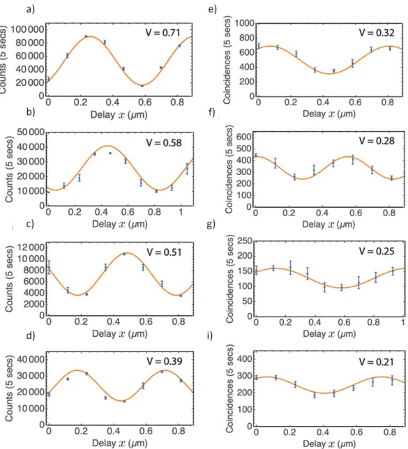
Figure 3.4: Intensity dependence of the output signal from the MZI in the classical and quantum regimes for different waveguide length as the phase φis modified. Here, φ = 2πsx/λ0, where s
accounts for the translation stage geometry andx is its position×2 (total delay). (a)-(d)The left hand column corresponds to the classical regime with intensity measured as counts. (e)-(h)The right hand column corresponds to the quantum regime with intensity measured as coincidences. The solid lines are fits usingp(φ). The length of the waveguide increases with row number in steps of 5µm and is 8.31µm, 13.31µm, 18.31µm and 23.31µm for the left hand column and 7.47µm, 12.47µm, 17.47µm and 22.47µm for the right hand column. The visibility is given in the inset for each panel and related to system parameters byV =(pmax−pmin)/(pmax+pmin). Maximum counts do not necessarily decrease as the length increases due to variations in alignment and intensity optimized for each waveguide.
for Γeff(`), and the resulting values extracted are shown in Fig. 3.2 (c). The error bars on each
length`. From Fig. 3.2 (c) we find a gradient ofΓ∗2/vg= 0.042±0.003 (µm)−1and thus a value of Γ∗ 2=1.25±0.11×10 13s−1andT∗ 2 =8.03±0.71×10 −14s.
It should be noted that the periods of the oscillations shown in Fig. 3.4 are not all equal to the wavelength of the single photons (810 nm). The change in the period is due to small differences in the angle of the output beam for different length waveguides. Although the output beams from the gratings are designed to be normal to the waveguide surfaces, small differences in the lateral beam displacement due to the different length of the waveguides results in an angle change when the beams pass through the microscope objective. The result is that the delay distance x that the mirror stage moves is rescaled by a small geometric factors, becomingsx. The change in period does not have any effect on the values of the decay parameters extracted from the fits as these are dependent only on the amplitude and mid-point of the oscillations.
In Fig. 3.2 (d) we perform the same extraction method for single SPPs and Fig. 3.4 (e)-(h) shows examples of the oscillations used for each waveguide length. From Fig. 3.2 (d) we find a gradient of Γ∗2/vg = 0.030± 0.013 (µm)−1 and thus a value of Γ∗2 = 0.89± 0.39× 10¹³s−1 and T2∗ =
11.19±4.89×10⁻¹⁴s. While the results from the quantum case are clearly statistically more noisy, the values are consistent with those found in the classical regime to within a standard deviation. It is also interesting to inspect the values ofΓint, which are found to be 0.048±0.061 and 0.893±
0.193 for the classical and quantum case, respectively. The difference in values is due to the better mode overlap achieved in the classical case, as the interference could be optimized by monitoring the intensity fluctuations with a spectrometer in real-time and with a reduced bandwidth for the source of light. Indeed, one can see the better mode overlap via the high visibility of the oscillations in the classical case in Fig. 3.4 (a). For the quantum case, due to the low count rates real-time monitoring could not be performed and a similarly good mode overlap was not possible. The low count rates are also the cause of the larger error bars in Fig. 3.2 (d), as the statistical fluctuations are larger due to the instability of the MZI over the longer time periods required for data collection. The single-SPP amplitude damping measurements shown in Fig. 3.2 (b) do not require the MZI and thus have smaller error. Improvements to the generation rate of our single-photon source would allow an increase in visibility and reduction in the error in the phase damping investigation. It would also allow the probing of longer waveguides. However, even with the current setup we are able to observe the same trend ofΓeff in the quantum regime as seen in the classical regime.
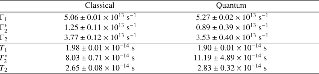
Classical Quantum Γ1 5.06±0.01×10¹³s−1 5.27±0.02×10¹³s−1 Γ∗ 2 1.25±0.11×10¹³s −1 0.89±0.39×10¹³s−1 Γ2 3.77±0.12×10¹³s−1 3.53±0.40×10¹³s−1 T1 1.98±0.01×10⁻¹⁴s 1.90±0.01×10⁻¹⁴s T2∗ 8.03±0.71×10⁻¹⁴s 11.19±4.89×10⁻¹⁴s T2 2.65±0.08×10⁻¹⁴s 2.83±0.32×10⁻¹⁴s
Table 3.1: Summary of results from probing decoherence in plasmonic waveguides.
An important factor that might influence our measurement of pure phase damping is dispersion in the plasmonic waveguides. For large dispersion, the SPP wavepacket would spread significantly and any interference between the photon it is converted into and the free-space photon would be reduced, and appear as phase damping. In order to assess the impact of this effect, we calcu-late the group velocity dispersion (GVD) coefficient, defined as Dω0 =
d
dω(vg1(ω))|ω0 [98]. Using the dispersion relation for the plasmonic waveguides from the mode simulation [71–74], we find
Dω0 = 5.81× 10
−25 s/m-Hz. To see how this affects the interference, as an example we take
an initial Gaussian wavepacket spectral amplitude for a single SPP centred on ω0 as ξ0(ω) =
(2πσ2ω)−1/4e−(ω−ω0)2/4σ2ω, where a single SPP is described as 1ξ
E
= R
dωξ0(ω)ˆa†(ω)|0i [32, 65].
The initial temporal spread isσt0 = 1/2σω. After timet, the wavepacket has moved a distance`
and spread according toσt = (σ2t0 +(`Dω0/2σt0)
2)−1/2. We then have the corresponding spectral
amplitudeξt(ω) = (2πσ2ω,t)−1/4e
−(ω−ω0)2/4σ2ω,t, withσω,t = 1/2σt. Calculating the overlap ofξ0(ω) andξt(ω) gives a quantity that represents how well the mode from the plasmonic waveguide
over-laps with the free-space photonic mode at the BS in the MZI [99]. Here,ξ0(ω) represents the photon
in the free-space mode (negligible dispersion) andξt(ω) represents the photon from the plasmonic
waveguide (with dispersion). Setting σω = ∆ω/2√2ln2, with ∆ω corresponding to a FWHM of ∆λ = 40 nm, and takingω0 corresponding to the central wavelength λ0 = 810 nm and using the
GVD coefficient together with a length` = 90µm (more than 3 times the longest waveguide con-sidered), we findR ξ∗0(ω)ξt(ω)dω = 0.99. Thus it is expected that there is a negligible impact of
dispersion on the interference for the waveguide lengths considered.
We now combine all the results in this study, taking the amplitude damping and pure phase damping values found. The combined phase damping time isT2 =(T1−1/2+T2∗ −1)−1=2.65±0.08×10⁻¹⁴s
and 2.83±0.32×10⁻¹⁴s in the classical and quantum regimes, respectively. We are therefore able to confirm that in both cases, amplitude damping is the main source of phase and amplitude decay in
the plasmonic waveguides, although pure phase damping modifies the phase damping by a relatively small amount. A summary of the main results of the study is given in Tab. 3.1.
3.4
Discussion
In this Chapter we investigated the decoherence of SPPs in plasmonic waveguides in the classical and quantum regimes. We measured both amplitude and phase damping effects of SPPs. We found that for classical SPPs and single SPPs, amplitude damping is the main source of amplitude and phase decay. The results will be useful in the design of phase-sensitive quantum plasmonic applica-tions, such as quantum sensing and allow appropriate quantum states to be chosen for a given task to be achieved. While our work has been limited to probing decoherence for single excitations of SPPs in the quantum regime and many excitations in the classical regime, there is an intermediate regime, involving low numbers of excitations that remains to be investigated. It would be interest-ing to confirm the role of decoherence in this regime, where the bosonic SPP mode is treated as a qudit [100]. This would be important for developing quantum plasmonic state engineering at the few SPP excitation number.