Civil and Environmental Engineering Faculty
Publications and Presentations
Civil and Environmental Engineering
4-2016
Estimating River Discharge Using Multiple-Tide Gauges
Distributed Along a Channel
Hamed R. Moftakhari
Portland State University
, [email protected]
David A. Jay
Portland State University
, [email protected]
Stefan Talke
Portland State University
, [email protected]
Let us know how access to this document benefits you.
Follow this and additional works at:
https://pdxscholar.library.pdx.edu/cengin_fac
Part of the
Civil Engineering Commons
,
Environmental Engineering Commons
, and the
Hydraulic Engineering Commons
This Article is brought to you for free and open access. It has been accepted for inclusion in Civil and Environmental Engineering Faculty Publications and Presentations by an authorized administrator of PDXScholar. For more information, please [email protected].
Citation Details
Moftakhari, H. R., D. A. Jay, and S. A. Talke (2016), Estimating river discharge using multiple-tide gauges distributed along a channel, J. Geophys. Res. Oceans, 121, 2078–2097.
RESEARCH ARTICLE
10.1002/2015JC010983
Estimating river discharge using multiple-tide gauges
distributed along a channel
H. R. Moftakhari1, D. A. Jay1, and S. A. Talke1
1Department of Civil and Environmental Engineering, Portland State University, Portland, Oregon, USA
Abstract
Reliable estimation of freshwater inflow to the ocean from large tidal rivers is vital for water resources management and climate analyses. Discharge gauging stations are typically located beyond the tidal intrusion reach, such that inputs and losses occurring closer to the ocean are not included. Here, we develop a method of estimating river discharge using multiple gauges and time-dependent tidal statistics determined via wavelet analysis. The Multiple-gauge Tidal Discharge Estimate (MTDE) method is developed using data from the Columbia River and Fraser River estuaries and calibrated against river discharge. Next, we evaluate the general applicability of MTDE by testing an idealized two-dimensional numerical model, with a convergent cross-sectional profile, for eighty-one cases in which nondimensional numbers for fric-tion, river flow, and convergence length scale are varied. The simulations suggest that MTDE is applicable to a variety of tidal systems. Model results and data analyses together suggest that MTDE works best with at least three gauges: a reference station near the river mouth, and two upstream gauges that respond strongly to distinct portions of the observed range of flow. The balance between tidal damping and amplify-ing factors determines the favorable location of the gauges. Compared to previous studies, the MTDE method improves the time resolution of estimates (from 2.5 to<1 week) and is applicable to systems with mixed diurnal/semidiurnal tides. However, model results suggest that tide-induced residual flows such as the Stokes drift may still affect the accuracy of MTDE at seaward locations during periods of low river discharge.1. Introduction
The freshwater discharge to the ocean from large tidal rivers is an important component of the global water balance [Oki et al., 1995;Alsdorf and Lettenmaier, 2003], and its estimation is required for climate analyses and water resources management [Laize and Hannah, 2010; Loitzenbauer and Mendes, 2012]. Globally, changes in discharge affect chemical and sediment input to the ocean [Martin and Whitfield, 1983;Syvitski et al., 2003;Syvitski, 2003;Moftakhari et al., 2015a]. On a smaller scale, accurate river discharge measure-ments are necessary for assessing coastal inundation and planning navigation projects [Peng et al., 2004;
Prandle, 2000;Moftakhari et al., 2015b], as well as for analyses of coastal upwelling [Gan et al., 2009;Palma et al., 2006], beach sediment supply [Flick and Ewing, 2009;Inman and Jenkins, 1999], habitat access and res-toration [Kimmerer, 2002;Kukulka and Jay, 2003a, 2003b;Cloern et al., 1983], salinity intrusion [Prandle, 1985;
Uncles and Peterson, 1996; Cloern et al., 1989; Monismith et al., 2002], and the impacts of future climate change [Scavia et al., 2002;Syvitski, 2003].
Estimation of net freshwater discharge with conventional technology is difficult near the mouth of an estu-ary, for methodological reasons [Jay et al., 1997;Fram et al., 2007]. The reversing tidal flow, the compensa-tion flow for the tidal Stokes drift, spring-neap water storage effects, lateral circulacompensa-tion, estuarine circulacompensa-tion and the presence in some systems of multiple distributaries or separate ebb/flood channels make this esti-mation/measurement difficult [Buschman et al., 2010;Sassi et al., 2011b].Gisen and Savenije[2015] recently developed an empirical relationship between estuarine shape and freshwater inflow which can be used to determine bankfull river discharge in ungauged estuaries. However, the methodology is limited to fully allu-vial, undisturbed systems (i.e., with limited flow regulations and dredging) with semidiurnal tides, and excludes tidal inlets, bays, rias, fjords, sounds, and submerged river valleys. Several recent studies have introduced methods to calculate discharge in tidal rivers far from the mouth [Hoitink et al., 2009;Sassi et al., 2011a;Kawanisi et al., 2010;Chen et al., 2014]. However, these methods cannot capture downstream losses
Key Points:
Wavelets are used to estimate tidal river discharge from multiple tide gauges
Using tidal statistics provides better resolution and accuracy than other methods
Results are best in frictional, convergent estuaries with moderate to high flow Supporting Information: Supporting Information S1 Figure S1 Correspondence to: H. R. Moftakhari, [email protected] Citation:
Moftakhari, H. R., D. A. Jay, and S. A. Talke (2016), Estimating river discharge using multiple-tide gauges distributed along a channel,J. Geophys. Res. Oceans,121, 2078–2097, doi:10.1002/2015JC010983.
Received 18 MAY 2015 Accepted 26 FEB 2016
Accepted article online 1 MAR 2016 Published online 1 APR 2016
VC2016. American Geophysical Union. All Rights Reserved.
Journal of Geophysical Research: Oceans
PUBLICATIONS
due to infiltration, evaporation, and water diversion, or gains due to small tributaries, groundwater recharge, and storm water/sewer outfalls.
To address this problem, we note that tidal range decays upriver due to the effects of friction (due partially to river flow), producing a signal that can be calibrated to discharge measurements.Godin [1999] and
Kukulka and Jay[2003a, 2003b] suggested that the damping coefficient depends nonlinearly on river flow velocity.Sassi and Hoitink[2013] explained the mechanism of river-tide interactions as a mutual feedback between river stage and tidal motion. Their study suggests that even for high river flow and low tidal veloc-ity amplitudes, river-tide interaction contributes significantly to subtidal friction.
Moftakhari et al. [2013], using an approach first suggested byJay and Kukulka[2003], developed a method to estimate river discharge in an estuary using the perturbations in tidal constituents that occur due to non-linear frictional interaction between river flow and tides. Specifically, if astronomical or coastal tidal forcing is known, discharge may be estimated at a tide gauge via an inverse model that relates river flow to tidal damping or overtide generation. The tidal discharge estimate (TDE) is calibrated to available river flow measurements, and does not require direct flux measurements at the ocean entrance. For a gauge placed at the estuary inlet, the TDE method estimates net flow from the estuary to the ocean, easing estimation of freshwater inflow through complex deltaic or estuarine systems, particularly during times when no fluvial measurements are available. For locations where long time series of tide data are available [cf.Talke and Jay, 2013], the TDE method can capture changes in reservoir management, climate cycles and long-term hydrological trends that cannot easily be ascertained from other data sources [Moftakhari et al., 2013, 2015a]. However, though useful, the TDE method is based on simple dynamical ideas that neglect a number of potentially important factors such as neap-spring storage effects, the Stokes drift and variations in chan-nel cross section with river flow. The effects of these factors on flow estimates cannot be completely elimi-nated, but we show here that better estimates can be obtained using multiple gauges.
Cai et al. [2014] applied a one-dimensional, analytical tide model to investigate the influence of river dis-charge on tidal wave propagation and residual water level slope. Their study improved the prediction of the tidal propagation in estuaries (i.e., tidal damping, velocity amplitude, wave celerity and phase lag), and proposed an alternative analytical approach for estimating freshwater discharge on the basis of tidal water level observations along the estuary. Like TDE, theCai et al. [2014] approach assumes exponential conver-gence of the cross-sectional area, and that the river and tidal discharge be of similar magnitude. In addition, theCai et al. [2014] approach requires that the tides be predominantly semidiurnal.
To improve flow estimation, several attempts have also been made to eliminate tidal effects from river data.
Lim and Lye[2004] used a wavelet analysis to detide water level data, such that a conventional flow versus stage calibration could be applied.Pagendam and Percival[2015] detided stream velocity records in tidal riv-ers via a combination of robust harmonic analysis and Kalman filtering to directly derive river flow. How-ever, de-tiding a strongly nonstationary, tidally influenced, river discharge record is not trivial, and it is unclear whether this approach deals with the strong tidal monthly oscillations that are so prominent in large tidal rivers [Buschman et al., 2009;Jay et al., 2015], or are able to separate out the Stokes drift return flow from the river flow. Rather than detiding, our approach uses the river signal inherent in the tidal varia-tion to improve estimates of river discharge.
The purpose of this paper is to demonstrate the feasibility and utility of a multiple-gauge tidal discharge estimate (MTDE) method which uses wavelets to analyze nonstationary tidal properties at multiple locations along a tidal river. Compared to previous efforts, our method results in higher temporal resolution (i.e., less than a week), accounts for neap-spring storage effects, and eliminates some processes that affect discharge estimates, especially during low flow periods (e.g., nonlinear effects on tides from continental shelf and estuary entrance processes). We first develop and calibrate an MTDE model to the Columbia and Fraser River estuaries. These locations were chosen both based on the availability of high quality river discharge estimates, the availability of multiple tidal data sets (>10 years duration), and because these systems, with substantial semidiurnal and diurnal tides, are challenging tests of the method. To better understand the physical mechanisms behind MTDE and its applicability to other systems, we next develop an idealized two-dimensional (2D) numerical model using Delft3D Flow [Booij et al., 1999]. The model, with a convergent cross-sectional profile similar to many estuaries, is tested for 81 cases in which nondimensional numbers for friction, river flow, and convergence length scale are varied. Finally, we compare results of the analyses
from real systems with idealized model results from runs with the similar nondimensional numbers, in order to better understand mechanisms and sources of error.
2. Case Studies and Data Sources
2.1. Case StudiesThe Columbia and Fraser river estuaries (Figure 1a), in which MTDE is calibrated, together drain about 888,000 km2of North America and deliver an annual average of about 273,000 million cubic-meter (Mm3)
of freshwater to the Pacific Ocean, 2003–2013.
The Fraser River (FR), with an average discharge of 2700 m3s21, is the largest river on the west coast of Can-ada; because it has only one large dam, its flow cycle is one of the least anthropogenically altered in west-ern North America. The watershed above the river gauge at Hope (Figure 1b) provides about 72% of the freshwater flow to the ocean, while the rest of the discharge comes from the local tributaries close to its delta [Milliman, 1980]. The river flow is strongly seasonal and most of the discharge comes from melting snow between May and mid-July [Milliman, 1980]. The greater diurnal tidal range at the mouth is 4m during low-flow periods. During high-flow periods, greater diurnal tidal range decreases landward to about 0.1– 0.2 m at Port Mann (Figure 1b) [Milliman, 1980]. Tides are mixed diurnal (D1)-semidiurnal (D2) in this system,
with a D2/D1ratio of about 1. The total length of the system to the head of the tides is about 110 kilometer.
The Columbia River (CR), with an average flow of 7500 m3s21, is the fourth largest river in North America.
Climate change, flow regulation, and irrigation diversion have reduced the mean and peak flows, and
Figure 1.Map of the study area; (a) The watershed boundaries for Fraser river and Columbia River, and location of Figures 1b and 1c; (b) Fraser River estuary; (c) Columbia River estuary. Black dots represent the tide gauges, and black triangles represent the river flow observa-tories. The IDs for each gauge in the Fraser River are based on Canada Environment database, and in the Columbia River are on the NOAA and USGS databases. Copyright for ESRI and http://www.cec.org/.
altered the shape of its annual hydrograph over the last century [Naik and Jay, 2011]. The tide has a mixed character with a D2/D1ratio of 1.8 at the estuary mouth [Jay et al., 2011]. The greater diurnal tidal range in
the lower Columbia River varies from1.7 to 3.6 m at the ocean entrance and increases to a maximum of
2.0 to 4.0 m, at Astoria Tongue-Point (river-kilometer (RKM) 29; Figure 1c). Tidal amplitude then decreases monotonically, and tides are virtually undetectable at the most seaward dam at RKM 234 [Jay et al., 2011, 2014]. Tides in both the Columbia and Fraser River are nonstationary due to fluctuating river flow, and any description of their tidal properties in terms of conventional tidal constituents is approximate [Kukulkaand
Jay, 2003a].
The available data for multiple gauges along the channel, which are relatively complete over the past ten years for both estuaries, provide the chance to investigate the applicability of MTDE for different tidal char-acteristics (i.e., D2/D11 in Fraser versus D2/D12 in Columbia) and from a freshwater regime which is
heavily controlled (Columbia River) to one of the least anthropogenically altered systems in the North America (Fraser River).
2.2. Data Sources 2.2.1. Tide Data
Hourly water-level data for tide gauges located at Steveston (RKM 5), New Westminister (RKM 40), Port Mann (RKM 45) and Mission (RKM 82) in the Fraser River were obtained from Environment Canada, from 2000 to 2012 (Figure 1b). Hourly water-level data from 2002 to 2012 for the Columbia River estuary (Figure 1c) were downloaded from the National Oceanic and Atmospheric Administration (NOAA) website, and include tide gauges located at Astoria (RKM 29), Skamokawa (RKM 54), Wauna (RKM 68), Longview (RKM 107), St Helens (RKM 139), and Vancouver (RKM 172). Additional tide data at Beaver Army Terminal (RKM 87) were obtained from the US Geological Survey (USGS). The 2002–2012 period was chosen because data collected before March 2002 (available from regional sources) exhibit gaps, irregularities in timing, and datum shifts at some stations. For both systems, the water-level data are relatively (>96%) complete for all the gauges over the analysis period, and the chosen period is long enough to capture a large dynamic range of river flow conditions, including relatively low, moderate and high flow events.
2.2.2. Discharge Data
Environment Canada provides daily discharge estimates for the Fraser River at Hope (ID: 08MF005; Figure 1b) for a 104 year period starting in 1912. The watershed area above this gauge is about 217,000 km2, 93% of the total basin area. We use the daily observed flow at this gauge as representative of freshwater enter-ing the lower Fraser estuary, recognizenter-ing that it does not record flows from tributaries further downstream, about 28% of the total discharge to the ocean.
The daily discharge values observed at Beaver Army Terminal, near Quincy, OR (USGS 14246900; Figure 1c) best represents the freshwater inflow to the lower Columbia River estuary. The watershed area above this gauge is665,000 km2; it drains99% of the Columbia River watershed, and captures97% of the total
discharge [Orem, 1968].
3. Methods
Jay and Kukulka[2003] andMoftakhari et al. [2013] developed the Tidal Discharge Estimation (TDE) method based on the idea that the tidal wave is damped and distorted by quadratic bed friction as discharge increases. TDE is formulated by relating the river flow (QR) and a tidal property ratio (TPR) as:
QR5a1b3TPcR; (1)
whereTPR is the ratio of a measured tidal property (amplitude or range) to a reference tidal property
obtained from either the astronomical potential or a coastal reference station.Moftakhari et al. [2013] used the amplitude ofM2admittance (a ratio of the observedM2tidal constituent to its astronomical forcing) as
TPRto validate TDE at San Francisco Bay for large discharge, and used the overtide ratioM4=M22for low flow conditions. Because (1) does not include a term to correct for neap-spring effects on tidal friction, it has an inherent time scale of at least a neap-spring cycle (15 days), consistent with the tidal analysis approach employed.
Continuous data were available from only one gauge for 1858 to the present at San Francisco; thus, the astronomical tidal potential was used as the reference tidal property forM2. However, the astronomical tidal forcing does not reflect nonlinear physical processes in the continental shelf or near-shore waters that may affect constituent amplitudes on seasonal or annual time scales [M€uller, 2012;Gr€awe et al., 2014]. To circum-vent this problem, we develop here a multiple gauge approach (MTDE) in which the observed tide at a near-coastal reference gauge is used to calculate tidal admittance. Since non-fluvial perturbations in tidal properties due to processes occurring seaward of the reference gauge are present in both data sets, this admittance approach improves detection of the fluvial signal during low flow periods, as we see below. Eliminating the influence of coastal processes is one of the motivations for use of multiple gauges. However, using a reference gauge (rather than the tidal potential) also facilitates improving the time-resolution of tidal discharge estimates. The Harmonic Analysis-based estimates used for San Francisco Bay had an inher-ent time scale of18day, due to the limitations of harmonic analysis and the effects of shallow water [ Fore-man, 1977]. Better time resolution can be achieved by Continuous Wavelet Transform tidal analyses, but only at the cost of giving up frequency resolution (i.e., the ability to distinguish tidal constituents in the same band). Wavelet analyses resolve tidal species, not tidal constituents, and the tidal admittance in any particular system may vary across a tidal species, an effect that is more easily accounted for using a refer-ence gauge than the astronomical potential.
Including neap-spring effects as perKukulka and Jay[2003a], an arbitrary tidal property ratio (TPR) can be modeled as: TPRc01c1URc21c3 T2 Rrefffiffiffiffiffi UR p (2)
whereci,TRrefandURdenote the coefficients, greater diurnal tidal range at the reference station and river flow velocity, respectively. The coefficient c0is a geometric factor, c1represents direct damping of the tides
by river flow, and c3represents tidal monthly modulation of damping [Kukulka and Jay, 2003a]. The MTDE
approach assumes a constant cross-sectional area (A) and inverts equation (2) to reach the following implicit equation which is solved iteratively:
QðnÞ5a1bjTPRjc1d T2 Rref Qe ðn21Þ : (3)
HerejTPRjdenotes the amplitude of tidal property ratio (TPR) andQ(n), andQ(n-1)represent the estimated discharge at stepsnandn21of the iteration, respectively. Parametersa, b, c, d, andeare determined by nonlinear regression at each iteration step; to begin the iterative process,dis assume to be zero for step
n51. The regression parameters can be defined objectively from the data, but depend upon the hydrody-namics of the system and are site specific.
To put (2) and (3) in a physical context, the relative importance of damping and amplifying factors deter-mines whether the tidal wave amplitude decreases, increases or remains constant in the landward direction [Lanzoni and Seminara, 1998]. In systems where the convergence is nearly critical, the contribution of accel-eration to the wave number (a complex number) is canceled by convergence, and friction dominantly mod-ulates the tidal wave; in strongly convergent systems, the wave celerity and impedance (the ratio of surface water level amplitude to tidal discharge amplitude) becomes large, and the relative strength of subtidal fric-tion and convergence-induced amplificafric-tion controls tidal wave propagafric-tion [Jay, 1991]. Moreover, river flow-tide and tide-tide interactions affect friction at tidal and tidal-monthly frequencies [Buschman et al., 2009;Sassi and Hoitink, 2013]. These variabilities cause the parametersa2ein (3) to vary with channel depth, convergence, friction coefficient and the ratio of freshwater velocity to tidal velocity [Kukulka and Jay, 2003a, 2003b;Moftakhari et al., 2013]. Equations (2) and (3) are a simple way to encapsulate these ideas. However, there are other factors not represented by (2) and (3) that affect the discharge estimated by MTDE using equation (3) such as neap-spring variations in frictional properties, mean depth, and Stokes drift. These factors are not fully addressed by the theory from which (1) is derived. Moreover, coastal proc-esses other than neap-spring effects (e.g., variable salinity intrusion, salinity adjustment time, and sea-level fluctuations) can produce variations in tidal amplitude and phase and affect the estimated discharge. Thus, we choose to average daily outputs based on (3). Accordingly, a Savitzky-Golay filter (with the polynomial
order of three and a frame size of 73hrs) at the tidal frequency was used to remove high-frequency noises [Savitzky and Golay, 1964]. The Savitzky-Golay filtering method is useful because it preserves data features such as peak height and width, which are usually attenuated by a moving average filter [Guinon et al., 2007].
3.1. Determining Gauge Location
Along-channel variations in tidal properties due to causes other than river flow are important considerations in choosing tide gauges for MTDE. The balance between frictional mechanisms and the rate of width con-vergence determines the damping modulus and the variation of energy content with along-channel dis-tance from mouth. A tidal energy budget for any estuarine reach describes the balance between energy supply (primarily potential energy) from the seaward direction, local dissipation, and landward transmission of energy [Jay et al., 1990]. The effect of river flow can be included, if it is large. Analysis of the tidal energy budget for the lower Columbia River suggests that it can be divided into three reaches: (i) a tidally domi-nated lower estuary from the ocean entrance up toRKM 15 where salinity is always present to some degree, (ii) an intermediate, dissipation-minimum reach betweenRKM 15 and 50 where salinity intrusion occurs during low-flow periods and especially on neap tides, and (iii) a tidal-fluvial reach landward of RKM 50 where salt is absent [Jay et al., 1990]. In this study we use the gauge at Astoria (RKM 29, Figure 1c), in the zone of minimum dissipation, as the reference station and use data from stations landward of RKM 30 to calibrate and validate the MTDE model (Figure 1c). The gauge in Astoria is located landward of salinity intru-sion for much of the year, but near the upstream edge of salinity intruintru-sion during low flow periods. Simi-larly, we choose Steveston (RKM 5, Figure 1b) as the reference gauge for the Fraser River (Figure 1b). In the Fraser River, the salt-wedge position is a function of discharge and tidal height and often extends into the lower main channel only. Salinity intrusion often reaches15 km landward of Steveston and can be found around RKM 30 during low flow periods [Ward, 1976;Kostaschuk and Best, 2005].
3.2. Water Level Analysis
The water level regime of tidal rivers is complex and statistically nonstationary, and like any other nonsta-tionary signal, it is useful to employ more than one analysis tool to determine the energy content of time scales which range from the tidal to interannual [Jay and Flinchem, 1997;Jay et al., 2014]. Power spectra and continuous wavelet transform analyses are often used together, because the former provides a high-resolution (in frequency) view of the average frequency content of a signal, while the latter resolves time variations in frequency content, but at a lower frequency resolution [Jay et al., 2014]. We use power spectra to determine the dominant tidal/non-tidal frequencies and wavelets to estimate tidal properties in MTDE.
3.2.1. Frequency Domain Analysis
A power spectrum defines the time-average of the frequency content of water level time series at narrowly spaced frequencies. Figure 2a represents the spectral analysis of the water level data from 2000 to 2012 observed on the gauges in the Fraser River estuary. The results suggest that the energy content in diurnal and semidiurnal bands are of the same order of magnitude; but also show that energy exists in seasonal, semiannual and annual bands (3 – 12 months). Figure 2b presents the power spectra of the water level data from 2002 to 2012 for the gauges in the Columbia River. The results suggest that diurnal (D1) and
semidiur-nal (D2) bands contain most of the energy (as in the Fraser); however, energy is also found in seasonal,
semi-annual and semi-annual bands as well. Peaks at 3.5 and 7 days are seen in the discharge and at the Vancouver, WA gauge; these time scales result from the weekly ‘‘power peaking’’ of hydropower production [Kukulka and Jay, 2003a].
3.2.2. Tidal Analysis Using Continuous Wavelet Transform
Harmonic Analysis assume a stationary system, which is a good assumption for oceanic tides [Guo et al., 2015]. In tidal rivers, aperiodic processes (i.e., storms and river discharge) cause tidal properties to be non-stationary. Moreover, river discharge and height variations that occur on time scales of a week or less (Figure 2) limit the applicability of this method, because harmonic analysis windows less than15 days long may cause mixing of information from different tidal frequencies, invalidating the results [Foreman, 1977;Jay and Flinchem, 1999].
Wavelet analysis avoids the assumption of periodicity and stationarity inherent in harmonic analysis [Jay and Flinchem, 1997]. Properties of wavelets such as linearity and reversibility guarantee that the results in one frequency band are independent of those in other bands, so that the frequency response of any given wavelet is a well-defined function [Flinchem and Jay, 2000]. The side lobes in a continuous wavelet filter can also achieve nearly optimal recovery of information (as defined by the Heisenberg principle). Hence we use wavelets (described below) to calculate D2amplitude over a desired calculating window.
We apply the continuous wavelet transform by first choosing a wave-like prototype functionU0ðtÞwith zero mean that is localized in time-frequency space. Supporting information Figure S1 depicts the prototype function that has been used in this study, a Gaussian filter with 7 extrema; this function helps us to accu-rately distinguish between the D2tide and higher frequencies (e.g., D4tides). The functionUa;bðtÞforms a
complete basis set similar to the Fourier transform basis set over [21;1]:
Ua;bðtÞ5a2pU0
t2b a
; (4)
where 0<a<1and21<b<1are parameters. Here, we apply wavelets to extract the D2signal using
a moving calculating window (length 73hr) and a step size of 25hr. Thus, tidal variations are modeled on a time-scale shorter than a week, and can capture the river-flow induced variations in tides produced on weekly and monthly time scales. A filter length of 73hr is used for the D2filter as a compromise between
time and frequency resolution. A shorter filter allows leakage of D1and D3energy into the D2window. A
shorter window could perhaps be used for estuaries in which the D1tide (and its overtides like D3) were
very weak.
3.3. Regression Analyses––MTDE Estimation
The Multiple-gauge Tidal Discharge Estimate (MTDE) method uses the D2 admittance amplitude |C2|,
defined as the complex ratio of the D2response at a given location to the D2input at the reference station,
to describe the variation of semidiurnal tidal properties over time.C2can be resolved into an amplitude
and phase and describes the normalized D2tidal evolution along the channel, such that (3) can be used to
estimate river flow, using |C2| asjTPRj.Kukulka and Jay[2003a] showed that the admittance phase could
also be used, but phases are more strongly affected by timing errors than amplitudes, so |C2| is more useful,
at least for typical tide-gauge records.
The variations in tidal properties over time are regressed against river discharge records using equations (3) and (4). In the prototype systems, the parametersa,b,c,d, andein equation (3) are determined by nonlin-ear regression analysis of observed discharge before 2010 against |C2|. For use in the regression analysis,
the |C2| values were bin-averaged into 100 bins, evenly spaced along the admittance axis (Figures 3 and 4).
lower quantiles (i.e., moderate to low flow periods) for which more data are available. Thus the calibrated model will fail to predict the high flow events (i.e., underestimates for which more data the peaks). The num-ber of bins used is, however, important. On one hand, using only a few bins (e.g., less than 20) averages-out too much of the variability and leaves us unable to appropriately capture the relationship between the two variables (i.e., |C2| and discharge). Also, using a small number of bins reduces the statistical degrees of
free-dom and negatively impacts the uncertainty and confidence associated with the predicted values. On the other hand, if too many bins are used, the bias toward low flows remains. Trials using different numbers of bins suggested that 100 bins was a good compromise between biasing the model low and retaining enough data to have robust statistics (see alsoMoftakhari et al. [2013]). Before bin-averaging, points associated with noisy or incomplete data were removed from the time series of tidal properties. AsMoftakhari et al. [2013] suggest and Figures 3 and 4 show, the nonlinear relationship between |C2| and discharge is different
between low and high flow periods, and a single curve does not appropriately describe the relationship between parameters over the whole range of observed river flows. Thus we must fit two separate nonlinear curves to flows above and below a certain threshold. This threshold is estuary-specific and here we deter-mine it by visual inspection.The separate nonlinear regressions were carried out on Fraser River data for low (<1,800 m3s21) and high flows (>1,800 m3s21). However, for the three upstream gauges in Columbia River, Longview, St Helens and Vancouver, a single curve adequately describes the relationship during both low and high flow periods. If it adequately captures system variability, a single curve is preferred, because it
Figure 3.Regression analysis results, river flow versus D2admittance, Fraser River; (a) New Westminster (RKM 40), (b) Port Mann (RKM 45),
and (c) Mission (RKM 82).
Figure 4.Regression analysis results, Columbia River; (a) Skamokawa (RKM 53), (b) Wauna (RKM 68), (c) Beaver (RKM 87), (d) Longview (RKM 107), (e) St Helens (RKM 138), and (f) Vancouver (RKM 172).
describes the system with fewer, better determined, parameters. Supporting information Table S1 presents the regression parameters for each gauge in the Columbia River and Fraser River. Next, the calibrated mod-els (based on the regression parameters) are used to estimate the freshwater discharge to the lower estuary in both Columbia and Fraser River post-2010. The results are discussed in section 4.1.
3.4. Numerical Modeling
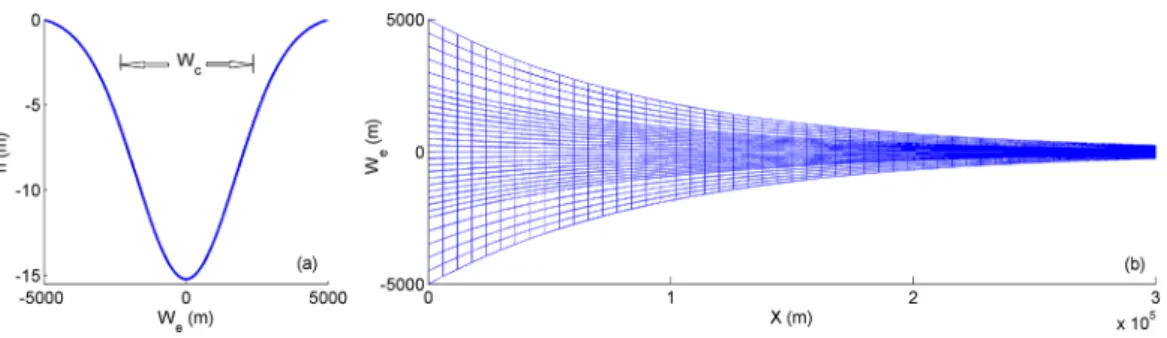
After validating MTDE using the data from prototype systems, an idealized, depth-integrated numerical 2D tidal-river model was developed using the open-source numerical model Delft3D Flow [Booij et al., 1999] to determine how measured variations in river flow, friction and other factors altering tidal properties affect discharge estimates based on MTDE. Grid properties such as the lateral depth profiles and the convergence of channel cross section in the along-channel direction are adjustable between runs and are specified para-metrically. An example of the idealized bathymetry and numerical grid is shown in Figure 5.
Our numerical model is prototype-inspired and the initial hydrodynamic/morphologic characteristics were compatible with the Columbia River system. However, later we will show that the MDTE method is applica-ble to a large non-dimensional parameter space, and hence to a variety of estuarine systems. The width of the Columbia River estuary decreases almost exponentially in the lower estuary (e.g., fromRKM 30 to RKM 140), as observed in many estuaries and often assumed in idealized estuary models [Jay, 1991;Friedrichs and Aubrey, 1994;Talke et al., 2009;Chernetsky et al., 2010;Cai et al., 2014]. However, the landward90 km of the Columbia River estuary (i.e., landward of RKM 140) is relatively constant in width, in part due to dredging and modification of the banks. The tide that reaches the Bonneville Dam at RKM 234 during low flow periods is very small [Jay et al, 2015] such that there is effectively no reflection. The dominant tidal pro-cess affecting water levels landward of RKM 170 is daily hydropower management (‘‘power peaking’’), but since this does not much affect the D2wave property [Jay et al., 2014] it is not modeled here. To eliminate
reflections in the numerical model, we have extended the numerical grid to RKM 300. The model exponen-tially converges between the mouth and RKM 200, and is straight (e.g., with constant width) between RKMs 200 and 300. Each channel cross section is Gaussian (e.g., as inHuijts et al. [2006]) and is flanked by an inter-tidal area with a constant slope (Figure 5). Smooth grid lines for any assumed convergence rate are pro-duced parametrically, such that the channel cross section contains 50 grid partitions and the intertidal areas contain 40. The estuary is divided into 750 along-channel cells. The automatic Delft3D ‘‘orthogonalization’’ software is used, and the grid is checked to ensure smoothness. The parameters that describe the bathyme-try are lengthl, channel depthH, channel widthWc, total widthWe, convergence length scaleLb. Here, the parametersH515m,l5300km, and the ratioWc/We50.5 are held constant along-channel withWe510 km at the mouth. We have used three different values of convergence length scales for the lower reach of the estuary to test the effects of geometry (Table 1). The ratio of tidal flow to river flow and the strength of bed friction are also varied systematically (three values of each), as described below.
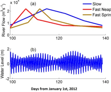
The model is forced by a time-varying river flowQRat the landward end and by theK1,O1,N2,M2andS2 tidal constituents at the seaward boundary (supporting information Table S2). Overtides are considered negligible at the seaward boundary; an appropriate assumption in both the Columbia River and Fraser River systems. Also, given that salinity intrusion is absent much of the year upstream of the two reference gauges in both prototype systems, a vertically integrated approach appropriately describes the tidal dynamics of the system. A spatially constant bottom friction coefficient is used in each scenario (Table 1). It takes24
hours for the model to adjust for start-up. To allow start-up time and include the neap-spring and K1/M2cycles, we run the model for 40 days.
We represent diverse estuarine proper-ties by altering three non-dimensional master variables that control tidal propagation through the grid described above; an example is shown in Figure 5. Thus, each new combina-tion of master variables (Table 1) yields a new scenario. While addicombina-tional variables could be added, these three were chosen based on previous idealized studies [e.g., Ianniello, 1979; Jay, 1991; Lanzoni and Seminara, 1998] to produce the smallest parameter space sufficient to realistically test MTDE. Our choices for non-dimensional variables are:
1. Friction, parameterized asw5CdLbg=H2(the inverse of the Strouhal number), whereCdis bottom fric-tion,Lbis the convergence length scale,gis the tidal amplitude andHis the total depth, for unstrati-fied flow [Ianniello, 1979]. Parameterwrepresents the effect of change in bed friction (e.g., change in bed material or bedforms), but also reflects the effect of mean sea level variability or channel deepen-ing (viaH).
2. River Discharge, parameterized asX5UR=UT(the ratio of freshwater velocity to tidal velocity). To compare
URandUT, and estimateX, assuming a constant cross-sectional area over a tidal cycle, we compare the peak river flow to the cross-sectionally averaged peak tidal discharge at the mouth. The flow might occur on different time scales ranging from days (e.g., storm-driven freshets) to months (e.g., snowmelt-driven freshets). For each magnitude ofXwe develop two hydrographs that have the same peak flows but dif-fer in the time-scale of the high-flow event (Figure 6). ‘‘Slow’’ freshets occur over a time scale of30days and ‘‘fast’’ floods occur over10days. The slow hydrographs are long enough to cover a considerable range of tidal variability. To study the sensitivity of model to spring-neap tidal effects we run the fast flood cases under two different scenarios, with the peak flow occurring during neap, and spring tides, respectively (Figure 6).
3. Convergence length scale (xLb/coLb/k), wherex,co5(gh) 1/2
andkdenote the tidal frequency, inviscid wave celerity, and inviscid tidal wavelength, respectively. By varyingLband keeping depth and wave celerity constant, we study the effect of funneling on tide propagation and the applicability of MTDE. The nondimensional variables and their range of values are presented in Table 1. Using three different values forLb,wandX, each with three subscenarios of different river flow hydrographs, produces 33333
33581 model runs in total. For each scenario we analyze water level at seven locations along the channel (at RKM 29, 53, 68, 87, 107, 138, and 172). The choice of these locations in the idealized model is compatible with the gauges located in the lower Columbia River. Next, using the approach described in section 3.2.2, we analyze the tide data to obtain the amplitude of tidal species at each station. To allow start-up time we neglect the modeled data for the first day. The resulting |C2| values were
then analyzed versus freshwater dis-charge to determine how tidal prop-erties vary with flow, using (3). The parameters in equation (3) were determined by nonlinear regression analysis for each RKM, as for the observed time series.
Table 1.Nondimensional Master Variables Used in Modeling, and Their Ranges
Variable Value 1 Value 2 Value 3
Convergence length-scale (Lb/k) 1.5 2.2 3
River flow/tidal flowX5UR/UT 0.3 0.6 0.9
Frictionw5(CdLbg/H2) 1 2 5
Figure 6.Numerical model boundary conditions for three different scenarios of gradually varying high flow event (e.g., ‘‘slow’’ freshet and ‘‘fast’’ floods): (a) river flow at the upstream boundary; (b) measured water-level at the ocean boundary.
4. Results and Discussion
4.1. Prototype SystemsRiver flow estimates for the Fraser River are compared against measurements over the 2010–2012 period (Figure 7), and show overall good agreement. We use the Nash-Sutcliffe efficiency coefficient (NSEC) [Nash and Sutcliffe, 1970] to judge the success of the estimates. For low to moderate river flow periods (<6000 m3s21), the D2 admittance amplitude |C2| located at Mission (RKM 82) best describes the variation
in river flow (Figure 7c), with an NSCE of 0.93. However, this gauge is located furthest upstream, so it could not accurately estimate flows greater than 6,000 m3s21because tidal amplitudes become negligible (Figure 7d). Further downstream, New Westminster and Port Mann, with NSEC equal to 0.87 and 0.89 respectively, work relatively well in estimating discharge over a wide range of flow rates; however both somewhat under-estimate low flows (Figures 7a and 7b). Port Mann more successfully under-estimated high flows than New Westminster.
The likely reasons that Multiple-gauge Tidal Discharge Estimate (MTDE) works well in the Fraser River are that: i) local inertia effects are negligible in strongly dissipative and weakly convergent, river-flow domi-nated systems [Lanzoni and Seminara, 1998], such that river-flow induced friction rather than constituent interactions are the primary factor affecting tidal properties; and ii) there is a large dynamic range in flow, because freshwater flows to the lower Fraser River are essentially unregulated and vary seasonally from
600 m3s21to nearly 12,000 m3s21.
Figure 8 compares measured freshwater discharge and MTDE-based discharge in the Lower Columbia Estu-ary at 6 gauges (at RKM 53, 68, 87, 107, 138, and 172) over the 2010–2012 validation period. The results sug-gest that the gauges farthest from the mouth perform best for both low and moderately high flow periods; thus, the NSEC increases monotonically in the landward direction from RKM 54 (0.32) to RKM 68 (0.67), RKM 87 (0.79), RKM 107 (0.82), RKM 138 (0.92), and RKM 172 (0.93), respectively (Figure 8). The likely reasons for this pattern is the large tidal flows, which are the same order of magnitude as river flows [Jay et al., 1990]. For example, tidal processes such as the generation of overtides and tidal monthly fluctuations dominate seaward of RKM 135, while beyond this point overtides and tidal monthly fluctuations decrease [Jay et al., 2014], and direct tidal damping by river flow is the main nonlinear interaction. Moreover, MTDE performs best at a given gauge when flow-driven D2 fluctuations in admittance are large relative to the correspond-ing neap-sprcorrespond-ing variations. Just as in the Fraser River, the best-performcorrespond-ing gauges in Columbia River are far-ther seaward for the highest flows. At the upstream gauges, resolution and precision decreases during high flow conditions due to weak tides, and the Beaver tide gauge at RKM 87 agrees better with the USGS dis-charge estimate (from a horizontal ADCP record) at the high flow event in 2011, during which it performs better than the more landward gauges.
Figure 7.Fraser River validation; (a) New Westminster (RKM 40; NSEC50.87), (b) Port Mann (RKM 45; NSEC50.89), (c) Mission (RKM 82; NSEC50.59). The observed water level at the reference gauge (Steveston) is not available from June to December 2011, so MTDE could not be used during this period.
While flows in the Columbia River are regulated so that they rarely exceed 15,000 m3s21, flows of 20,000 to 30,000 m3s21have occurred during brief winter floods on several occasions since 1964. We evaluate MTDE’s applicability to rare high flows, by estimating flows during the last such event in February 1996, which was measured only by the gauges at Astoria and Beaver. As usual, we use Astoria as the reference gauge. To show the effect of the dynamic range of the flow data used for calibration on the accuracy of flow estima-tions, we use two calibration data sets. For ‘‘Calibration A’’ (Figure 9) we calibrate MTDE with data from 2003 to 2010. For ‘‘Calibration B’’ we use all data from 2003 to 2013, including the high flow event of
15,000 m3/s from 2011, and also the data from January to March 1996, a period that includes the highest river discharge event during the last 40 years. Figure 9 compares the estimated river flow under these two calibration scenarios to measured discharge during winter 1996. With ‘‘Calibration A,’’ MTDE substantially underestimated (by20%) the peak in February 1996. This might be due to the limited dynamic range of flow during the period used for calibration (2003–2010), the limited tidal amplitude for high flows at Beaver in 1996, or the fact that the 1996 freshet was very short (only a few days) with rapid changes in flow, a situa-tion that causes difficulties for MTDE (below). The estimates under the ‘‘Calibrasitua-tion B’’ scenario, which underestimated the peak by8%, improves upon ‘‘Calibration A’’ scenario, and shows the importance of including a large dynamic range of flows during MTDE calibration. We note also that the USGS flow esti-mates used for comparison in Figure 9 are not based on gauging at Beaver. The Beaver gauging system was out of commission for the period in question, and USGS flow estimates are routed from observations at more landward locations. Thus, the USGS flow estimates are more uncertain than usual, and calibration A & B can be interpreted as independent, possibly more accurate estimates. Reasons for the relative success of the various gauges will be discussed in terms of non-dimensional parameters, below.
4.2. Physical Interpretations
The results in Figures 7–9 validate MTDE over a wide range of flow regimes in two different river estuaries, though the results suggest that there is a trade-off between optimal gauge location and river flow. Stations farther from the mouth are more sensitive to variations in river flow, and change in river flow dominates over other factors contributing to tidal wave adjustment (e.g., tidal constituent interaction). But a station too far from the mouth (e.g., relative to the horizontal length scale of tide wave propagation) will not have an observable tide during periods of very high discharge. Figure 10a conceptually depicts the along-channel variation of tidal amplitude during low and high flow events. The change in tidal amplitude due to
Figure 8.Columbia River validation; (a) Skamokawa (RKM 53; NSEC50.32), (b) Wauna (RKM 68; NSEC50.67), (c) Beaver (RKM 87; NSEC50.79), (d) Longview (RKM 107; NSEC50.82), (e) St Helens (RKM 138; NSEC50.92), and (f) Vancouver (RKM 172; NSEC50.93).
variation in river flow is small at the gauges located close to the mouth. Thus, during low-flow periods the strongest variations in admittance occur in the landward half of the system (e.g.,x/l>0.5; wherexis along-channel distance from the mouth andLis the total length of the estuary). During high-discharge periods, in contrast, variations in admittance are larger close to the mouth (forx/l<0.5), and the tide loses most of its energy before reaching the upriver gauges. Note also that spring tides damp faster than neap tides in river influenced estuaries [Jay et al., 1990;Guo et al., 2015], such that the rate of along-channel variation in admit-tance is different between spring and neap tides, even if flow is constant. Figure 10b shows the along chan-nel variation of D2amplitude during low and high flow periods for both the Columbia River and Fraser
River. A decrease in freshwater discharge in Columbia River from high flows in May 2011 (15,000 m3s21) to low flows (4000 m3s21) in December 2011 causes the D2amplitude near the mouth (x/l0.16) to rise
only by9%. In contrast, the same change in river flow causes the D2amplitude at St Helens (x/l0.58) to
increase from 0.19m to 1.25m (6.53 rise). Similarly, an increase in river flow in the Fraser River from 1000 m3s21in February 2012 up to 11,500 m3s21in June 2012 causes the D2amplitude to decrease by
10% at the mouth; while the same increase in river flow rate cause the D2amplitude at Mission (x/l0.85)
to decrease from 1.65m to 0.1m.
These results can be interpreted as follows. In the lower reaches of an estuary where cross-sectional area is large and river flow velocity is relatively small compared to tidal velocity, changes in river flow have only a limited influence on tidal properties relative to overtide generation and neap-spring adjustments caused by tidal constituent interactions. In systems in which salinity intrusion is present at the reference stations, neap-spring changes in density stratification and salinity intrusion might also influence bed friction and tidal properties. Upriver, cross-sectional area is smaller, salinity intrusion is not present, flow is uni-directional, and tidal-fluvial frictional interactions are the primary factors that modulate tides. However, under some circumstances (e.g., extremely high flow events when tidal waves are weak far upstream) a downstream gauge works better than upstream gauges, because the tide is nearly extinguished upriver and also the zone of river dominance has been moved downstream. Figure 10 shows how the D2amplitude
at Mission (Fraser River) and Vancouver (in Columbia River) tends to zero at upriver stations during extreme high-flow events. Thus, the analyses of tides in the prototype systems suggest that MTDE, in estuaries with
Figure 9.(a) scatter plot of estimated discharge versus observed discharge; and (b) time-series of estimated flow during a rare high flow event in CR (January–March 1996); For Calibration A the model is only calibrated to the data from 2003 to 2010, while for Calibration B the model is calibrated using data from 2003 to 2013 and data observed in Winter 1996.
Figure 10.(a) conceptual along-channel variation of tidal amplitude; (b) variation of the D2tidal amplitude along-channel for Fraser River (FR) low flow in February 2012 (1000 m3s21);
and FR high flow (11,500 m3
s21
) in June 2012; Columbia River (CR) low flow (4000 m3
s21
) in December 2011; and CR high flow in May 2011 (15,000 m3
s21
). Where ‘‘x’’ is the distance from the mouth and ‘‘L’’ is the total length of the estuarine tidal intrusion.
high variability in river flow, is best implemented with at least three gauges: one reference gauge near the ocean, and two other gauges strategically located along the tidal-river in a manner that corresponds well to the discharge regime of the system.
We also compare MTDE to Tidal Discharge Estimate (TDE) [Moftakhari et al., 2013] results in the Columbia River system to evaluate the improvements associated with MTDE versus TDE. For this purpose we first aver-age MTDE over 18 days (the time scale of TDE) at Vancouver for low to moderate discharge rates (e.g.,
10,000 m3s21) and at Beaver for high flow events (e.g., >10,000 m3s21). This combined MTDE is com-pared to the estimates from TDE. The 18day averaged flow is estimated via TDE using the tides observed at Astoria. Figure 11 shows the calibration curve for TDE. The separate nonlinear fits that describe the variation of M2admittance with changed discharge during low and high flow events (shown in Figure 11) are used
to estimate discharge from 2010 to 2012. Figure 12a shows the scatter plot of estimated MTDE versus the observed 3day averaged flow, Figure 12b compares the estimated TDE with the 18day averaged observed flow; and Figure 12c shows time series of observed and estimated discharges. MTDE (NSEC of 0.94) esti-mates flows during both high and low-flow periods more accurately than TDE (NSEC of 0.76).
We also compare the MTDE method against a modified version of the traditional rating curve approach in whichQRis estimated from daily mean water levels. To minimize the effect of oceanic (non-fluvial) varia-tions in average water level, we take the difference between water levels at two gauges and obtain the fol-lowing ‘‘rating curve’’ equation:
QR5a01b0ðH2HrefÞc
0
(5) wherea0,b0, andc0are coefficients, andHandHref denote the 3 day averaged water level (approximately
the same time-resolution as MTDE method) at an upstream gauge and a reference gauge, respectively.
Figure 11.TDE calibration curve for tides observed at Astoria, 2002–2009.
Figure 12.Comparison of TDE and MTDE results; (a) MTDE results versus 3 day averaged observed flow; (b) TDE results versus 18 day aver-aged observed flow; and (c) time series of the observed and estimated flows.
Figures 13a and 13b show the calibration curve of Columbia River discharge versusDh5H2Href, calculated
usingH5Wauna (13a),H5Vancouver (13b), andHref5Astoria over the years 2003–2010. Figures 13c–13e compare the estimated river flow viaDhto the observed flow 2010–2013. The results suggest this rating curve approach works reasonably well under a wide range of flows, with NSEC values of 0.83 and 0.94 for Wauna and Vancouver, respectively. This approach still has, however, limitations compared to MTDE. Far upstream it performs as well as MTDE (e.g., at Vancouver in the Columbia River), but it does not account for neap-spring storage effects that are prominent during low to medium flow periods [Jay et al., 2015], and are not captured by the reference station. As a result, Figure 13a suggests that for a flow rate of 5000 m3s21,Dhat Wauna might vary between20.42 and 0m. Thus,Dhin this range of river flow is mostly affected by factors other than discharge (e.g., by tidal range, local variability in wind setup and atmospheric pressure). Since the rating curve approach is often used to estimate discharge when direct measurements fail (as occurred for 200 days in 1997 at Beaver (Figure 1c); J. Parham (personal communication, 2014), USGS), improving upon this method can have immediate applications.
The Fraser River and Columbia River have highly variable flows and somewhat different geometries, but still cover only a limited parameter range with respect to river estuaries in general. Therefore, we evaluate in the next section the effect of variation in physical parameters and tidal characteristics on the applicability of MTDE through numerical modeling of a broad spectrum of idealized estuarine systems.
4.3. Analysis of Idealized Systems 4.3.1. Applicability of MTDE
Idealized model results illustrate (Figure 14) the behavior of MTDE in terms of contours of NSEC for the 81 hydrologic/morphologic scenarios described in section 3.5. In Figure 14, groups of three columns show the results for the three flow scenarios: slow freshet, fast flood during a neap tide, and fast flood during a spring
Figure 13.Mean slope discharge estimation approach results for CR; (a and b) calibration curves for water levels observed at Wauna and Vancouver, respectively, relative to Astoria; (c–e) estimated discharge using tides observed at Wauna and Vancouver versus 3 day averaged observed flow 2010–2012.
tide, respectively; and the first, second and third rows display results for non-dimensional convergence val-ues ofLb/k51.5, 2.2 and 3, respectively. As the results suggest, the time scale of the high flow event (e.g., gradually varying hydrographs versus rapid varying flows) affects the effectiveness of MTDE for any given set of non-dimensional numbers. Flow variations with a time scale similar to the 73hr continuous wavelet fil-ter length introduce non-stationarity into tidal behavior that cannot be completely resolved; hence, MTDE is more successful for a slow freshet than for quick-pulse floods. Any lag between the flow forcing and the tidal response might also introduce error into MTDE estimates for the ‘‘fast’’ scenarios; however, sinceJay et al. [2014] found the time lag to be less than 12 hours for the Columbia River, this is not likely an issue. The contour plots of Figure 14 help us determine the range of non-dimensional parameter space over which MTDE gives good estimations. The Columbia River and Fraser River systems are characterized as strongly convergent and weakly convergent tidal rivers, respectively [Lanzoni and Seminara, 1998], with the non-dimensional friction number being about half as large in the Columbia (WCR5CdHL2bg1:5) [Kukulka and
Jay, 2003b;Jay et al., 2011] as in the FraserWFR5CdHL2bg3:0 [MacDonald and Geyer, 2004;Kustaschuk and
Best, 2005]. High flow events occur in the Columbia River on both the fast (winter rain-on-snow events) and slow (spring snowmelt freshets) times scales [Jay and Naik, 2011] (Figures 14a–14i). Given Columbia River geometry (with nondimensional convergence ofLbk211:1) and a fast time-scale event, the model
sug-gests that MTDE should be able to successfully estimate (NSEC>0.8) low (X0.3) and moderate discharges (X0.6) using the observed tides at gauges located forx/l>0.7 and 0.4, respectively. However, for high-flow periods (X0.9), gauges located at 0.3<x/l<0.7 would be the best choices for MTDE. Because the tidal wave is weak beyondx/l0.7 during extremely high flow events, gauges beyond this point are less success-ful in estimating river flow. The modeling results are consistent with in-situ results (e.g., Figure 8), and the analysis shows that estimates at upstream locations work well, except during larger flow events (e.g., spring 2011) when gauges located in mid-estuary (x/l0.5) work best.
Model results (Figures 14j–14l) suggest that during low to moderate flow periods (X50.3 – 0.6) in a system like Fraser River (with non-dimensional convergence ofLbk212:2 andW3), MTDE best describes the
variation in river flow based on observed tide at gauges located far from the mouth. However, in Fraser, in which snowmelt freshets [Milliman, 1980;Kustaschuk and Best, 2005] cause moderate to high flow events at a monthly time-scale, high friction nearly extinguishes the tide at landward stations during high flows (X
0.9), and more seaward stations (e.g., 0.2<x/l<0.4) should be used for MTDE.
In summary, the range of non-dimensional numbers used in our numerical modeling provides a tool to describe the hydrodynamic characteristics of a variety of prototype systems (i.e., Delaware, Hudson, Poto-mac, Rotterdam Waterway and Outer Bay of Fundy [Lanzoni and Seminara, 1998]). Figure 14 provides an
Figure 14.Idealized numerical modeling results; color bar shows the Nash-Sutcliffe efficiency coefficient. The green lines indicate the locations of the Columbia (CR) and Fraser (FR) Riv-ers in the parameter space.
overview that describes conditions under which MTDE is able to accurately estimate river flow in a given system with certain hydrologic and morphologic characteristics.
4.3.2. Interpretation
Numerical model results (Figure 15; explained below) confirm the in-situ observation that MTDE discharge estimates are associated with considerable uncertainty when based on tide gauges located near the mouth of the estuary. The likely reason is that the river flow velocity is relatively small at these points (compared to tidal currents) and tidal properties at such gauges are affected by factors other than river flow velocity, especially constituent interactions (Figures 4a–4c). The Eulerian Stokes drift compensation outflow can be a sizable fraction of the total outflow during low-flow periods [Guo et al., 2015], producing error in flow esti-mates using tides observed close to the mouth. The presence and strength of Stokes drift depends on the phase difference between vertical and horizontal tides [Guo et al., 2015] and is determined by the relative importance of convergence and friction [Jay, 1991]. To the first order, the Stokes drift transport in one dimension is [Longuet-Higgins, 1969]:
Qst
1
2UTfTCosðdÞ (6)
whereQst, UT,nTandddenote the Lagrangian Stokes drift (which must be compensated by an Eulerian return flow), tidal velocity amplitude, tidal height amplitude, and the phase difference between the tidal velocity and wave amplitude, respectively. Figures 15a and 15b show the along-channel variation of the ratio between Stokes drift flow and the freshwater inflow during low and high flow periods, respectively, for an idealized tidal-river withW2. The Eulerian Stokes drift compensation flow represents an addition to the net outflow that is not part of the river discharge measurement, and which varies over the tidal month, approximately with the square of the tidal amplitude. The existence of the Stokes drift is one reason that the neap-spring term in equation (3) is needed. As the Figure 15 suggests, the Stokes drift is strongest in the lower reach of the system (e.g.,x/l<0.4), while far from the mouth it tends to zero. For high flows, model results suggest that it never exceeds6% of the river discharge and should not have a large effect on MTDE estimates. During low-discharge periods, the Stokes drift compensation flow is modeled to be up to 35% of the river discharge (Figure 15). The competing effects of river flow and Stokes drift are, accordingly, one of the reasons that MTDE is less successful during low flow periods using tides observed in the lower estuary. Nonetheless, numerical modeling results and Figures 7 and 8 suggest that MTDE can be used dur-ing low-discharge periods, if the gauge employed is properly located and calibrated.
Results for both the modeled and in-situ rivers suggest that the time scale over which a flow event occurs (i.e., gradually varying versus rapid varying flows) affects the applicability of MTDE for a given system. A pos-sible reason is the barotropic adjustment time-lag between a change in flow and the tidal response thereto; however, this lag is typically a few hours to a few days depending on the characteristics of the system. Time-varying salinity intrusion and stratification may also alter tidal properties and impact MTDE estimates, and baroclinic adjustment can be slow relative to both the tidal month and to typical time-scales of flow variations [MacCready, 1999]. For the systems analyzed here, baroclinic adjustment should not compromise
Figure 15.Along-channel variation in stokes drift flow compensation in an idealized tidal-river withW2; (a) during a low flow period, and (b) during a high flow event.QstandQdenote the Stokes drift flow compensation, and freshwater inflow to the estuary, respectively.
MTDE estimates, because all gauges are upstream of salinity intrusion, except for the reference gauges dur-ing low-flow periods.
Once calibrated, MTDE could be used as a routine flow monitoring system. Indeed, the difficulty of monitor-ing flows through the lower reaches of a tidal river, noted above, is one reason for developmonitor-ing the method. Actual implementation of such an approach would require calibration efforts beyond those discussed here, because we have not attempted to take into account flows entering the system below the last river gauge. In the Columbia River, this is only about 3% of the total average flow to the ocean, but it is about 28% in the Fraser River.
Finally, we attempted to estimate discharge in our idealized Delft3D model using the approach proposed byCai et al. [2014]. Our results suggest that this approach cannot, without modification, be applied to sys-tems with mixed diurnal/semidiurnal tides, a factor that violates one of the assumptions on which the model is based. Thus, our lack of success is consistent with expectations.
5. Conclusion
This study demonstrates the feasibility of the MTDE method for estimating freshwater inflow to river-estuaries and the ocean using tidal observations made at multiple locations along the system. By using con-tinuous wavelet transform for tidal analyses we improved the time resolution of estimates from 18 days (TDE method) [Moftakhari et al., 2013] to less than a week (MTDE). Results from two systems show that MTDE successfully estimates discharge in a variety of hydrologic regimes and can accurately/efficiently esti-mate freshwater throughout an estuary, in some cases better than previous approaches/methods (e.g., TDE, and an adjusted rating curve approach). Flow estimates based on de-tiding [Pagendam and Percival, 2015;
Lim and Lye, 2004] have not been applied widely enough to know whether they can provide comparable results.
During low to moderate-flow periods, MTDE usually works best some distance upriver from the estuary mouth, where there is a balance between cross-sectional funneling and damping of the tide by friction. However, the tide may not reach these upriver stations with sufficient amplitude during high-flow periods to allow MTDE to accurately estimate flow. During high-flow periods, MTDE based on gauges closer to the upstream limits of salinity intrusion is more effective. This suggests that practical use of MTDE in estuaries with high variability in river flow will require at least three tide gauges, a reference gauge near the ocean and two gauges further upriver.
The distribution of the Nash-Sutcliffe efficiency coefficient in the Delft3D results provides an overview of the response of the MTDE method to variations in three non-dimensional numbers and identifies the ranges for which MTDE best estimates river discharge. Numerical model runs suggest that MTDE is most effective using gauges where there is strong variability in tidal properties with flow. Close to the estuary entrance, tidal admittance variations (at least in the Columbia River and Fraser River) are small, and the tidal variability induced by fluctuating river discharge may be masked by the influences of coastal processes. Far upriver, the tides are always small, and again the range of tidal surface water level fluctuations is too small to allow accurate discharge estimates from tidal properties, especially for high flows. A convergent estuary will, it appears from numerical model results, likely exhibit a ‘‘sweet spot’’ that maximizes the variability of tides with flow and hence the resolution of MTDE. If, however, the river discharge range is sufficiently large, a sin-gle tidal-fluvial station may not adequately cover the full range of observed river discharge, leading to a need to employ three gauges. Finally, Delft3D results suggest that the contribution of the Stokes drift com-pensation flow to the total outflow of the system may interfere with MTDE estimates during low-discharge periods, at least for gauges located near the estuary mouth.
References
Alsdorf, D. E., and D. P. Lettenmaier (2003), Tracking fresh water from space,Science,301(5639), 1491–1494, doi:10.1126/science.1089802. Booij, N., R. C. Ris, and L. H. Holthuijsen (1999), A third-generation wave model for coastal regions: 1. Model description and validation,
J. Geophys. Res.,104, 7649–7666, doi:10.1029/98JC02622.
Buschman, F. A., A. J. F. Hoitink, M. van der Vegt, and P. Hoekstra (2009), Subtidal water level variation controlled by river flow and tides,
Water Resour. Res.,45, W10420, doi:10.1029/2009WR008167.
Acknowledgments
Lynne Campo in Environment Canada (ec.gc.ca) is acknowledged for sharing hourly water level data at tide gauges in Fraser River estuary. The rest of the data used in this study is readily available online (http://www.isdm-gdsi.gc.ca/); Hourly water-level data for tide gauges located in the Fraser River were downloaded from http:// wateroffice.ec.gc.ca/, the hourly water-level data for tide gauges located in the Columbia River estuary were downloaded from the National Oceanic and Atmospheric
Administration (NOAA) website (http:// tidesandcurrents.noaa.gov/), and tide data for Beaver Army Terminal were obtained from the US Geological Survey (USGS; http://or.water.usgs.gov/ ). The support for this project was provided in part by a Miller Foundation grant to the Institute of Sustainability and Systems at Portland State University and a Portland State Research enhancement grant. D.A. Jay and S.A. Talke were supported in part by the National Science Foundation (NSF) grant: Secular Changes in Pacific Tides, OCE-0929055. S.A. Talke was supported in part by two additional NSF grants: 19th Century US West Coast Sea Level and Tidal Properties, OCE-1155610 and Career: Modeling 19th-century estuaries to address 21st-century problems, award 1455350. Ramin Familkhalili is also acknowleged for his help on setting up the numerical model.