Theses & Dissertations Boston University Theses & Dissertations
2018
Bidirectional long short-term
memory network for proto-object
representation
https://hdl.handle.net/2144/31682
Thesis
BIDIRECTIONAL LONG SHORT-TERM MEMORY NETWORK FOR PROTO-OBJECT REPRESENTATION
by
QUAN ZHOU
S.B., Massachusetts Institute of Technology, 2009
Submitted in partial fulfillment of the requirements for the degree of
Master of Science 2018
© 2018 by QUAN ZHOU All rights reserved
First Reader
Dorri Poppe, Ph.D.
Principal Member Technical Staff
The Charles Stark Draper Laboratory, Inc.
Second Reader
Sang (Peter) Chin, Ph.D.
“Then Samuel took a stone and set it up between Mizpah and Shen and called its name Ebenezer; for he said, “till now the LORD has helped us”
v
ACKNOWLEDGMENTS
I would first like to thank my thesis advisor, Prof. Sang (Peter) Chin of Boston University for guidance and teaching on machine learning, compressive sensing and many other topics in computer science and mathematics. I am grateful for how much time and resources he has provided for me so that I am able to learn, expand my knowledge and think independently beyond what is learned in class.
I also would like to thank Dr. Dorri Poppe in the System Engineering division at Draper. For the past a year or so, she has trained me to be a researcher rather than a mere programmer. Without her passionate counseling and input, this thesis could not have been successfully completed. I also thank Dr Sheila Hemami for giving me the opportunity to do research under Dr Poppe. She along with Martha helped me with many logistics so that I could start and finish this thesis in time.
I express my gratitude to my parents and my brothers at Antioch Baptist Church as well. I could finish without their support over the two-year master’s program.
Finally, I want to thank God who carried me over the graduate studies and this thesis work is his doing, I merely find it out after He led me to it.
vi
QUAN ZHOU
ABSTRACT
Researchers have developed many visual saliency models in order to advance the technology in computer vision. Neural networks, Convolution Neural Networks (CNNs) in particular, have successfully differentiate objects in images through feature extraction. Meanwhile, Cummings et al. has proposed a proto-object image saliency (POIS) model that shows perceptual objects or shapes can be modelled through the bottom-up saliency algorithm. Inspired from their work, this research is aimed to explore the imbedding features in the proto-object representations and utilizing artificial neural networks (ANN) to capture and predict the saliency output of POIS. A combination of CNN and a
bidirectional long short-term memory (BLSTM) neural network is proposed for this saliency model as a machine learning alternative to the border ownership and grouping mechanism in POIS. As ANNs become more efficient in performing visual saliency tasks, the result of this work would extend their application in computer vision through successful implementation for proto-object based saliency.
vii
TABLE OF CONTENTS
ACKNOWLEDGMENTS ... v
ABSTRACT ... vi
TABLE OF CONTENTS ... vii
LIST OF TABLES ... x LIST OF FIGURES ... xi LIST OF ABBREVIATIONS ... xLLL GLOSSARY ... xv INTRODUCTION ... 1 VISUAL SALIENCY ... 2
Saliency and Attention ... 3
Saliency modeling versus saliency segmentation ... 3
SALIENCY ALGORITHMS... 5
Center-surround algorithms ... 5
Connection based saliency algorithms ... 6
... 7
Learning based saliency algorithms ... 7
PROTO-OBJECT REPRESENTATIONS ... 8
viii CNNs ... 11 RNNs and LSTMs ... 12 BRNNs ... 16 METHODS ... 19 Tools ... 19 Datasets ... 19
Input image datasets ... 19
GT heat maps ... 21
Data normalization ... 22
Training, Validation & Testing ... 22
Overfitting & Underfitting ... 23
Evaluation Metrics ... 24
EXPERIMENT I ... 28
Input representation and dimensionality ... 28
Model ... 28 Hyperparameters ... 28 Architecture ... 34 Design of Experiments ... 34 Training Results ... 36 EXPERIMENT II ... 37 GT heat maps ... 37 Model ... 37
ix
Architecture ... 37
Hyperparameters for Additional Layers ... 39
Training Results ... 40
Testing Results ... 42
L1 Norm of difference map ... 43
EXPERIMENT III: ... 46 Input ... 46 GT heat maps ... 46 Model ... 47 Training Results ... 48 Testing Results ... 51 EXPERIMENT IV: ... 54 Input ... 54 GT heat maps ... 54 Model ... 54 Training results ... 54 Testing results ... 55 DISCUSSIONS ... 57 CONCLUSIONS ... 60 BIBLIOGRAPHY ... 61 CURRICULUM VITAE ... 68
x
LIST OF TABLES
Table 1. List of parameters for POIS . ... 22
Table 2. List of Hyperparameters of the BLSTM architecture. ... 30
Table 3. BLSTM parameter profile for LFSD dataset ... 36
Table 4. AUC score for LFSD dataset training (without normalization & CONV layer) 36 Table 5. Hyperparameters in additional layers ... 39
Table 6. AUC score for LFSD dataset training @ learning rate of 0.001 ... 40
Table 7. F1 score for LFSD dataset testing (with normalization, a CONV & a maxpooling layer) ... 43
Table 8. BLSTM parameter profile for CAT dataset. ... 48
Table 9. Evaluation on training CAT dataset by categories ... 50
xi
LIST OF FIGURES
Figure 1. POIS model by JHU (Etienne-Cummings, 2014) ... 6
Figure 2. Center-surround model vs GBVS model (Harel J, 2007) ... 7
Figure 3. Neural network with input, weights, and output layer (R.A. Rensink, 2000) ... 9
Figure 4. Neural network input, hidden (weights, activation) and output layer ... 10
Figure 5. A schematic diagram of LeNet CNN ... 11
Figure 6. Feature maps in CNN (Lee, Grosse, Ranganath, & Ng, 2011) ... 12
Figure 8. Three gates of a single LSTM unit (Skymind, 2017) ... 15
Figure 8. A BRNN with both forward and backward hidden layers (Colah, 2015) ... 17
Figure 10. A schematic diagram of generating GT data ... 21
Figure 11. Overfitting problem in training ANNs data (Karpathy, 2017). ... 23
Figure 12. Precision, Recall and F-measure equations ... 25
Figure 13. A Schematic diagram of BLSTM Evaluation ... 27
Figure 14. A schematic diagram of generating input data ... 28
Figure 15. 4-hidden-layer BLSTM architecture ... 34
Figure 16. 7 layer CNN+BLSTM architecture ... 40
Figure 17. Saliency prediction output vs GT in a 4-layer BLSTM architecture ... 41
Figure 18. PR & ROC curve of a trained CNN+BLSTM saliency network ... 41
Figure 19. Testing sample of CNN+BLSTM saliency network ... 42
Figure 20. ROC curve for CNN+BLSTM saliency network testing on 20 LFSD images 43 Figure 21. Testing sample of CNN+BLSTM saliency network ... 44
xii
Figure 22. Improving performance of ANNs with increasing training data (Szolovitz,
2016) ... 44
Figure 23. PR curve for CNN+BLSTM saliency network training >1600 CAT images . 49 Figure 24. ROC curve for CNN+BLSTM network training CAT images by categories . 50 Figure 25. Examples of noisy training input and groundtruth labels ... 51
Figure 26. Testing samples of CAT dataset using CNN+BLSTM model ... 52
Figure 27. ROC curve for CNN+BLSTM network on testing samples of CAT dataset . 52 Figure 28. Output of CNN+BLSTM model for grayscale (no color channel) images ... 53
Figure 29. ROC and PR curves for NUSEF training data ... 55
Figure 30. ROC and PR curves for NUSEF data (both trainng and testing set) ... 56
xiii
AUC ... area under the curve AWS ... adaptive whitening saliency BLSTM ... bidirectional long short-term memory network BO ... border ownership BPTT ... backpropagation Through Time BRNN ... bidirectional recurrent neural network BS ... batch size BU ... bottom-up approach CC ... correlation coefficient CNN ... convolutional neural network DNN ... deep neural network DR ... dropout rate FP ... false positives FPR ... false positive rate G cells ... grouping cells GBVS ... graph based visual saliency HLS ... hidden layer size IAPS ... international affective picture system JHU ... Johns Hopkins University LFSD ... light field saliency dataset
xiv
MLP ... multi-layer perceptron network NLL ... negative log likelihood NLP ... natural language processing NUS ... National University of Singapore PCA ... principal component analysis POIS ... proto-object image saliency model ReLU ... rectified linear unit RNN ... recurrent neural network ROC ... receiver operating characteristic curve SGD ... stochastic gradient descent TD ... top-down approach TP ... true positives TPR ... true positive rate
xv
GLOSSARY
(The following glossary is excerpt from http://www.wildml.com/deep-learning-glossary/)
Activation Function
To allow Neural Networks to learn complex decision boundaries, we apply a nonlinear activation function to some of its layers. Commonly used functions include sigmoid, tanh, ReLU (Rectified Linear Unit) and variants of these.
Adadelta
Adadelta is a gradient descent based learning algorithm that adapts the learning rate per parameter over time. It was proposed as an improvement over Adagrad, which is more sensitive to hyperparameters and may decrease the learning rate too aggressively. Adadelta It is similar to rmsprop and can be used instead of vanilla SGD.
Adagrad
Adagrad is an adaptive learning rate algorithms that keeps track of the squared gradients over time and automatically adapts the learning rate per-parameter. It can be used instead of vanilla SGD and is particularly helpful for sparse data, where it assigns a higher learning rate to infrequently updated parameters.
Adam
Adam is an adaptive learning rate algorithm similar to rmsprop, but updates are
directly estimated using a running average of the first and second moment of the gradient and also include a bias correction term.
Alexnet
Alexnet is the name of the Convolutional Neural Network architecture that won the ILSVRC 2012 competition by a large margin and was responsible for a resurgence of interest in CNNs for Image Recognition. It consists of five convolutional layers, some of which are followed by max-pooling layers, and three fully-connected layers with a final 1000-way softmax. Alexnet was introduced in ImageNet Classification with Deep Convolutional Neural Networks.
Average-Pooling
Average-Pooling is a pooling technique used in Convolutional Neural Networks for Image Recognition. It works by sliding a window over patches of features, such as pixels,
xvi
and taking the average of all values within the window. It compresses the input representation into a lower-dimensional representation.
Backpropagation
Backpropagation is an algorithm to efficiently calculate the gradients in a Neural Network, or more generally, a feedforward computational graph. It boils down to applying the chain rule of differentiation starting from the network output and
propagating the gradients backward. The first uses of backpropagation go back to Vapnik in the 1960’s, but Learning representations by back-propagating errors is often cited as the source.
Backpropagation Through Time (BPTT)
Backpropagation Through Time (paper) is the Backpropagation algorithm applied to RNNs. BPTT can be seen as the standard backpropagation algorithm applied to an RNN, where each time step represents a layer and the parameters are shared across layers. Because an RNN shares the same parameters across all time steps, the errors at one time step must be backpropagated “through time” to all previous time steps, hence the name. When dealing with long sequences (hundreds of inputs), a truncated version of BPTT is often used to reduce the computational cost. Truncated BPTT stops backpropagating the errors after a fixed number of steps.
Bidirectional RNN
A Bidirectional Recurrent Neural Network is a type of Neural Network that contains two RNNs going into different directions. The forward RNN reads the input sequence from start to end, while the backward RNN reads it from end to start. The two RNNs are stacked on top of each other and their states are typically combined by appending the two vectors. Bidirectional RNNs are often used in Natural Language problems, where we want to take the context from both before and after a word into account before making a prediction.
Categorical Cross-Entropy Loss
The categorical cross-entropy loss is also known as the negative log likelihood. It is a popular loss function for categorization problems and measures the similarity between two probability distributions, typically the true labels and the predicted labels. It is given by L = -sum(y * log(y_prediction)) where y is the probability distribution of true labels (typically a one-hot vector) and y_prediction is the probability distribution of the predicted labels, often coming from a softmax.
xvii
Input data to Deep Learning models can have multiple channels. The canonical examples are images, which have red, green and blue color channels. An image can be represented as a 3-dimensional Tensor with the dimensions corresponding to channel, height, and width. Natural Language data can also have multiple channels, in the form of different types of embeddings for example.
Convolutional Neural Network (CNN, ConvNet)
A CNN uses convolutions to connected extract features from local regions of an input. Most CNNs contain a combination of convolutional, pooling and affine layers. CNNs have gained popularity particularly through their excellent performance on visual recognition tasks, where they have been setting the state of the art for several years.
Dropout
Dropout is a regularization technique for Neural Networks that prevents overfitting. It prevents neurons from co-adapting by randomly setting a fraction of them to 0 at each training iteration. Dropout can be interpreted in various ways, such as randomly sampling from an exponential number of different networks. Dropout layers first gained popularity through their use in CNNs, but have since been applied to other layers, including input embeddings or recurrent networks.
Embedding
An embedding maps an input representation, such as a word or sentence, into a vector. A popular type of embedding are word embeddings such as word2vec or GloVe. We can also embed sentences, paragraphs or images. For example, by mapping images and their textual descriptions into a common embedding space and minimizing the distance between them, we can match labels with images. Embeddings can be learned explicitly, such as in word2vec, or as part of a supervised task, such as Sentiment Analysis. Often, the input layer of a network is initialized with pre-trained embeddings, which are then fine-tuned to the task at hand.
Exploding Gradient Problem
The Exploding Gradient Problem is the opposite of the Vanishing Gradient Problem. In Deep Neural Networks gradients may explode during backpropagation, resulting in number overflows. A common technique to deal with exploding gradients is to perform Gradient Clipping.
Fine-Tuning
Fine-Tuning refers to the technique of initializing a network with parameters from another task (such as an unsupervised training task), and then updating these parameters
xviii
based on the task at hand. For example, NLP architecture often use pre-trained word embeddings like word2vec, and these word embeddings are then updated during training based for a specific task like Sentiment Analysis.
Gradient Clipping
Gradient Clipping is a technique to prevent exploding gradients in very deep networks, typically Recurrent Neural Networks. There exist various ways to perform gradient clipping, but the a common one is to normalize the gradients of a parameter vector when its L2 norm exceeds a certain threshold according to new gradients = gradients *
threshold / l2_norm(gradients).
LSTM
Long Short-Term Memory networks were invented to prevent the vanishing gradient problem in Recurrent Neural Networks by using a memory gating mechanism. Using LSTM units to calculate the hidden state in an RNN will help to the network to efficiently propagate gradients and learn long-range dependencies.
Max-Pooling
A pooling operations typically used in Convolutional Neural Networks. A max-pooling layer selects the maximum value from a patch of features. Just like a convolutional layer, pooling layers are parameterized by a window (patch) size and stride size. For example, we may slide a window of size 2×2 over a 10×10 feature matrix using stride size 2, selecting the max across all 4 values within each window, resulting in a new 5×5 feature matrix. Pooling layers help to reduce the dimensionality of a representation by keeping only the most salient information, and in the case of image inputs, they provide basic invariance to translation (the same maximum values will be selected even if the image is shifted by a few pixels). Pooling layers are typically inserted between successive
convolutional layers.
MNIST
The MNIST data set is the perhaps most commonly used Image Recognition dataset. It consists of 60,000 training and 10,000 test examples of handwritten digits. Each image is 28×28 pixels large. State of the art models typically achieve accuracies of 99.5% or higher on the test set.
Momentum
Momentum is an extension to the Gradient Descent Algorithm that accelerates or damps the parameter updates. In practice, including a momentum term in the gradient descent updates leads to better convergence rates in Deep Networks.
xix
Multilayer Perceptron (MLP)
A Multilayer Perceptron is a Feedforward Neural Network with multiple fully-connected layers that use nonlinear activation functions to deal with data which is not linearly separable. An MLP is the most basic form of a multilayer Neural Network, or a deep Neural Networks if it has more than 2 layers.
Recurrent Neural Network (RNN)
A RNN models sequential interactions through a hidden state, or memory. It can take up to N inputs and produce up to N outputs. For example, an input sequence may be a sentence with the outputs being the part-of-speech tag for each word (N-to-N). An input could be a sentence, and the output a sentiment classification of the sentence (N-to-1). An input could be a single image, and the output could be a sequence of words corresponding to the description of an image (1-to-N). At each time step, an RNN calculates a new hidden state (“memory”) based on the current input and the previous hidden state. The “recurrent” stems from the facts that at each step the same parameters are used and the network performs the same calculations based on different inputs.
ReLU
Short for Rectified Linear Unit(s). ReLUs are often used as activation functions in Deep Neural Networks. They are defined by f(x) = max(0, x). The advantages of ReLUs over functions like tanh include that they tend to be sparse (their activation easily be set to 0), and that they suffer less from the vanishing gradient problem. ReLUs are the most commonly used activation function in Convolutional Neural Networks. There exist several variations of ReLUs, such as Leaky ReLUs, Parametric ReLU (PReLU) or a smoother softplus approximation.
RMSProp
RMSProp is a gradient-based optimization algorithm. It is similar to Adagrad, but introduces an additional decay term to counteract Adagrad’s rapid decrease in learning rate.
SGD
Stochastic Gradient Descent (Wikipedia) is a gradient-based optimization algorithm that is used to learn network parameters during the training phase. The gradients are typically calculated using the backpropagation algorithm. In practice, people use the minibatch version of SGD, where the parameter updates are performed based on a batch instead of a single example, increasing computational efficiency. Many extensions to vanilla SGD exist, including Momentum, Adagrad, rmsprop, Adadelta or Adam.
xx
Softmax
The softmax function is typically used to convert a vector of raw scores into class
probabilities at the output layer of a Neural Network used for classification. It normalizes the scores by exponentiating and dividing by a normalization constant. If we are dealing with a large number of classes, a large vocabulary in Machine Translation for example, the normalization constant is expensive to compute. There exist various alternatives to make the computation more efficient, including Hierarchical Softmax or using a sampling-based loss such as NCE.
TensorFlow
TensorFlow is an open source C++/Python software library for numerical computation using data flow graphs, particularly Deep Neural Networks. It was created by Google. In terms of design, it is most similar to Theano, and lower-level than Caffe or Keras.
Vanishing Gradient Problem
The vanishing gradient problem arises in very deep Neural Networks, typically Recurrent Neural Networks, that use activation functions whose gradients tend to be small (in the range of 0 from 1). Because these small gradients are multiplied during backpropagation, they tend to “vanish” throughout the layers, preventing the network from learning long-range dependencies. Common ways to counter this problem is to use activation functions like ReLUs that do not suffer from small gradients, or use architectures like LSTMs that explicitly combat vanishing gradients. The opposite of this problem is called the
exploding gradient problem.
VGG
VGG refers to convolutional neural network model that secured the first and second place in the 2014 ImageNet localization and classification tracks, respectively. The VGG model consist of 16–19 weight layers and uses small convolutional filters of size 3×3 and 1×1.
INTRODUCTION
Visual saliency has been widely applied to various computer vision tasks such as segmentation (Yu., 2015), image retargeting (Shamir, 2010), and object detection and recognition (Itti A. B., 2016). Many saliency models, including Hou saliency (Zhang, 2007) and Adaptive Whitening Saliency (Pardo, 2012) are based on feature extraction and normalization to transform images into saliency images for better and efficient learning result. However, in Cummings’ work (Etienne-Cummings, 2014), instead of aiming at individual features of an image, they proposed a proto-object-based algorithm that captures the perceptual organization of the whole image. In this study, a combined network of CNN and BLSTM architecture is proposed to learn and predict these proto-object representations. This research is motivated by the Gestalt attention theory and Cummings’ POIS model, and is to validate machine learning as a methodology for saliency learning.
VISUAL SALIENCY
Visual saliency or salience is generally defined as the quality by which any peculiarity stands out relative to its surrounding (Itti L. , Visual salience, 2007). Humans are born with this quality (Baluch & Itti, 2011) and able to perform tasks such as finding a set of keys to looking for a friend in a crowded place on a daily basis. For many years, it has been a subject matter in disciplines of cognitive science such as psychology, artificial intelligence, and neuroscience (Thagard, 2007). The mechanisms by which humans grant certain stimuli more attentional focus than others probably hold root in our evolutionary past. Over the past 20 years since Itti et al. research, not only saliency became a subject matter in computer vision but by these biologically-plausible mechanisms computers are able to perform object recognition and saliency detection tasks (Treisman & Gelade, 1980) (Walther & Koch, 2006) (Kienzle W, 2009) (Etienne-Cummings, 2014). The success of saliency techniques – particularly in the computer vision domain – is greatly due to their inexpensive and fast computation (i.e. various weighting schemes and optimizers used in ANNs (Krig, 2014)) . This facilitates their use as a preprocessing step in many applications. For instance, image/video compression can benefit from variable compression rate which is achieved by higher compression rate on non-salient regions and careful handling of salient area (Guo & Zhang, 2010). Saliency can provide an efficient framework for object recognition in conjunction with selective attention-based methods by underlining the informative regions (Walther & Koch, 2006). Similar idea exists in many applications that use saliency such as tracking (Itti & Borji, Exploiting local and global patch rarities for saliency detection, 2012), content-aware
image re-targeting (Jacobson N, 2010), image thumbnailing (Cifarelli, Csurka, & Marchesotti, 2009), and video summarization (Ma YF, 2005).
Saliency and Attention
In the computer vision community, there is often a confusion between attention and saliency. The two terms are used interchangeably, though there is a profound difference. Attention is a general concept that depends on many cognitive factors. It is easily influenced by the assigned task (e.g., free-viewing and interactive tasks) and the strategy of solving the task. The mechanism of attention is either expectation-driven top-down and/or scene-driven bottom-up. It is often speculated that the first is deliberative and task dependent, while the latter is reflexive and deployed by saliency (Egeth, 1997) (Baluch & Itti, 2011). However, saliency relies on the perceived visual stimulus (i.e., it is a bottom-up process) or the extracted features from the stimulus which can be
manipulated by top-down cues (Etienne-Cummings, 2014). In this thesis, the models are explored to detect saliency based on bottom-up process.
Saliency modeling versus saliency segmentation
A computer vision perspective promotes categorizing saliency studies into two main areas of debate: saliency modeling and saliency segmentation. Although the two are closely related, their objectives are distinct. The goal of saliency modeling is predicting eye movement patterns (Bruce & Tsotsos, 2006), whereas saliency segmentation is generating masks that match the annotated silhouettes of salient objects (Achanta, 2009).
While segmentation usually applies to images containing one well-identifiable object, saliency modeling is applied to and challenged by real world images with complicated scenery. Consequently, the evaluation criteria and ground truth (GT) of the two saliencies are different. Assessment of saliency segmentation is often performed by measuring the precision-recall of the output of methods against the GT data, which can be obtained from annotating the salient area by explicit judgments of observers (Pomplun, 2013). On the other hand, evaluation of saliency modeling is sophisticated and relies on observers’ eye movements. In this thesis, the methodology and evaluation of saliency learning is aligned with saliency modeling. While the focus of this research is not on how accurate it predicts the eye fixation but on the similarities and precision-recall for the prediction of proto-object representations, using machine learning.
SALIENCY ALGORITHMS
Among all saliency models and techniques in the literature, those defined by the saliency components (whether based on top-down or bottom-up process) are examined. In this section of the thesis, three types of saliency models are discussed upon which our approach and model selections are built.
Center-surround algorithms
Many saliency models rely on Feature Integration Theory (Treisman & Gelade, 1980) and feature maps (Ullman, 1985). They often consist of three steps: feature
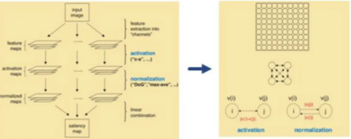
extraction, center-surround feature comparison and conspicuity map fusion. For instance, Itti et al. subsamples a given image into a Gaussian pyramid (Itti, 2005). For instance, Itti et al. subsamples a given image into a Gaussian pyramid (Itti, 2005). At each pyramid level, extracted feature channels consist of red, green, blue, yellow, intensity, and local orientations. Then, conspicuity maps are computed by comparing the value of features to the value of their surroundings features. Next, the conspicuity maps of each feature channel are combined across all scales to produce another level of conspicuity maps. Eventually, the saliency map is obtained from the linear combination of these conspicuity maps. Etienne-Cummings’ group at Johns Hopkins University (JHU) proposed a proto-object image saliency (POIS) model based on the Itti framework, and implemented border ownership (BO) cells and grouping mechanism on top of a center-surround algorithm (Figure 1). This thesis will attempt to model the input-output relationship of
POIS, and the saliency maps generated by the POIS algorithm is the source of GT data for this thesis.
Figure 1. POIS model by JHU (Etienne-Cummings, 2014)
Connection based saliency algorithms
Connection based models consider a structural relation between image pixels or regions. Saliency is modelled through the interactions of these interconnected pixels and regions. Harel et al. utilized a fully-connected graph (graph-based visual saliency, or GBVS) for salience over image locations (Figure 2), and weights between two nodes are assigned proportional to the similarity of feature values and their spatial distance (Harel J, 2007). Pang et al. presented a stochastic model that utilized dynamic Bayesian networks to predict eye fixation in a video (Pang, 2008). The model consists of deterministic
saliency maps that present the current video frame salience and stochastic saliency maps that integrate the information from the past into current video frames. These models are based on feature extraction and are complex and implementing them requires detailed parameter settings.
Learning based saliency algorithms
Learning based models establish a relation between either low-level features and eye movement statistics or the features themselves by learning classifiers, some
parameter profile, and/or some priors. Kienzle et al. fitted a non-linear support vector clustering algorithm (or SVM) to associate image patches with eye movement statistics (Kienzle W, 2009). They extracted 13x13 windows which they then transformed into 169 length feature vectors, and labelled them with a binary label denoting relation to eye fixation. Zhao & Koch implemented AdaBoost algorithm to learn the optimal weights and biases of bottom-up feature maps from observer’s eye movement data (Zhao & Koch,
2012). Moreover, advances in deep learning have driven saliency prediction to new levels of capacity and efficiency. SalNet (Junting Pan, 2016), DeepFix (Kruthiventi, Ayush, & Babu, 2017) and many other convolutional neural networks have shown deep neural
networks (ANNs) perform far better than other non-learning-based models in all evaluation metrics including AUC, F-measure, etc. Therefore, the focus of this thesis is on exploring a different ANN architecture and is aimed to study the hyperparameter domain of ANNs which is able to excel in predicting proto-object representations.
PROTO-OBJECT REPRESENTATIONS
Rensink et al. proposed a coherence theory of attention (R.A. Rensink, 2000) that prior to focused attention there is a stage of rapid processing of low-level (only the geometric and photometric properties) information across the visual field by the human eyes. The result structures, or proto-objects, are coherent over a small region of space and time. The coherence field is formed via feedback between the proto-objects and a mid-level nexus (Figure 3). The feedback in the POIS model was achieved through the interactions of border ownership (BO) cells and grouping (G) cells. Craft et al. (Craft, 2007) discovered through a recurrent learning-based network that patterns in the temporal domain (which was not investigated in POIS model) could improve and ensure more accurate BO and G assignment. Their recurrently connected network inspired BRNN architecture for this thesis work.
NEURAL NETWORKS
A neural network consists of multiple layers of interconnected artificial “neurons” that exchange information between each other (Figure 4). The connections have numeric weights that are tuned during the training process, so that a properly trained network will respond correctly when presented with an image to recognize. The advantage of the neural networks in image recognition is that they are able to learn hidden and strongly non-linear dependencies between input and output vectors.
Figure 4. Neural network input, hidden (weights, activation) and output layer
Previous research has shown convolutional neural networks have successes in visual recognition and saliency tasks. CNNs are examples of feedforward network. There is evidence that proto-object representations emerge as a natural outcome for saliency prediction (Shen, 2015). While CNNs have remarkable performance for learning-based saliency, this work seeks to demonstrate that a bidirectional recurrent neural network is able to mimic a center-surround saliency algorithm. To do this, the proto-object based saliency model will be trainedin a supervised manner, given POIS GT images as the desired outputs, with both forward and backward sequential learning.
CNNs
Convolutional neural networks are biologically-inspire variants of feed forward networks. A convolutional layer (CONV layer) mimics the simple cells of an animal’s visual cortex which respond maximally to specific edge-like patterns within their receptive field, and a max-pooling layer functions as complex cells learning the exact pattern of the larger receptive field (Hubel, 1968). Figure 5 shows a full CNN
architecture, also known as LeNet and was developed by LeCun and Bengio (Y. LeCun, 1998).
Figure 5. A schematic diagram of LeNet CNN
Through a CONV layer, the pixel matrix of an input image is transformed into a feature map, with linear filters or kernels; Each filter functions as a feature detector, and with more filters, more information about the input volume can be learned (Deshpande, 2017). After being converted to a feature map, an activation function is applied so it becomes an activation map, in which low level features are stored. A max-pooling layer then down-samples the activation map (or subsamples) spatially and uses MAX operation on each pooling filter. According to Karpathy et al., only two variations of the max pooling layer are found in practice: a pooling layer (with symbol F) of filter size of 3 and a stride (with symbol S) of 2, and more commonly F=2, S=2.
Figure 6. Feature maps in CNN (Lee, Grosse, Ranganath, & Ng, 2011)
These made up the lower layers of a CNN and a fully connected (FC) layer sums up all feature maps from the lower layers. Figure 6 illustrates the feature representations learned in both lower layers and upper layers.
In this thesis, a kernel size of 7x7 was selected to recognize proto-objects instead of the Gabor filters. The number of filters was increased (up to 64) compared to the POIS model where eight border ownership kernels responsible for mapping object activity in the pyramids were implemented (Etienne-Cummings, 2014). Like BO kernels, they are responsible for extraction of object edges and other low-level features as well. For the maxpooling layer, which mimics the grouping mechanism in POIS model, downsamples from 4 to 1 (using a pooling filter stride of 2) and the output volume of this layer will be used for the saliency detection input for the BRNN network.
RNNs and LSTMs
While a feedforward network only considers the current input to which it has been exposed, a recurrent neural network (RNN) considers both the input from the current time step and the output from the previous time step. Because RNNs ingest output from the
previous time state, they can be trained to perform tasks that feedforward networks can’t. For example, a CNN can be trained to recognize objects from the low-level features (Simonyan & Zisserman, 2015) but may not identify which object(s) are salient. Through feature extraction, a CNN can recognize patterns of the images in the spatial domain and then combine them. However, RNNs could also identify features from the time domain of input-output relationships.
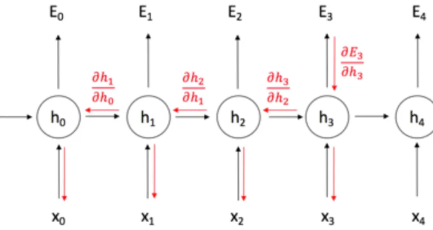
RNNs are widely applied in pattern recognition in speech data, equential text, and any other time-series data in the literature (Graves, Mohamed, & Hinton. , 2013)(Ba, Mnih, & Kavukcuoglu, 2015). Just as human memory circulates in the neurons, information circulates in the hidden states of RNNs (Mohs, 2007). This is achieved by doing a sequence of forward and backward passes through the network (Figure 7) similar to the firing of the neurons in the brain. A forward pass consists of driving the input vector and propagating the activations through to get the values of the output.
Mathematically, this can be expressed as:
ℎ" = $(&'"+ )ℎ"*+)
The hidden state at time step t is ℎ", and it is a function of the input '", modified by a weight matrix &added to the hidden state of the previous time step ℎ"*+ multiplied by its own hidden-state-to-hidden-state matrix ). It is this application of ℎ"*+ and matrix )
that puts the recurrence in RNNs. The sum of the weighted input and hidden state is squashed by the function $ – either a logistic sigmoid function or hyperbolic tangent (tanh) function, which depends on the nature of data. The activation function is able to condense very large or very small values into a logistic space, as well as make gradients workable for backpropagation.
When training an RNN, the values of the output neurons of the hidden state are compared to either the value of the next input or the desired output. The sum of the L2 error (squared error) marks the loss of the network.
A backward pass updates the weights in the network through gradient decent. The weight gradient ∇. is calculated as the derivative of the loss function with respect to the weight &". At each backward pass the weights are adjusted by multiplying this calculated gradient by the learning rate / and subtracting it from the current weight:
&"0+= &"− /∇.(&")
While RNNs have an advantage over feedforward networks for both spatial and temporal information, the gradients are susceptible to vanishing or exploding because the layers and time steps of an RNN relate to each other through multiplication. Exploding gradients can result in numerical instability thus leading a computation program to crash, whereas vanishing gradients can become too small for computers to effectively work with and thus for networks to learn.
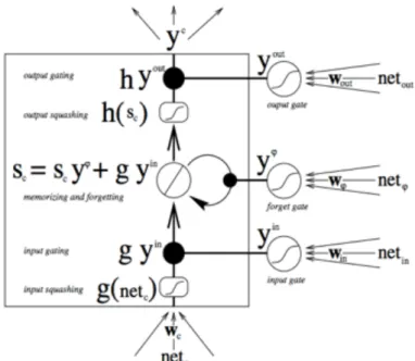
Long short-term memory networks, or LSTMs, are a class of RNN that solve both these gradient problems. LSTMs have multiple gates such that information can be stored in, written to, or “erased”. These gates act on the signals they receive and, similar to the
neural network nodes, block or pass on information by pixel-wise multiplication operation of weight matrix and input of the hidden nodes in the sigmoid layer (Rolah, 2015). The output, which is between zero and one, describes how much of each
component should be let through. Each gate has its own weight matrix (namely, Wi, Wj, Wo, Wc) and these weights, like the weights that modulate input and hidden state
connections in feed forward networks (Figure 4), are adjusted via the recurrent network’s
learning process (Figure 8). That is, the cells learn when to allow data to enter, leave or be deleted through the iterative process of making guesses, backpropagating error, and adjusting weights via gradient descent.
LSTMs have achieved good performances on several tasks including objection recognition, image and video captioning (J. Donahue, 2015) (Li & Karpathy, 2015) (Q. Wu, 2016). They could be directly employed for time dependent input, but not saliency prediction where CNNs are better for spatial features. Craft et al. studied proto-object representations and concluded that these proto-objects were closely interrelated with the boundary information in a sequential manner (Craft, 2007). Moreover, Cucciara et al. developed a saliency attentive model (SAM) combining a trained 16-layer CNN (VGG-16), which serves to extract feature maps from the input images, and one additional LSTM hidden layer for saliency map prediction (Cornia, Baraldi, Serra, & Cucchiara, 2016). They showed that a CNN network followed by LSTM sequentially enhanced saliency prediction. Their work has set precedence of implementing CNN and LSTM inspired this work that the architecture would enhance learning of the proto-object representations.
BRNNs
BRNNs are essentially two RNNs stacked on top of each other and the output is computed based on the hidden state of both RNNs (Figure 8). Since image data can be processed into sequences where information can be extracted and stored along any directions, BRNNs could propagate double the information flowing from different regions of the image. The training procedure for the unfolded bidirectional network over time can be summarized as follows.
Run all input data for one time slice through the BRNN and determine all predicted outputs.
• Do forward pass just for forward states and backward states.
• Do forward pass for output neurons.
2. BACKWARD PASS
Calculate the part of the objective function derivative for the time slice used in the forward pass.
• Do backward pass for output neurons.
• Do backward pass just for forward states and backward states.
3. UPDATE WEIGHTS
Figure 8. A BRNN with both forward and backward hidden layers (Colah, 2015)
A BRNN can be trained to perform tasks such as handwritten digit recognition (Giancarlo Zaccone, 2017), image-to-text learning (Li & Karpathy, 2015) and speech recognition (Graves, 2005). Combing BRNN with LSTM leads to a BLSTM architecture: it is just an upgrade upon BRNN that there are a forward LSTM hidden layer and a backward LSTM hidden layer, each of which functions just like a LSTM network (A. Graves, 2005). The advantage of a BLSTM architecture over a unidirectional LSTM is
that the number of hidden layers make it a deeper network, hence with more hyper-parameters the number of information from all hidden nodes increases. Additionally, because the weight matrix for forward and backward hidden sequence is separate, this enables the network to learn long term sequence-to-sequence interactions by making use of past and future context information at high level data space (Graves, Mohamed, & Hinton, 2013). Since BRNNs have achieved competitive performance to the state-of-the-art learning results on speech recognition and image captioning (Wang, Yang, Bstate-of-the-artz, & Meinel, 2016), one would expect it does the same for saliency detection. Meanwhile, this thesis work is one of the first research works implementing BLSTM on saliency maps for saliency detection tasks. Given the high performance on texts and speech data and the novelty of application, BLSTM is selected as the main type of architecture for this thesis work. Furthermore, a combined CNN+BLSTM architecture is studied and would be appealing to see if it replicates the results of hard-coded POIS model by JHU (Etienne-Cummings, 2014).
METHODS
Tools
The codes written for this thesis work are in python (2.6 and above) and matlab (2016b and above). The brnn library (Harer, 2017) was provided and modified based on the architecture of the network needed for this thesis work. The POIS model program is provided by Cummings et al. from JHU and its module is open source on their research website (CSMSL, 2017). The machine learning libraries are provided by tensorflow (version 1.0 and above) and are built on a Ubuntu 14.04.5 LTS system with 4 GPUs (two Nvidia TITAN X and two GeForce GTX) installed.
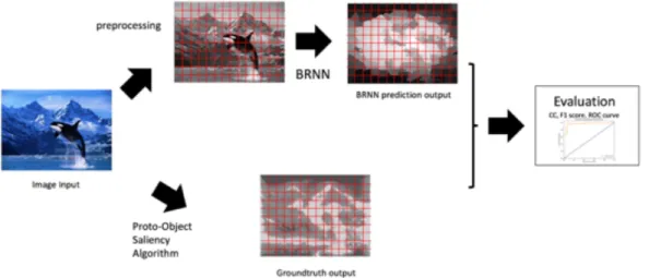
Datasets
The image datasets for this thesis work are of two types: original input images from three datasets that are converted to gray scale and used as input to the BLSTM, and the output saliency heat maps as generated by the POIS algorithm given original (non-grey scale) input images. The POIS saliency heat maps are by definition the GT to which the output of the BLSTM will be compared.
Input image datasets
• LFSD (light field saliency dataset). This dataset includes 100 one-object-focused images. This dataset is one of the benchmark datasets for saliency detection. The light field of a scene provides useful focuses, depths, and object cues. proto-objects can be
easily separated from similar or cluttered backgrounds by exploiting their light field depth (Jun Zhang, 2015) .
• CAT2000 provided by MIT Saliency Benchmark dataset (Bylinskii, 2016). This dataset contains both training and testing image set totaled 4000 images from 20 different categories: Action, Affective, Art, BlackWhite, Cartoon, Fractal, Indoor, Inverted,
Jumbled, LineDrawing, LowResolution, Noisy, Object, OutdoorManMade, OutdoorNatural, Pattern, Random, Satellite, Sketch, and Social. This is a more
challenging dataset where salient objects are not distinguished just by light field depth but by color, orientation, shapes and edges, etc. It is expected that the input-output transfer functions are dependent on these features, but not on the image categories for both the POIS algorithm and this thesis’ BLSTM.
• NUS (Nation University of Singapore) Eye Fixation dataset. This dataset contains a pool of 447 images over 75 subjects. The color images from everyday scenes from Flickr, Google Images and The International Affective Picture System(IAPS) (Doermann., 2015). An important feature of this dataset compared to the other two is that it contains many semantically affective objects/scenes such as expressive faces, interactive actions, thus providing a good source for sentiment analysis (Zhi, 2014). The training set contains 400 images and the test set 40. It is interesting to see what POIS model would regard as salient proto-objects from this dataset and whether BLSTM architecture would be able to replicate that.
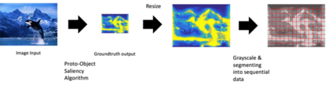
GT heat maps
GT saliency maps are generated using the POIS model provided by JHU. The input color images will undergo three stages of preprocessing, (Etienne-Cummings, 2014): feature extraction, three-channel activation (color, intensity and orientation) and normalization. The POIS output heat maps need several more processing steps to put them into a useful GT format for comparison with BLSTM output: they are resized into the same dimension as the input images (Figure 10); they are converted to grayscale and then the image matrix is segmented into sequences of equal length to be stored as prediction labels.
Figure 10. A schematic diagram of generating GT data
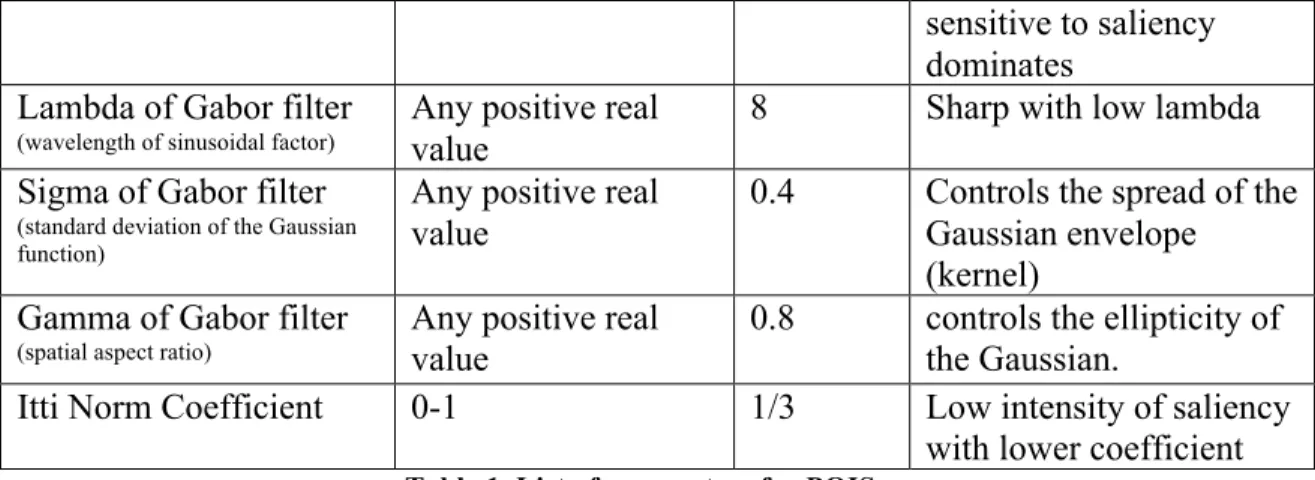
The default parameter settings for GT POIS heat maps are listed in the following table. Varying any of the parameters would result in different heat maps. In this study, the default values are fixed for all GT images.
Parameters Range Default
value
Effect
Pyramid level (M) Min=1 (fixed)
Max = 1-10 Max =10 Less specificity with larger M
downSample mode Half/full half full downsampling
produce poorer saliency Feature channels intensity (I)
color opponency (C) orientation (O)
ICO Depending on the image
sensitive to saliency dominates
Lambda of Gabor filter
(wavelength of sinusoidal factor)
Any positive real value
8 Sharp with low lambda
Sigma of Gabor filter
(standard deviation of the Gaussian function)
Any positive real value
0.4 Controls the spread of the Gaussian envelope (kernel)
Gamma of Gabor filter
(spatial aspect ratio)
Any positive real value
0.8 controls the ellipticity of the Gaussian.
Itti Norm Coefficient 0-1 1/3 Low intensity of saliency
with lower coefficient Table 1. List of parameters for POIS .
Data normalization
The input data, after converting to grayscale and segmented into sequences, were then normalized. This is mainly due to the fact that the GT labels, or the output of the POIS model, were normalized over pyramids then over all three channels. Therefore, the pixel values in each of the sequential input data is now between 0 and 1, and likewise for GT label data.
Training, Validation & Testing
For all input and prediction label datasets, a ratio of 60% to 20% to 20% is selected for the split among training set, validation set, and testing set. The training set is used to build up the prediction algorithm. The validation set, or also called the Cross-Validation set, is used to compare the performances of the prediction algorithms that were created based on the training set. The test set is for evaluation of the prediction model. The network will be fed with new images for prediction and the loss function (L2) would compare predicted values and true values (from GT images).
Overfitting & Underfitting
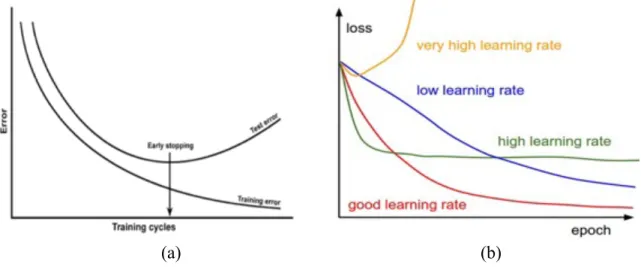
It is critical to design a hyperparameter profile for the BLSTM in order to avoid overfitting, also called overtraining. Overfitting occurs when a model learns the detail in the training data to the text that it negatively impacts the performance on testing data. On the contrary, underfitting, also called undertraining, refers to a model that can neither model the training data nor generalize to testing data (Brownlee, 2016). Figure 11a shows how overfitting would occur with respect to error over time (training cycles or epochs). The curve shows the testing error is significantly higher as the number of training epoch increases, indicating strong overfitting. When this happens, early stopping or limit the number of training epochs would avoid overfitting. Since the gradient of the weight matrix is updated at the end of each epoch, early stopping would produce a prediction output that fits the labels better. However, early stopping comes at the expense of increased error, because the loss function may not converge (Yao, Rosasco, &
Caponnetto, 2007). Applying regularization would be the more elegant approach: either a stronger L2 weight penalty, or more dropout, or collect more data (Karpathy, 2017).
(a) (b) Figure 11. Overfitting problem in training ANNs data (Karpathy, 2017).
Sometimes, high learning rate would result in overfitting problem as well (Figure 11b). A good learning rate leads to convergence of training loss.
Evaluation Metrics
Quantifying similarity between predicted heat maps and GT heat maps could be quite challenging. In this thesis, saliency evaluation measures were selected based on how frequent the measure appeared in the literature. Bylinskii et al. summarized most if not all similarity metrics and the three most referenced metrics are Area Under Curve (AUC), Linear Correlation Coefficient (CC), and Normalized Scanpath Saliency (NSS) (Zoya Bylinskii, 2017). Since the output of both prediction and GT are heat maps, AUC score was selected in order to compare how similar the maps are. Moreover, according to Hoberrock and Emami (2013), mean F-measure and L1 norm of the difference map are best suited for comparing predicted saliency map and reference salience map (Emami & Hoberock, 2013). Therefore, a total of three metrics was adopted in this thesis.
AUC score
AUC is the area under the Receiver Operating Characteristics (ROC) curve. Using this score, by thresholding over the GT and plotting true positive rate (TPR) vs. false positive rate(FPR), an ROC curve is achieved for each image. Then AUC score is averaged over all trained/tested images and the area underneath the final ROC curve is calculated. The math definition of AUC score is dependent on TPR and FPR and can be expressed as:
234 = 23 23 + 67; 634 = 63 63 + 27; 9:;< =)> = 1 7 234(634 @ ) A B A + ;
Perfect prediction corresponds to a score of 1 while a score of 0.5 indicates chance level.
Mean F-measure
The F-measure is the overall performance measurement and is computed as a weighted average of the precision and recall (sensitivity). Perfect prediction corresponds to a score of 1 while a score of 0 indicates a random pattern.
The precision, recall, and F-measure for evaluating saliency maps (S) from the network in comparison with GT (G) are given as follows (Figure 12):
Figure 12. Precision, Recall and F-measure equations
Where n is the number of correct pixel prediction (within allowed threshold) in S, NS is the number of total salient pixels in S, NG is the number of total salient pixels in G,
and C is the weighting that emphasized precision over recall. CD is chosen to be 0.3 in our
work to weigh precision more than recall (Achanta, 2009). L1 Norm of difference heat map
The difference heat map is generated by subtracting the pixel values of prediction heat map from the GT heat map, given the dimensions of both heat maps are the same (Emami & Hoberock, 2013). L1 norm of dissimilarity of a difference (error) heat map is defined as: EF + = G2(H, J) − 3KF(H, J) L M N O (P ∗ R) ;
hence the similarity of the difference(error) heat map is:
7EF = 1 − EF +
Summing up and taking the mean value is the metric of similarity of the heat maps, and this can be expressed as:
7EF = 7 − G2S(H, J) − 3KFS(H, J) L M N O (P ∗ R) A ST+
Another common evaluation metric is Normalized Scanpath Saliency (NSS). It’s the average of the response values at human eye positions in a model’s heat map (S) that has been normalized to have zero mean and unit standard deviation. Since proto-object saliency does not have higher-level information about object identity nor require eye fixation, NSS is not a relevant measurement for heat map evaluation.
EXPERIMENT I
Input representation and dimensionality
The input images, in binary representation, would be in a dimension of width (pixels) by length (pixels) by 3, with the three due to the red, green and blue color intensity. These input images vary from single object images to multi-object photos. To generate the input data for BRNN BLSTM training, each image is first converted into grayscale, then further processed into fixed-length vectors as input (Figure 14). These image conversion steps are the same as the post-processing of the POIS output heat maps described earlier.
Figure 14. A schematic diagram of generating input data
Model
Hyperparameters
BRNNs are advantageous in handling sequence data structure. In this study, the following hyperparameters are selected for training sequences of images windows:
Gradient Descent Hyperparameters: • Training iterations • Batch size • Loss function • Learning rate • Momentum Model Hyperparameters: • Number of Hidden units • Number of hidden layers
• Weight decay
• Activation function • Weight Initialization
• Dropout rate
Hyperparameter Assigned Values Expected Impact
Number of hidden Layers 2 for smaller dataset
4,6 for larger dataset How deep a network is to learn the general patterns. Number of layers depends on how complex the input-output relationship. Number of hidden units in
each hidden layer
128 or 256 for small dataset 256 or 512 for larger
dataset
Higher HLS will require more weights to be stored
Learning Rate 0.0001-0.001 Determines how quickly
or slowly the parameters are updated after each iteration
Number of outputs Varies depending on the
dataset, but should be in same dimension as the GT saliency maps
Prediction dimension should match those of the GT
Activation function Sigmoid, Relu or
combination of linear and non-linear
Logistic and ReLU are non-linear a.f. the proro-object features are most likely non-linear. The logistic activation would simulate the winner-takes-all implementation in JHU algorithm.
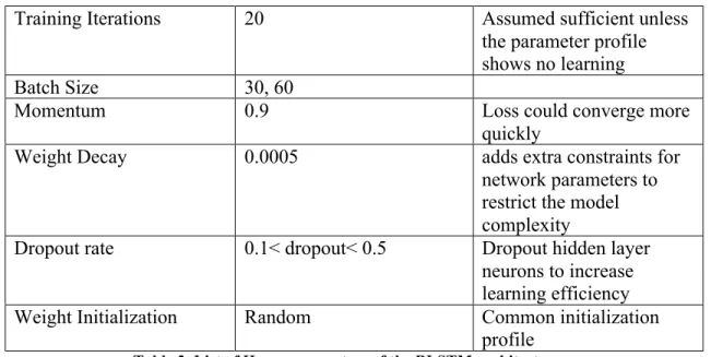
Training Iterations 20 Assumed sufficient unless the parameter profile shows no learning
Batch Size 30, 60
Momentum 0.9 Loss could converge more
quickly
Weight Decay 0.0005 adds extra constraints for
network parameters to restrict the model complexity
Dropout rate 0.1< dropout< 0.5 Dropout hidden layer
neurons to increase learning efficiency
Weight Initialization Random Common initialization
profile Table 2. List of Hyperparameters of the BLSTM architecture.
Number of hidden layers
Hidden layers are between the input layer and output layer. The number of hidden layers determines the depth of the network. For BRNNs, since there are both forward and backward hidden layers, the number of hidden layers is usually a multiple of 2. In this study, 2 to 4 hidden layers are explored initially, but was expanded to 4 to 6 later on. This is more than the number of hidden layers used in Cucciara’s SAM network (Cornia, Baraldi, Serra, & Cucchiara, 2016).
Number of hidden units in each hidden layer (HLS)
By default, mostly implementation of BLSTM uses 256 neurons/units for 2d data (images) or 1d data. The rule of thumb for selecting an optimal number of hidden units per hidden layer is (Heaton, 2008):
• The number of hidden neurons should be between the size of the input layer and the size of the output layer.
• The number of hidden neurons should be 2/3 the size of the input layer plus the size of the output layer.
• The number of hidden neurons should be less than twice the size of the input layer. Since the input layer contains sequences of length 1024 (or flattened 32 by 32 window), 256 or 512 are selected as HLS for LFSD dataset following the rule above. The value was kept the same when a CONV layer and a maxpooling layer were added.
Learning rate (LR)
Neural networks are often trained by gradient descent on the weights. This means, at each iteration, the derivative of the loss function with respect to each weight is
calculated by backpropagation and subtract it from that weight. Learning rate determines how quickly or slowly the parameters are updated after each iteration. A good learning rate is low enough such that the network converges to something useful, but high enough that you don't have to spend years training it.
Given the depth of the network and the HLS in each layer, a lower range of learning rate between 0.0001-0.001 is chosen in order to avoid overfitting (it learns everything just not useful), especially given that the training sample size in this study is not large.
Number of outputs
In the example of LFSD image dataset, each input image is an array of 360 by 360 by 3. They are preprocessed into a smaller window of 32 by 32 or a sequence of length 1024. The BLSTM will output the predicted saliency with sequences of length of 1024.
Activation function
Common activation function includes linear, rectified linear units (ReLU), logistic (sigmoid), tanh, etc. Saliency detection learning is assumed not to be linear and two non-linear activation functions, rectified non-linear unit (ReLU) and sigmoid are chosen to compare the performance. Also, a combination of sigmoid and linear activation function was considered.
Training iterations
For smaller training dataset, it is expected loss function (i.e. least square error) should converge within an iteration of 2-3 epochs and accuracy reaching close to 1 within 20 epochs. This is based on the BRNN network developed for handwritten digit
classifiers, indicating learning on image dataset can be done. Batch size (BS)
Since there are 60 images in the training set, a convenient value for batch size would be 30. This means the weight matrix values would be updated every 30 sequences. Momentum
The momentum parameter is useful in the case when training is stuck at a local minimum. It increases the size of the steps taken towards the minimum by trying to jump from a local minimum. If the momentum term is large then the learning rate should be kept smaller. A large value of momentum also means that the convergence will happen fast. Therefore, a momentum value of 0.9, which is a common choice to resolve the local minimum problem, would significantly reduce the number of epochs or quickly converge within the desired number of epochs (Orr, 2017).
Weight decay
Weight decay is essentially a parameter L2 norm (i.e. root mean square error) regularizer in computing L2. It adds extra constraints for network parameters to restrict the model complexity. Implementing weight decay would facilitate learning without increasing learning rate. A default decay of 0.0005 is selected.
Dropout rate (DR)
Dropout is a regularization technique where randomly selected neurons are dropped during training, and the activation of the downstream neurons is removed on the forward pass and thus the weight updates are not applied to these neurons on the
backward pass. Dropping crossed units would improve learning efficiently, making the network become less sensitive to specific weights of neurons to avoid overfitting. In this study, the dropout would be implemented on hidden layer rather than visible/input layer to allow all inputs be fed into the network without losing information. For image
classification, it is common to implement a dropout rate between 0.1-0.5 (would choose 0 by default). In this study, a dropout rate of 0 is chosen by default and would adjust to 0.1-0.5 in the case of overtraining the data.
Weight initialization
The wrong weight initialization will make gradients too large or too small, and make it difficult to update the weights and to the network’s convergence (Kumar, 2017). The most common choice for weight initialization is random (or Gaussian). If all weight were initialized to be the same (i.e. zeros or ones), every hidden units would receive the same signal and nothing useful would be learned (by definition, matrix multiplication
yields all zeros or ones). Random weight initialization breaks the symmetry and help the network to converge to the minimum. There are a few other weight initializations that are found to promote learning such as Xavier weight initialization (Glorot & Bengio, 2010) and layer-sequential unit-variance weight initialization (Mishkin & Matas, 2016)for CNN. Random weight initialization is selected for this thesis work.
Architecture
Figure 15 shows one of the four-layer BLSTM built for learning LFSD dataset
Figure 15. 4-hidden-layer BLSTM architecture
Design of Experiments
During the first phase of the saliency learning, the following hyperparameters were fixed: number of outputs (for LFSD images) is 1024, 20 training iteration, 0.9 momentum, adam as optimizer (adadelta would be a good alternative), L2 loss function with regularization of 1e -6, Weight decay = 0.0005. However, running a whole profile of
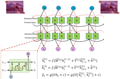
x0 x1 x2 xt A A A A yt A A A A y2 A A A A y1 A A A A y0 Forward State Forward State Backward State Backward State ℎ"($)= '(($ℎ "$)* + ,$ℎ")*$ + -$) ℎ"($)= '(($ℎ "$)* + ,$ℎ".*$ + -$) /0"= 1 2ℎ"+ 3 = 1(2[ ℎ"6; ℎ"(6)] + 3)
model parameters and gradient descent parameters would come out to be 72 experiments. To search for the optimal parameter settings, the following were taken into consideration:
1. With more hidden layers, lower learning rate would perform better.
This is the optimization surface becomes more complex as the number of hidden layers increase, therefore smaller learning rates are generally better. Although the loss would be stuck in local minima with low learning rate, it's much better than high learning rate for a more complex surface.
2. sigmoid and tanh are more prone to vanishing gradient problems, which can make learning much harder in deep neural networks (greater than 2 hidden layers).
3. Higher HLS would require higher learning rate, and therefore, would lead to overfitting. Lower HLS is better for generalizing
There are many rule-of-thumb (Heaton, 2008) methods for determining the correct number of neurons to use in the hidden layers, such as the following:
1. The number of hidden neurons should be between the size of the input layer and the size of the output layer.
2. The number of hidden neurons should be 2/3 the size of the input layer, plus the size of the output layer.
3. The number of hidden neurons should be less than twice the size of the input layer.
Based on the above the number of experiments were cut down to 24 runs, and they are summarized in Table 3.
BLSTM hyperparemeter profile model GD Lr = 1e-4 Bs = 30 Lr = 1e-4 Bs = 60 Lr = 5e -4 Bs = 30 Lr = 5e-4 Bs = 60 Lr = 1e -3 Bs = 30 Lr = 1e -3 Bs = 60 model GD # hidden = 4 hls =128 Loss fun =relu
# hidden = 2 hls =128 Loss fun =relu # hidden = 4
hls =256 Loss fun =relu
# hidden = 2 hls =256 Loss fun =relu # hidden = 4 hls =128 Loss fun =sigmoid+linear # hidden = 2 hls =128 Loss fun =sigmoid+linear # hidden = 4 hls =256 Loss fun = sigmoid+linear # hidden = 2 hls =256 Loss fun = sigmoid+linear Table 3. BLSTM parameter profile for LFSD dataset
Training Results
Initially, AUC scores for many of the trained BLSTMs were close to 0.5, indicating the result was no more than random guessing. Table 4 showed learning saliency from sequences of pixel values was not successful.
BLSTM hyperparemeter profile model GD Lr = 1e-4 Bs = 30 Lr =1e-4 Bs = 60 Lr = 5e-4 Bs = 30 Lr = 5e-4 Bs = 60 Lr = 1e-3 Bs = 30 Lr = 1e-3 Bs = 60 model GD # hidden = 4 hls =128 Act fun =sigmoid 0.512 0.533 0.512 0.533 0.500 0.500 # hidden = 2 hls =128 Act fun =sigmoid # hidden = 4 hls =256 Act fun =sigmoid 0.527 0.539 0.527 0.539 0.502 0.503 # hidden = 2 hls =256 Act fun =sigmoid #hidden = 4 hls =256 Act fun =relu
0.509 0.511 0.500 0.501 0.485 0.402 #hidden = 2
hls =256 Act fun =relu Table 4. AUC score for LFSD dataset training (without normalization & CONV layer)
EXPERIMENT II
GT heat maps
Because of the change in input size to the BLSTM network, the GT heat maps were resized into the same shape as the prediction feature matrix (89x89), which was concatenated and converted to grayscale (integer with values from 0-255) as well for post-processing.
Meanwhile, during the experimentation it was observed that the level of saliency needed in the GT label set would affect training. Simply, BLSTM gave different output when training with higher pyramid level compared to lower ones. As previously
mentioned in the section of GT saliency images, the value of M or pyramid level would reduce the number of pixels (smaller image matrix and therefore smaller sequences) to train. In phase II of the experiment, we kept the same parameters for generating GT heat maps.
Model
Architecture
BLSTM would learn more effectively on input composed of convolutional filters than input with pixel vectors. The advantage of using convolutional layer/filter lies in its ability to facilitate network to learn to recognize images. Since the development of LeNet, one of the very first CNN that helped propel DL, multiple convolutional layers along with maxpooling layers allow programs to recognize digits, objects, boundaries, edges, etc. This shift of what input to use changed the training performance of BLSTM.
Since the first round of training did not produce the desired learning, a CONV layer is added on top of BLSTM instead of feeding the fixed-length vectors from the grayscale image to BLSTM. As CNNs are designed to learn feature from the spatial domain in images, they could generate feature maps (from heat maps) that would
improve BLSTM learning. For each LFSD image, which has a dimension of 360x360x3, was convolved with a flattened fixed-length filter (or kernel) of 147 (7x7x3) at a stride of 2. Normal filter sizes (3 by3 in VGG, 7 by 7 in ZFnet, and 11 by 11 by Alexnet) are efficient for CNNs to extract features, so a similar filter size was considered for this phase of the experiment (Simonyan & Zisserman, 2014) (Zeiler & Fergus, 2013) (Krizhevsky, Sutskever, & Hinton, 2012). The number of kernels was selected to be 64 for two reasons: one followed the filters designed to extract features from handwritten digit classification (MNIST) and the other was to mimic the odd and even BO kernels (multiple of 8) in POIS. Then stretching this filter along both width and height led to a 178 by 178 feature map. The weight matrix for CONV layer was of size 64 by 147 (length of the flattened filter), and by filter-wise multiplication with ReLU activation (Zeiler & Fergus, 2013) yielded a 64 by 31684 (or 178x178) activation map.
A maxpooling layer, or a down-sampling layer was added right after the CONV layer. The pooling layer filter was selected to be 2 by 2 with a stride of 2 following the logic by the ZFnet (Zeiler & Fergus, 2013), and this reduced the total parameters in the network by 75%. The output of this maxpooling layer was 64 by 7921 (the square of (178