Methods for statistical and population genetics
analyses
by
Shyam S. Gopalakrishnan
A dissertation submitted in partial fulfillment of the requirements for the degree of
Doctor of Philosophy (Biostatistics)
in The University of Michigan 2011
Doctoral Committee:
Associate Professor Sebastian K. Zoellner, Chair Professor Michael L. Boehnke
Associate Professor Zhaohui Qin
c
Shyam S. Gopalakrishnan 2011 All Rights Reserved
ACKNOWLEDGEMENTS
I want to express my gratitude to all the people who made this dissertation possible. I would like to thank my advisors, Drs. Steve Qin and Sebastian Z¨ollner for their support and advice throughout the course of my graduate studies. Steve made my transition from Engineering to Biostatistics a smooth one, teaching me the nuances of the field along the way. I have Sebastian’s class to thank for my strong interest in population genetics. His mentorship during my dissertation work has been instru-mental in the formation of my academic temperament. I would also like to thank my dissertation committee for providing me with feedback and suggestions. In particu-lar, I would like to thank Dr. Michael Boehnke, for taking the time to advice me on various subjects.
Just as “it takes a village to raise a child”, it takes an entire department to com-plete a dissertation. I have made several good friends during my stay in Ann Arbor. Matthew Zawistowski and Tanya Teslovich have been trusted friends without whom this journey would not have been half as interesting. I can only hope to find colleagues such as Rui, Jun, Weihua, Abby, Mark, Rob, Matthew, Anne, Wei and Heather. This thesis would not have come to fruition without the help of Sue Burke and Dawn Keene, who were there to help me with matter small and big.
I would like to thank my family for their steadfast support even when it looked like I would never finish. I draw my strength from my mother and father, the best
teachers that I could have asked for. My sister, Shubha, has been a confidante my entire life. Finally, I would like to thank my rock, Roshni, for all her support during all the ups and downs of my life.
TABLE OF CONTENTS
DEDICATION . . . ii
ACKNOWLEDGEMENTS . . . iii
LIST OF FIGURES . . . vii
LIST OF TABLES . . . ix
CHAPTER I. Introduction . . . 1
1.1 Scope of this dissertation . . . 2
II. An efficient comprehensive search algorithm for tagSNP se-lection using linkage disequilibrium criteria . . . 5
2.1 Introduction . . . 5
2.2 Methods . . . 7
2.3 Results . . . 14
2.4 Discussion . . . 18
III. Framework for remapping multiply mapped short reads . . . 22
3.1 Introduction . . . 22
3.2 Methods . . . 24
3.3 Results . . . 29
3.4 Discussion . . . 31
IV. Feasibility of admixture mapping to identify rare susceptibil-ity variants . . . 34
4.1 Introduction . . . 34
4.3 Results . . . 52
4.4 Discussion . . . 54
V. Estimating site frequency spectra from low coverage sequenc-ing data . . . 62 5.1 Introduction . . . 62 5.2 Methods . . . 65 5.3 Results . . . 72 5.4 Discussion . . . 74 VI. Conclusion . . . 80 BIBLIOGRAPHY . . . 84
LIST OF FIGURES
Figure
2.1 Example configuration where greedy approach does not pick the least number of tagSNPs . . . 9
3.1 Proportion of multiply mapped reads aligned to their true location using our algorithm . . . 31
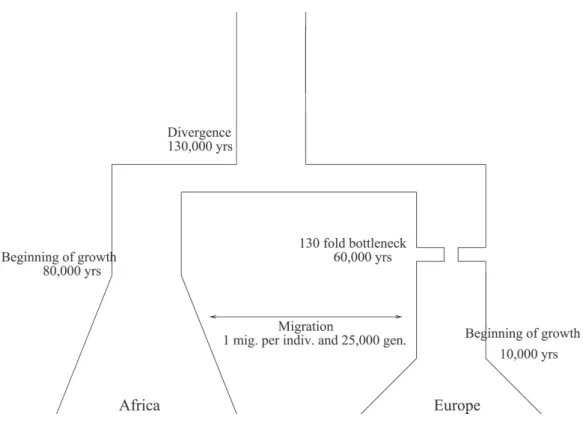
4.1 Admixed chromosomes and admixture blocks . . . 36 4.2 Population model used for simulating haplotypes usingms . . . 49 4.3 Relative risk vs minor allele frequency. Power of single marker test is
set at 10% for 20000 cases and controls, correcting for 1 million tests. 51 4.4 Contour plot showing the power of admixture mapping against the
contribution to prevalences in the two founding populations. The power of admixture mapping is shown for two different mixing ratios of 80%-20% and 50%-50%. . . 57
4.5 The relationship between power of admixture mapping and contribu-tion to prevalence in populacontribu-tion A, plotted for various sample sizes. The contribution to prevalence in the second population was fixed at 1%. . . 58 4.6 Mean ratio of contribution to prevalences in the African population
vs the European population plotted against the cumulative risk allele frequency. The contribution to prevalence in Europeans was fixed to 1%. . . 59
4.7 Power of admixture mapping compared to the power of single marker tests (blue lines) in Europeans. Two levels of European ancestry were considered, 20% (red lines) and 50% (black lines). The hollow symbols represent tests with 1000 cases and 1000 controls, whereas the filled symbols represent test with 10000 cases and controls each. 60
4.8 Power of admixture mapping compared to indirect association. Sam-ple size was 5000 cases and controls each. TagSNPs were chosen with two minor allele frequency cutoffs, 1% and 0.5%. . . 61 5.1 Estimated SFS using individual based genotype calls using 200
sam-ples sequenced at 30-fold average depth . . . 73 5.2 Estimated SFS for low pass, 4-fold, short read sequencing data. The
panels show the first 10 bins of the estimated SFS using genotypes from (a) an individual level caller, (b) population level caller and (c) population level LD aware caller. . . 76
5.3 MLE estimate of the SFS using simulated data . . . 77 5.4 Mean and standard error of the ratio of true to estimated SFS for
each bin . . . 78 5.5 QPOC data: Comparison of MLE and counting estimate of SFS . . 79
LIST OF TABLES
Table
2.1 Summary of Chromosome 2: Number of tagSNPs with greedy ap-proach and FESTA . . . 18
2.2 TagSNP distribution on Chromosome 2: Number of tagSNPs per precinct. . . 19
2.3 Summary of tagSNP results for Encode regions: CEU samples . . . 19 2.4 Comparing different criteria for tagSNP selection: Effect on number
of tagSNPs in denser SNP maps . . . 20 3.1 Population parameters for simulating short read sequence data . . . 29 3.2 Read characteristics for chromosome 21 simulated data . . . 30
3.3 Effect of multiply mapped reads on variant discovery . . . 32 5.1 Expected SFS bin counts under neutral and our parameterization . 67
CHAPTER I
Introduction
One of the major goals in the field of genetics is to identify disease predisposing genetic variants, to better understand the underlying mechanism and ultimately identify tar-gets for intervention. Aided by advances in technology, the tools used to accomplish these goals have rapidly evolved.
Risch and Merikangas [1] first advocated the use of large scale association studies to detect disease predisposing variants. Large scale association studies were not feasi-ble at the time. Since then, the advances in high throughput low cost genotyping have propelled association studies, especially genome-wide association studies (GWAS), to become the instrument of choice in disease genetics.
GWAS have been highly successful in identifying variants associated with a wide array of common diseases and quantitative traits, e.g. type 2 diabetes[2], Parkinson’s disease, LDL cholesterol etc[3]. GWAS are best suited to identify variants that fall under the Common Disease Common Variant (CDCV) hypothesis. The CDCV hy-pothesis states that the prevalence of common diseases can be attributed to a few common variants with moderate effect sizes. Though GWAS have identified more than 4900 associated loci for more than 200 traits, these common variants explain
only a small fraction of the heritability of the common diseases[4, 5].
The presence of rare causal variants has been suggested as a possible source for the missing heritability. GWAS are not well powered to detect rare variants. The Common Disease Rare Variant (CDRV) hypothesis suggests that common diseases can be explained by multiple rare variants with large effect sizes[6]. Several methods have been proposed to identify rare causal variants[7, 8]. Since testing individual rare variants is not statistically powerful, most methods collapse information across multiple rare variants. Development of new methods to identify rare susceptibility variants remains an area of much interest.
The search for rare susceptibility variants was further expedited by the emergence of short read sequencing[9]. Short read sequencing technologies allowed low cost large scale sequencing. Sequencing studies have been used to catalog variants in the human genome [10], identify rare causal variants for traits such as LDL and HDL cholesterol[11, 12], quantify gene expression [13], identify DNA protein interaction[14] and perform population genetics studies [15]. Analysis of short read sequence data present many interesting statistical challenges.
1.1
Scope of this dissertation
In this dissertation, I present novel methods aimed at tackling some of the statistical challenges in the field of genetics.
TagSNP Selection
Association studies rely on indirect association to maintain power. They test a rep-resentative set of markers, tagSNPs, in lieu of all the variants in the genome. The
power of association tests using tagSNPs is directly proportional to the linkage dis-equilibrium measure r2 between the tagSNP and the causal variant. In chapter 2,
we propose a graph-based method to select the optimal set of tagSNPs. We define optimality in terms of the number of tagSNP markers. We use a ”divide and con-quer” approach to identify the smallest set of tagSNPs that is highly correlated with all the variants in the region. As an example, we apply our method to chromosome 2 HapMap [16] data and ENCODE regions.
Remapping multiply mapped reads
The alignment of short reads is dependent on many factors like read length and error model. Further, the presence of repetitive elements and structural variants on the reference sequence results in a fraction of short reads being aligned to multiple loca-tions in reference. These multiply mapped reads are often discarded.
In chapter 3, we present a Gibbs sampling approach to identify the most likely ge-nomic location for multiply mapped reads. Additional information from the multiply mapped reads can improve the performance of downstream analyses. We illustrate the effect of including multiply mapped reads using variant discovery in a simulated sample.
Admixture mapping to identify rare variants
An admixed population derives its ancestry from multiple founding populations. Ad-mixture mapping is a tool that identifies regions associated with the disease by testing the correlation of the ancestry of the region with the disease status.
Methods designed to detect rare causal variants combine information across multiple markers. Several strategies exist to collapse across markers, viz., presence of minor
allele, sum of minor alleles, sum of weighted allele frequencies etc. Ancestry across a testing unit can be construed as a way to summarize the information contained in the markers in the region. In chapter 4, we explore the power of admixture mapping to detect regions harboring multiple rare causal variants. We propose a disease model for the rare causal variants. In settings unsuitable for single marker association tests, we test the feasibility of admixture mapping to detect the rare susceptibility loci.
Site frequency spectrum estimation
The site frequency spectrum (SFS) is a population genetics statistic that contains information on the number of variant positions at each minor allele frequency in the sample. The SFS is an important summary statistic in population genetics, encom-passing information on selection and demographic history. All population genetics statistics that do not include linkage disequilibrium information can be expressed as functions of the (SFS). Estimates of the SFS obtained from genotyping platforms suf-fer from ascertainment bias, since there exist potentially variable positions that are not included on the genotyping array. Since all positions are queried in a sequencing study, SFS estimated from sequencing studies do not suffer from ascertainment bias.
In chapter 5, we present a maximum likelihood estimation procedure to the estimate the SFS from low coverage short read sequence data. First, we show that estimates of the SFS obtained from genotype calling methods underestimate the number of rare variants, especially singletons and doubletons. We demonstrate that our method performs better than SFS obtained from genotype calling algorithms using both sim-ulated and real data examples.
CHAPTER II
An efficient comprehensive search algorithm for
tagSNP selection using linkage disequilibrium
criteria
2.1
Introduction
Genome-wide association studies have emerged as the predominant approach to detect genetic variants that contribute to human diseases. Initially, genome-wide associa-tion studies focused on single nucleotide polymorphisms (SNPs) because of their high abundance in the human genome, their low mutation rates and their accessibility to high-throughput genotyping [17]. There are more than 10 million verified SNPs in dbSNP (build 124)[18], but typing all available SNP markers is inefficient and unnec-essary since many will provide redundant information due to linkage disequilibrium (LD). A better strategy is to select a subset of representative SNPs (tagging SNPs or tagSNPs) and to remove the rest from consideration [19, 20]. The objective is to have little information overlap among the selected SNPs while retaining much of the signal contained in the original set.
and Carlson et al. [36] introduced methods based on the LD measure r2. These
methods search for a small set of SNPs that are in strong LD (measured through pairwise r2) with other SNPs that are not selected for genotyping. Pairwise r2 is an
attractive criterion for tagSNP selection since it is closely related to statistical power for case-control association studies, where a directly associated SNP is replaced with an indirectly associated tagSNP [6].
In this manuscript, we describe efficient algorithms for tagSNP selection based on pairwise LD measure r2. The algorithms were implemented in a computer program
named FESTA (fragmented exhaustive search for tagging SNPs). Essentially, we re-place a greedy search, where markers are added sequentially to the tagSNP set, with an exhaustive search where all marker combinations are evaluated. To achieve this, we arrange the genome into precincts of markers in high LD, such that markers in dif-ferent precincts show only low pairwise disequilibrium. TagSNP selection can then be performed within each precinct independently, greatly reducing computation cost. In most settings, our method is guaranteed to find the optimal tagSNP set(s) defined by the r2 criterion. For a small proportion of precincts where exhaustive search is
com-putationally too expensive to carry out, an efficient greedy-exhaustive hybrid search algorithm is described. Using data from the HapMap project [16], we show that the majority of these precincts contain relatively small numbers of SNPs, especially when a stringent r2 criterion is used. Our algorithm readily identifies equivalent tagSNP
sets, so that additional selection criteria can be incorporated. Other useful extensions are also discussed in this manuscript, such as the inclusion/exclusion of certain SNPs and double coverage, which can increase robustness of tagSNP sets against sporadic genotyping failures or errors.
2.2
Methods
Consider a set S which contains M bi-allelic SNP markers a1, a2, . . . , aM. Further
assume that all these markers have minor allele frequency (MAF) above a certain threshold (0.05 was used in this study). First, two-SNP haplotype frequencies were estimated [37], and then the pairwise LD measure r2 (also referred to as D2) [38]
was calculated for each pair of markers using the inferred haplotype frequencies [39]. Two markers ai and aj are said to be in strong LD if the r2 between them is greater
than a pre-specified threshold value r0, denoted as r2(ai, aj)≥r0 (r0 = 0.5 or 0.8 in
in this study). Both are considered tagSNPs for each other; i.e. ai can be used as a
surrogate for aj, and vice versa.
Our aim is to a find tagSNP set, denoted by T, a subset of S such that ∀ai ∈ S\T, ∃aj ∈ T that satisfies r2(ai, aj) ≥ r0. In our presentation, we introduce two
intermediate SNP sets, P andQ. P is called the candidate set which contains all the markers that are eligible to be chosen as tagSNPs andQis named the target set which contains all the markers that are yet to be tagged, i.e. no marker in Q is in LD with any tagSNP inT. For each markeram inP, letC(am) :={a:a∈Q&r2(a, am)≥r0}
represent the subset of Q which contains markers that are in strong LD witham, and
let |C(am)|be the number of the elements in the setC(am). Typically, the candidate
set P is the complement of the tagSNP set T, P = S\T and P = Q. One
excep-tion occurs when some SNPs are excluded as tagSNPs because they cannot be easily genotyped, but they still should be tagged by other markers if possible. In this case, the candidate set is a subset of target set. We describe several different algorithms for updating P, Q and T starting with a greedy approach [36]. We then outline successive refinements and extensions of a partition and exhaustive search algorithm, designed to handle various scenarios encountered when planning association studies.
2.2.1 Greedy Approach
The detailed algorithm is as follows [36].
Algorithm 1 (greedy approach):
1. Set T =∅ and P =Q=S.
2. For each marker am ∈P, calculate |C(am)|.
3. For every marker am where|C(am)|= 0, addam intoT, and remove it fromQ.
4. Find the marker in P that has the highest |C(am)| value, denoted asamax, and
add amax into T, removing it and all connected SNPs, i.e. C(am) from Q. (5)
Repeat Steps 2-4 until Q=∅.
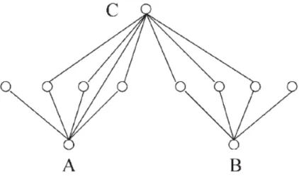
In Step 4, by removing associated markers from consideration, the coverage overlap among tagSNPs is greatly reduced. Although it is simple to implement, the greedy procedure may miss more efficient solutions. Figure 2.1 gives a simple example, where markers A and B each tag half of all markers and together can tag all the markers. However, marker C is connected to more than half of all markers, and it is the first marker selected by the greedy algorithm. In this example, the greedy algorithm produced a set with three tagSNPs, despite the fact that the optimal solution contains only A and B.
2.2.2 Exhaustive search
An exhaustive search guarantees the minimum tagSNP set. Therefore, theoretically, the exhaustive search solves the tagSNP selection problem. But in practice, genome-wide tagSNP selection requires consideration of hundreds of thousands of SNP mark-ers. For problem of this scale, exhaustive searches cannot be directly applied due to
Figure 2.1: Example configuration where greedy approach does not pick the least number of tagSNPs
prohibitive computation costs.
Since appreciable LD only occurs within clusters of nearby markers along chromo-somes, a practical solution is to first decompose the set of markers into disjoint precincts, such that markers in different precincts are never in strong LD. Then, selecting tagSNPs using the r2 criterion in the whole set is equivalent to selecting
tagSNPs in each precinct and then combining all the tagSNPs together. Here the concept of precinct is defined based on pairwise LD measure. It is therefore closely related to haplotype blocks [40, 21, 41, 42, 23, 43], which are regions where historical recombination events are rare. The main difference is that the precincts of markers in high r2 are determined purely based on satistical correlation. Unlike haplotype
block, markers within each precinct may not be consecutive markers sitting next to each other.
in graph theory. We applied the Breadth First Search (BFS) algorithm [44]. Starting from any node (a marker) in a new precinct, this algorithm adds all neighboring nodes (markers in LD) and all neighbors of the newly added nodes to the precinct, until there are no neighbors to be added to the precinct. This process is restarted from different nodes until all the nodes are assigned to a precinct.
After the partitioning step, we perform the tagSNP selection within each precinct. Starting with K = 1, allK-marker combinations are searched to see if they cover all markers within this precinct. If not, K is increased by one and the search is repeated until a tagSNP set is found or a pre-specified search limit is reached.
When evaluating all K-marker combinations, the computation cost required for an exhaustive search might be too great in some precincts. In such cases, we propose a hybrid solution which reduces the computation cost and retains a good chance of finding optimal tagSNP sets. For each precinct i with Ni markers (Here on, all
pa-rameters with subscript i indicate parameters within the i-th precincts, such as Ki,
Ji,Pi, Qi,Ti and Ni.), we decide whether an exhaustive search is feasible by
compar-ing the computation cost required for evaluatcompar-ing all K-marker combinations within a precinct, Ni
K
, with a computation cost limit Lspecified a priori, determined based on available computing resources. Larger limits allow a more comprehensive search, which may result in fewer tagSNPs being selected, but require additional computa-tional effort. In this study, we set this limit at 1 million. When this limit is exceeded, we apply the following hybrid algorithm. SpecifyK∗
i such that it is the largestK
pos-sible that satisfies Ni
K
≤L0 , whereL0 is a pre-specified computation cost limit (less
than L, set at 10000 in studies conducted here). Subsequently, for each K∗
i-marker
combinations, denoted as {a1. . . aK∗
i}, assume that these markers have already been
target set Qi, m = 1. . . Ki∗, i.e. Pi = Qi = Si SK ∗
i
m=1(am ∪C(am)), then apply the
greedy approach to identify a subset of Pi that is able to cover Qi, which contains
the remaining untagged markers.
The tagSNP set obtained in the reduced set plus the previous K∗
i markers together
form a complete tagSNP set for thei-th precinct. The detailed algorithm is as follows:
Algorithm 2 (FESTA: greedy-exhaustive hybrid search):
1. Apply the Breadth First Search to decompose the entire set of markers into precincts such that high LD can only be observed within precincts. S =
S
nSi, andSi∩Sj =∅f oralli6=j
2. Within each precinct Si, set K = 1,
a If Ni
K
≥ L, move to (b), otherwise conduct an exhaustive search over all possibleK-marker combinations. Both the candidate setPi and the target
setQi are Si. If no combination of K SNPs can cover the entire precinct,
setK =K+ 1, and repeat this step. b Find K∗ i such that KNi∗ i ≤ L0 and KN∗i i+1
> L0. For every Ki∗ marker
combination in Si, denoted as {a1. . . aK∗
i}, let Ti = ∪m{am}, Pi = Qi =
Si\SKi∗
m=1({am}∪C(am), and apply the greedy approach to identify a subset
ofPi that is able to cover the remaining untagged markers Qi. Among all
the resulting tagSNP sets, we choose the smallest set.
3. Record all minimum tagSNP sets that cover the precinct. These form the complete minimum tagSNP sets{Tij :j = 1. . . Ji}, whereJi is the total number
of such minimum tagSNP sets.
tagSNP set for the whole setS. Suppose the size of the minimum tagSNP set(s)
in each precinct is Ki, then the overall size of such minimum tagSNP sets is
Pn
i=1Ki, and the total number of such minimum tagSNP sets is Qni=1Ji.
FESTA executes either a pure exhaustive search or a greedy-exhaustive hybrid search in each precinct depending on the computational cost. Exhaustive search is first at-tempted, and if the computation cost becomes too high, the hybrid algorithm is used as a fall back. Typically, only a small proportion of the precincts require the greedy-exhaustive hybrid search.
2.2.3 Additional features
Mandatory tagSNP markers
Our algorithm readily allows users to force certain mandatory SNP markers to be included or excluded in the tagSNP set. There are several scenarios where such func-tionality is important. First, in candidate gene studies, previous knowledge may be available as to which SNPs are functionally important. These might include non-synonymous coding region SNPs (cSNPs) as well as SNPs located in regulatory re-gions. Second, in genome wide studies, one might carry out multiple rounds of geno-typing and tagSNP selection. In such cases, additional tagSNPs could be selected at each round to cover the markers not tagged by tagSNPs successfully genotyped in the previous round. We provide an example of this in the results section. In other settings, it may be useful to exclude certain SNPs from consideration as tags. For example, some SNP markers may be difficult to genotype using a particular platform.
When there are mandatory markers{t1, . . . , tr}to be included, add these markers into
the tagSNP set T, and remove them from the candidate set, i.e. P = P\Sr
i=1{ti}.
The target set Q =Q\Sr
to be excluded from the tagSNP set, we simply remove them from the candidate set, the target set Q is unchanged.
Choosing between alternative solutions
Within a densely typed SNP set, redundant tagSNPs are common, which results in multiple tagSNP sets of the same size. All of these sets are equal in the sense of min-imizing the number of tagSNPs. In order to choose one set for genotyping, additional criteria can be employed. Here we evaluate several alternative criteria:
1. Maximize average r2 between tagSNPs and untagged SNPs they represent
2. Maximize the lowest r2 between tagSNPs and the untagged SNPs they cover
3. Minimize the average r2 among all pairs of tagSNPs within a precinct
4. Maximize the average r2 among all pairs of tagSNPs within a precinct
5. Maximize the average minor allele frequencies among all tagSNPs
In criteria 1 and 2, we try to identify the tagSNP sets that have the strongest connec-tions with those untagged SNPs, which should increase power on average and in the worst case respectively. The purpose of using criteria 3 is to find a tagSNP set whose members are as independent as possible which minimizes overlap between tagSNPs and potentially increases the chance of linking to untyped SNPs. Criteria 4 may increase redundancy and robustness to genotype failure; and criteria 5 may improve genotyping success for some assays.
To evaluate the relationship between each tagSNP set identified by the aforementioned criteria, and more importantly, their potential of uncovering the disease causing mu-tations in association studies, we conducted some empirical evaluations, summarized in the Result section.
Other types of criteria may be of even greater interest in practice. For example, in many genotyping technologies, some SNPs are harder to genotype than others due to characteristics of surrounding genome sequence. We can use this information to select tagSNPs that are likely to have a high success rate, and to avoid SNPs that are prone to genotyping failure.
Double Coverage
So far, both the greedy approach and our FESTA algorithm focus on finding a tagSNP set such that each SNP is either a tagSNP itself or is in LD with at least one of the tagSNPs. This is a criterion aimed at minimizing the number of tagSNPs selected. In reality, random genotyping failure or genotyping error on these tagSNPs can result in loss of power to identify the true signal. To be more robust against such adverse events, we evaluated a more stringent criterion requiring that every untyped SNP be in LD with at least two tagSNPs.
Our FESTA algorithm can be extended to find tagSNP sets that will have double coverage on the SNP markers considered. As always, an exhaustive search is able to find such tagSNP sets when the marker set considered is not too large. When ex-haustive search is not feasible, the same greedy-exex-haustive hybrid search strategy can be applied. In practice, it may be useful to consider double coverage only for large precincts, where the cost of losing an SNP to genotyping failure might be higher.
2.3
Results
To illustrate our proposed piecewise exhaustive search strategy, compare it with the greedy approach and explore the various characteristics of the tagSNP sets selected by our method, we applied both methods to two sets of data, the entire Chromosome
2 and five ENCODE regions (ENr112, ENr131, ENr113, ENm010 and ENm013) geno-typed by the HapMap project (release 16c, June 2005). All three populations: CEU (European), YRI (Yoruban) and JPT + CHB (Japanese and Chinese) were studied. The first is in the context of a genome-wide association study and the second is sim-ilar to the situation of a candidate region study.
2.3.1 Chromosome wide tagging
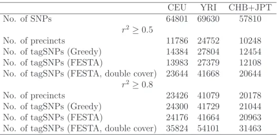
We have applied the greedy algorithm and FESTA to Chromosome 2 using HapMap Phase 1 genotype data (release 16c, June 2005). Tables 2.1 and 2.2 summarizes the results. FESTA produces fewer tagSNPs compared with the greedy approach in all three populations. When compared across populations, the YRI samples have about twice the amount of tagSNPs as the CEU or the JPT+CHB samples. The JPT+CHB samples have slightly less tagSNPs identified than the CEU samples. With r2
thresh-old 0.5, the percentages of tagSNPs identified by our algorithm are 21.6% in CEU, 39.3% in YRI and 20.9% in JPT+CHB samples, respectively.
The size of the tagSNP set is optimal for precincts where the greedy approach indi-cates that one or two tagSNPs are enough to cover all the SNPs in it. Improvements over the greedy approach is only possible for the remaining precincts. In the CEU samples, there are 599 of such precincts, in which the greedy approach identified 2423 tagSNPs, and FESTA identified 2022, a 16.5% reduction. When the r2
thresh-old is 0.8, 154 precincts require more than two tagSNPs, as identified by the greedy approach. Among them, the greedy approach and FESTA identified 526 and 402 tagSNPs, respectively, a reduction of 23.6% in tagSNPs chosen by FESTA. When double coverage is required, 69.1% and 45.9% more tagSNPs are needed with r2
and JPT + CHB samples.
Among all the non-singleton precincts in the CEU samples (6545 for r2 threshold of
0.5 and 10196 forr2 threshold of 0.8), most require only a small number of tagSNPs,
so that the exhaustive search can be applied directly. With r2 threshold of 0.5, the
greedy-exhaustive hybrid approach was required for only 98 precincts or 1.5% of all precincts (11 precincts (0.1%) with r2 threshold of 0.8).
2.3.2 Densely typed region
A dense SNP map was released by the HapMap project on the ENCODE regions. We used five such regions (ENr112, ENr131, ENr113, ENm010 and ENm013) to evaluate the performance of our algorithm. Each ENCODE regions is 500 kb in length, for the CEU samples, the average number of SNPs in these regions is 832 (ranges from 551 to 1126), corresponding to an SNP density about 1 SNP per 601 bps (1 SNP per 907 bps to 1 SNP per 444 bps for individual regions). The detailed results were summarized in Table 2.3. In this set of densely typed SNPs, using our method with
r2 threshold of 0.5, the average percentage of tagSNPs required to cover each of the
five regions is 8.3% of all markers (ranges from 5.4 to 11.3%). For double coverage, on average, 76.7% more tagSNPs are required (ranges from 70.7 to 83.6%). With a more stringent r2 threshold of 0.8, the average percentage of tagSNPs required increased
to 16.6% of all markers (ranges from 11.4 to 24.1%). To double cover these regions, 62.9% more tagSNPs are required (ranges from 56.9 to 71.6%). For precincts where improvement over greedy search is possible, using FESTA, the improvement in the number of tagSNPs is 17.9 and 23.0% on average for the five ENCODE regions with
r2 thresholds of 0.5 and 0.8 respectively. Using our method on YRI and JPT + CHB
2.3.3 Additional TagSNPs for denser SNP map
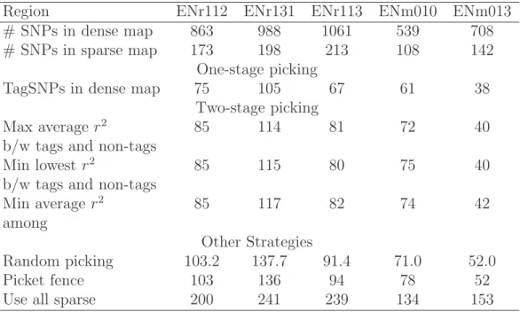
With the improvement in genotyping technologies and discovery of rarer variants, progressively denser SNP maps will become available. As more refined association studies are carried out, it will be useful to select new tagSNPs to ‘fill holes’ in the initial sparse maps. With a good picking strategy for the first round of tagging, this staged approach should result in only a small-to-moderate increase in the total num-ber of tagSNPs compared to a one-stage strategy.
To evaluate this strategy, we constructed an artificial sparse SNP map for each of the five ENCODE regions (using the CEU samples only). Specifically, we selected one in every five consecutive SNP markers. The density of this sparse map is about 1 SNP per 3kb, close to the density of the phase I HapMap. Then, three different tagSNP sets are identified using the three criteria described previously, denoted by
Ti, i= 1, 2, 3. Finally, we applied our approach to the full ENCODE SNP set, using
each of these tagSNP sets as a seed, to search for additional tagSNPs to cover the previously ‘hidden’ SNP markers. The effectiveness of these tagSNP sets is evalu-ated by comparing the number of new tagSNPs needed to cover the ‘newly found’ SNPs. In addition to the three criteria, we also compared three other tagSNP selec-tion strategies: Z random SNPs, assume Z is the number of tagSNPs for the sparse map, a picket fence strategy with Z equally spaced SNPs, where we place equally spaced grid points along the interval and then select markers that are closest to these grid points or using all original SNPs as tagSNPs. The results are summarized in tables 2.4. When the r2 threshold is 0.5, 14.4% more tagSNPs (range from 7.0 to
20.9%) are needed to fill holes in the original map and that number is only 5.4% (range from 3.8 to 7.0%) with an r2 threshold of 0.8. The three tagSNP sets require
CEU YRI CHB+JPT
No. of SNPs 64801 69630 57810
r2 ≥0.5
No. of precincts 11786 24752 10248
No. of tagSNPs (Greedy) 14384 27804 12454 No. of tagSNPs (FESTA) 13983 27379 12108 No. of tagSNPs (FESTA, double cover) 23644 41668 20644
r2 ≥0.8
No. of precincts 23426 41079 20178
No. of tagSNPs (Greedy) 24300 41729 21044 No. of tagSNPs (FESTA) 24176 41664 20963 No. of tagSNPs (FESTA, double cover) 35824 54101 31463
Table 2.1: Summary of Chromosome 2: Number of tagSNPs with greedy approach and FESTA
fewer tagSNPs to cover the holes, compared with tagSNPs picked using a picket fence strategy (31.6% difference for r2 threshold of 0.5 and 21.6% difference for r2
thresh-old of 0.8) or picked at random (33.8% difference for r2 threshold of 0.5 and 21.0%
difference for r2 threshold of 0.8).
2.4
Discussion
In this manuscript, we developed an efficient computational framework for tagSNP selection using the r2 criteria. Our algorithm can handle 100,000s of linked markers
and can identify smaller tagSNP sets than the greedy approach [36]. Using both chro-mosome wide data and densely typed ENCODE data from HapMap, we illustrated the utility of our approach and showed savings increase in more densely typed regions and inside large LD “blocks”. Computational effort required by our method can be tailored to available computing resources. Another important feature is the ability of our method to identify multiple equivalent tagSNP sets and use additional criteria, such as assay design scores, to choose an optimal tagSNP set for genotyping. This feature offers flexibility in picking tagSNPs which is desirable when designing real association studies.
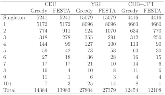
CEU YRI CHB+JPT Greedy FESTA Greedy FESTA Greedy FESTA Singleton 5241 5241 15079 15079 4416 4416 1 5172 5172 8096 8096 4660 4660 2 774 911 924 1070 634 770 3 318 278 355 291 312 250 4 144 99 127 100 113 90 5 59 42 73 53 60 30 6 27 18 36 28 16 15 7 17 17 21 10 14 6 8 16 4 10 8 11 6 9 11 1 6 3 4 4 10+ 7 3 25 14 8 1 Total 14384 13983 27804 27379 12454 12108
Table 2.2: TagSNP distribution on Chromosome 2: Number of tagSNPs per precinct.
Region ENr112 ENr131 ENr113 ENm010 ENm013
No. of SNPs 863 988 1061 539 708
r2 ≥0.5
No. of precincts 55 78 43 44 26
No. of singletons 23 31 16 16 11
No. of tagSNPs (Greedy) 81 110 71 66 41
No. of tagSNPs (FESTA) 75 105 67 61 38
No. of tagSNPs (double cover) 128 183 123 109 67
r2 ≥0.5
No. of precincts 134 184 131 125 72
No. of singletons 63 81 62 61 25
No. of tagSNPs (Greedy) 152 197 142 131 83
No. of tagSNPs (FESTA) 146 193 141 130 81
No. of tagSNPs (double cover) 237 311 229 204 139
Region ENr112 ENr131 ENr113 ENm010 ENm013
# SNPs in dense map 863 988 1061 539 708
# SNPs in sparse map 173 198 213 108 142
One-stage picking
TagSNPs in dense map 75 105 67 61 38
Two-stage picking
Max average r2 85 114 81 72 40
b/w tags and non-tags
Min lowest r2 85 115 80 75 40
b/w tags and non-tags
Min averager2 85 117 82 74 42
among
Other Strategies
Random picking 103.2 137.7 91.4 71.0 52.0
Picket fence 103 136 94 78 52
Use all sparse 200 241 239 134 153
Table 2.4: Comparing different criteria for tagSNP selection: Effect on number of tagSNPs in denser SNP maps
The key improvement of FESTA over the greedy approach is the ‘precinct parti-tioning’ step which enables the exhaustive search to be carried out very rapidly in most of the partitioned precincts. This is similar in spirit to the idea of ‘partition-ligation’ algorithm proposed by Niu et al. [45] for haplotype inference.
Many of the existing tagSNP picking algorithms aim to capture haplotype diver-sity using the reduced set of markers (called haplotype tagging SNPs, htSNPs) such as BEST [25]. They work well when a small number of common haplotypes exist (typically true in the vicinity of a candidate gene) but these approaches often re-quire the knowledge of complete haplotype phase and the boundary of the haplotype blocks. On the other hand, tagSNP selection usingr2 criteria does not require
knowl-edge of block boundaries and can easily be applied to cover the whole chromosome. Multiple-marker tagging strategies [46, 47] in which multiple tagSNPs can be used to represent each untagged SNPs have been proposed. While these methods further
reduce the number of tagSNPs selected, this approach may be sensitive to random genotyping failures.
Our approach is amenable to further computational improvements. For example, parallel programming could be used to search for tagSNPs in separate precincts, fur-ther speeding up the computation.
CHAPTER III
Framework for remapping multiply mapped short
reads
3.1
Introduction
Short read sequencing has been deployed in many areas, such as, cataloging popula-tion variapopula-tion [10], identifying disease susceptibility loci [48], differential gene expres-sion analysis [49, 50] and epigenetics [51, 14].
Most sequencing study designs consist of three main steps, short read sequencing, alignment to the reference sequence and finally downstream analyses. The alignment step is affected by many factors, such as read length, error rate and model, repetitive elements and sequence homology in the reference sequence. These factors, combined with the parameters of the alignment algorithm, can result in the ambiguous align-ment of reads, i.e., these reads can be mapped, with similar confidence, to multiple locations in the reference sequence within the constraints placed on the alignment process.
Several algorithms have been proposed for aligning short sequences to a reference sequence[52, 7, 53]. Most of the alignment algorithms only report reads that can be mapped to a unique location in the reference sequence. As a consequence, themultiply
mapped reads are commonly excluded from downstream analyses. The exclusion of multiply mapped reads can result in information loss leading to decreased sensitivity and specificity in downstream analyses. It can also produce biased results, especially in quantitative analyses [54].
Several methods have been proposed to incorporate multiply mapped reads in down-stream analyses [54, 55]. Most approaches assign multiply mapped reads propor-tionally to their mapping positions, either based on the coverage at the mapping locations[55, 56] or a model based assignment[54, 57]. Many of the approaches were developed specifically for RNA-seq and ChIP-seq datasets. The quantitative nature of the downstream analysis allows for proportional assignment. The proportional assignment approaches cannot be utilized for DNA sequencing projects where down-stream analysis is predicated upon a single accurate alignment of each read.
We present a model based approach designed to identify the most probable map-ping location for the multiply mapped reads. We model the the abundance of the individual bases at each location and use a Gibbs sampler to identify a single most probable mapping for each multiply mapped read. We perform a simulation study to test accuracy in identifying the true alignment of multiply mapped reads using our method. In a subsequent simulation, we use variant discovery as the analysis of interest to quantify the improvement in downstream analysis when adding multiply mapped reads. Our algorithm was able to align upto 87% of correctly mappable short reads back to their true location. The inclusion of multiply mapped reads in variant discovery resulted in a 3% increase in the number of variants detected.
3.2
Methods
LetR be the set of all reads mapped successfully to the reference sequence L. R can be partitioned into two mutually exclusive sets, R1 and R2+, based on the number
of mappings returned by the alignment algorithm. R1 is the set of reads for which
the alignment algorithm found exactly one mapping and R2+ is the set of reads with
multiple mappings.
R1 := {r:r∈R,|Mr|= 1} (3.1)
R2+ := {r:r∈R,|Mr| ≥2} (3.2)
where Mr is the set of mappings for the read r. Each mapping is a location in the
reference sequence to which the read can be aligned.
3.2.1 Count matrix
Consider a single locationi. LetCi ={CiA, CiC, CiG, CiT}be the counts of bases A, C,
G and T aligned to the locationi. Cican be obtained by counting the number of A, C,
G and T bases present in all the reads that contain location iin their alignment, i.e. their selected mapping covers locationi. Conditional on the underlying true genotype at location i, Gi, we assume that the counts follow a multinomial distribution.
(Ci|Gi =g) ∼ M ultinomial(Ni, pg) (3.3) P(Ci|Gi =g) = Ni Ci (pg)Ci = Ni CA i , CiC, CiG, CiT (pAg)CiA(pC g)C C i (pG g)C G i (pT g)C T i (3.4)
where Ni =CiA+CiC +CiG+CiT is the total number of reads covering the location
conditional on the true genotype g.
The probability vector pg depends on the error model for the sequencing process.
In this work, we assume a uniform error model. If the underlying genotype is ho-mozygote, i.e. g = b1/b1, the probability of observing the different bases can be
written as P(o|g = (b1, b1)) = 1−ǫ , o=b1 ǫ 3 , o6=b1 (3.5)
whereǫ is the sequencing error rate per base. In case of a heterozygote genotype, i.e.
g =b1/b2, we can compute the probabilities to be
P(o|g = (b1, b2)) = 0.5− ǫ 3 , o∈ {b1, b2} ǫ 3 , o6∈ {b1, b2} (3.6)
Since the underlying genotype is unobserved, we compute the probability of observing count configuration Ci by integrating over all the possible genotypes.
P(Ci) =
X
g∈{AA,...,T T}
P(Ci|Gi =g)P(Gi =g) (3.7)
We use the reference sequence information to construct the genotype probabilities,
P(Gi). We assume the probability of a base different from the reference sequence
to be 0.001, equal to the expected sequence difference for human sequences. We assign equal probabilities to all three non-reference bases. We use Hardy-Weinberg equilibrium (HWE) to obtain the genotype probabilities. In the absence of reference sequence information, we can assign equal probabilities to all bases and use HWE to get genotype probabilities.
Un-der the assumption that the counts at different locations are independent, we can compute the probability of observing the count matrixC.
P(C) = Y i∈L P(Ci) = Y i∈L X g∈{AA,...,T T} P(Ci|Gi =g)P(Gi =g) (3.8)
Consider a single read r. Let ar be the alignment of read r, i.e. ar is the mapping
selected from Mr as the estimate of the true location of r.
3.2.2 Alignment of uniquely mapped reads
If r ∈ R1, r has exactly one mapping returned by the aligner, i.e. |Mr| = 1. Thus,
there is no ambiguity in the alignment of reads in R1. Let A1 := {ak : k ∈ R1} be
the set of alignments for the reads in R1. We initialize the count matrix using the
sequence of reads in R1 at positions covered byA1.
3.2.3 Alignment of multiply mapped reads
Consider the set of multiply mapped reads, R2+. For each read r ∈ R2+, assume
that a single mapping from Mr has been selected as the current alignment. Let
A2 :={ak :k ∈R2+} be the set of alignments for the multiply mapped reads. Using
Bayes rule, we can write the posterior probability of the alignments in A2 as
P(A2|C, A1) =
P(C|A2, A1)P(A2|A1)
P(C|A1)
(3.9)
We propose a Gibbs Sampling scheme to compute the posterior distribution of the multiply mapped reads. Let r ∈ R2+ be a single multiply mapped read with
map-pings Mr. Additionally, let A2,−r be the set of alignments for all multiply mapped
reads excluding r. We can write the posterior distribution of the alignment, ar, of r
conditional on the current alignment of the other reads.
P(ar =m|C, A2,−r, A1)∝P(C|(A2,−r∪m), A1)P(ar =m|A1, A2,−r) (3.10)
where m is an element of Mr. We assume a uniform prior distribution over the
mappings in Mr, i.e. P(ar =m|A1, A2,−r) =|Mr|−1 ∀m∈Mr. P(ar =m|C, A2,−r, A1) ∝ P(C|(A2,−r∪m), A1) |Mr| (3.11) P(ar =m|C, A2,−r, A1) ∝ P(C|(A2,−r∪m), A1) (3.12)
Since the probability of the count matrix using only the alignments in A2,−r and
A1 is independent of the mappings in Mr, we can simplify the computation of the
conditional distribution as follows
P(ar =m|C, A2,−r, A1)∝
P(C|(A2,−r∪m), A1)
P(C|A2,−r, A1)
(3.13)
Using equation (3.8), we get
P(ar =m|C, A2,−r, A1) ∝ P(C|(A2,−r∪m), A1) P(C|A2,−r, A1) ∝ Y i∈m P(Ci|(A2,−r∪m), A1) P(Ci|A2,−r, A1) (3.14)
We limit our computation to the locations covered by the mapping m. The read contributes one additional count at each location covered by the mapping. Assume that Cr,l is the contribution of the read r to the counts at locationl. As an example,
if the reads contains the base A at location l, Cr,l = (1,0,0,0); if it contains the base
equation (3.8) into (3.14), we get P(ar=m|C, A2,−r, A1) ∝ Y i∈m P(Ci|(A2,−r∪M), A1) P(Cl|A2,−r, A1) ∝ Y i∈m P g∈{AA,...T T} Ni Ci+Cr,i (pg)(Ci+Cr,i) P g∈{AA,...T T} Ni Ci (pg)Ci (3.15)
We iteratively align each multiply mapped read using the conditional distribution derived above. After allowing for burn-in, we sample the alignments of the reads to obtain the joint posterior distribution of the alignments of the multiply mapped reads. We obtain the maximum a posteriori (MAP) estimate of the alignments by selecting the marginal mode of the posterior alignment distribution for each multiply mapped read.
3.2.4 Simulations
We conduct two simulation studies to test the performance of our method. In the first study, we simulate a single individual using the coalescent simulator ms [58]. The population parameters for the coalescent simulation are given in table 3.1. We generate a region approximately the size of chromosome 21. Using the reference sequence of chromosome 21 as the ancestral state, we introduce variants using the sites obtained from the ms haplotypes. We randomly place 70 bp long reads on the simulated chromosomes. Assuming independent errors at each location on the read, we introduce errors using a uniform error model. We generate two datasets, with 10X and 30X average coverages. We use the Burrows-Wheeler aligner, bwa [52], to align these reads back to the reference sequence. Using our algorithm, we obtain the alignment for the multiply mapped reads. We measure the performance of our algorithm using the proportion of multiply mapped reads that were aligned back to their true location in 1000 replicates.
Parameter Value Effective population size (Ne) 10000
Mutation rate (µ) 1.5×10⁻⁸
Recombination rate (r) 1×10⁻⁸
Gene Conversion rate 4.5×10⁻⁹
Table 3.1: Population parameters for simulating short read sequence data
In the second simulation study, we simulate 1Mb long haplotypes for 100 diploid individuals using the same population parameters as the first simulation. We use a 1Mb long sequence from chromosome 1 as the ancestral state. Using the mechanism described above, we generate short reads for each individual with 10X and 30X average coverage. After aligning the short reads using bwa, we use our algorithm to resolve the alignment of the multiply mapped reads. We use glfMultiples [59] to identify single nucleotide variants in the sample. We repeat the variant discovery step using only uniquely mapped reads. We compare the sensitivity and specificity of variant discovery between the two datasets.
3.3
Results
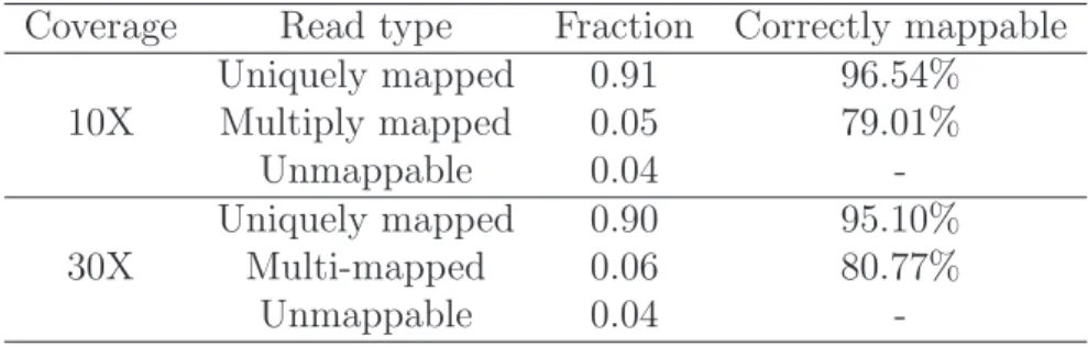
We present the results of our simulation study to characterize multiply mapped reads. Table 3.2 shows the numbers of uniquely mapped and multiply mapped reads with 10 and 30 fold average coverage on chromosome 21. More than 90% of all reads are uniquely mapped to the reference region and 5% of reads are multiply mapped. BWA could not align about 4% of reads. Greater than 95% of the uniquely mapped reads are aligned to their true location in the reference sequence. The proportion of multi-ply mapped reads that contain the true alignment in the list of mappings returned by BWA is approximately 80%. Since 20% of the multiply mapped reads do not contain the true alignment, our algorithm cannot remap them to their true genomic location. Fig. 3.1 shows the proportion of multiply mapped reads aligned to their true genomic
Coverage Read type Fraction Correctly mappable Uniquely mapped 0.91 96.54% 10X Multiply mapped 0.05 79.01% Unmappable 0.04 -Uniquely mapped 0.90 95.10% 30X Multi-mapped 0.06 80.77% Unmappable 0.04
-Table 3.2: Read characteristics for chromosome 21 simulated data
location using the Gibbs sampling approach. The proportion of multiply mapped read aligned correctly increases quickly before plateauing out at 70%. We see a slight in-crease in the proportion of correctly mapped read at 30 fold coverage compared to 10 fold coverage. Since only 80% of multiply mapped reads can be aligned back to their true location, our method is able to align approximately 87% of multiply mapped to their true location conditional on their true mapping being identified by the align-ment algorithm.
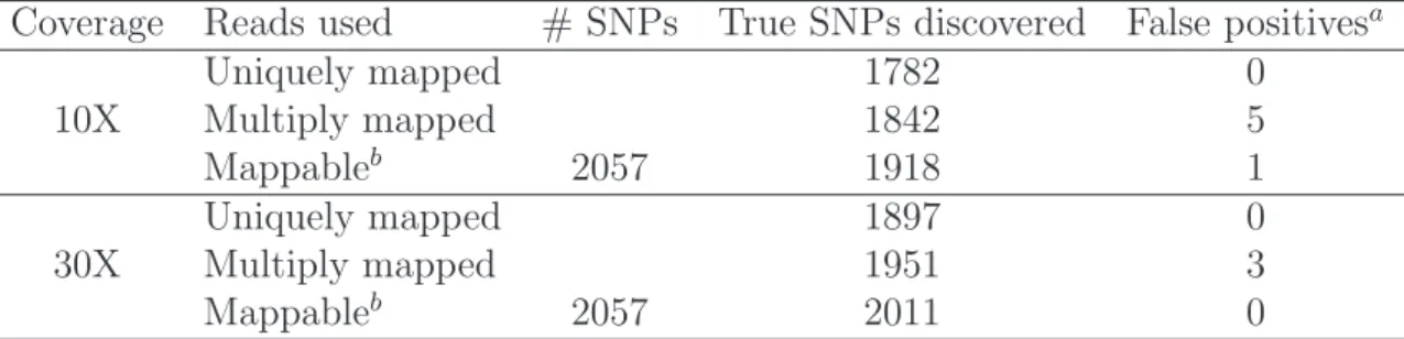
The improvement in variant discovery with the inclusion of multiply mapped reads aligned by our method is given in table 3.3. For the 10 fold coverage data, using only uniquely mapped reads uncovers 87% of all variants present in the sample. Us-ing the alignment provided by our method, we were able to increase the number of variants discovered from 1782 to 1842, a 3% increase. If all multiply mapped reads had been placed in their true genomic location, 93% of all variants would have been discovered. Similar trends can be seen for the dataset with 30 fold average coverage. Variant discovery with uniquely mapped reads resulted in 1897 variants. Including multiply mapped reads in the analysis led to a 3% increase in the number of variants discovered.
Figure 3.1: Proportion of multiply mapped reads aligned to their true location using our algorithm
3.4
Discussion
In this work, we developed a Bayesian framework to identify the true location of multiply mapped reads. In simulation studies, our method was able to resolve the mapping ambiguities of more than 70% of the multiply mapped reads. Restricting to multiply mapped reads which could be correctly assigned, our method was able to correctly align ∼90% of the multiply mapped reads. Incorporating the estimated alignment of multiply mapped reads into variant discovery resulted in a 3% increase
Coverage Reads used # SNPs True SNPs discovered False positivesa Uniquely mapped 1782 0 10X Multiply mapped 1842 5 Mappableb 2057 1918 1 Uniquely mapped 1897 0 30X Multiply mapped 1951 3 Mappableb 2057 2011 0 a
Monomorphic positions identified as single nucleotide variants b
All reads that were mapped by the aligner were assigned to their true location
Table 3.3: Effect of multiply mapped reads on variant discovery
in the number of variants detected.
Since variant discovery is a computationally intensive process, we use the MAP es-timate for downstream analysis. Since ∼20% of the multiply mapped reads are not aligned to their true location, variant calling on a single individual results in a high false discovery rate. Using information from multiple samples helps overcome the adverse effects of misaligned multiply mapped reads.
Most existing methods for resolving multiply mapped reads assign the reads pro-portionally to multiple locations. In contrast, our method can estimate a unique alignment for each multiply mapped read. Further, the Gibbs sampling approach al-lows the estimation of the joint posterior distribution of the alignment of all multiply mapped reads. Using this joint distribution, our method can be used for quantitative analyses by aligning multiply mapped reads proportional to their posterior probabil-ities.
Short read sequencing protocols are constantly evolving, resulting in ever increas-ing read lengths. As read length is inversely proportional to mappincreas-ing ambiguity, this leads to a reduction in the proportion of multiply mapped reads. Paired end
sequenc-ing is another tool that can be used to improve the mappsequenc-ing fidelity. Although these advances result in fewer multiply mapped reads, repetitive sequences, structural vari-ants and sequence homology in the human genome will ensure ambiguity in mapping short read sequences. Our method can be used as an additional tool to extract infor-mation from multiply mapped reads.
CHAPTER IV
Feasibility of admixture mapping to identify rare
susceptibility variants
4.1
Introduction
Genome wide association studies (GWAS)[1] have been the instruments of choice in detecting genetic susceptibility loci. GWAS use genotype-phenotype correlation, com-puted using sets of affected and unaffected samples, to identify loci associated with the trait of interest. GWAS are best suited to detect variants that fall under the Common Disease-Common Variant (CDCV)[60] hypothesis. The CDCV hypothesis proposes that common diseases are caused by commonly occurring genetic variants with low to moderate effect sizes. GWAS have been successfully employed to identify common risk variants for common diseases such as diabetes[2], cardio-vascular diseases[61], Parkinson’s disease [62, 63] and colorectal cancer [64, 65]. They have been used to identify genetic variants affecting quantitative traits such as lipid levels[66, 67] and BMI[68, 69]. While GWAS have been successful in identifying genetic loci influencing many heritable traits [3], in many cases, the variants so identified have not been able to adequately explain the heritability of common diseases [4, 5].
vari-ants that GWAS are not well suited to detect. The Common Disease-Rare Variant (CDRV)[70] hypothesis surmises that the prevalence of common diseases can be at-tributed to the presence of several rare causal variants in the population, each with a moderate to high effect size. The two hypotheses, CDCV and CDRV, reflect the presence of causal variants at different parts of the allelic spectrum of susceptibility variants. These hypotheses fit as complementary pieces in our effort to unravel the underlying genetic architecture of complex common diseases.
Several methods have been proposed to identify rare causal variants [71, 72, 73, 8, 74]. Rare variants mapping methods have been used to find loci affecting LDL cholesterol[12, 75] and HDL cholesterol levels[11]. Since testing each rare variant in-dividually is not statistically powerful, many rare variant mapping methods combine the rare variants across a larger unit, such as a gene or an exon. Subsequently, they test the burden or distribution of rare variants in each testing unit across affected and unaffected samples. Different strategies have been proposed to combine the rare variants across a testing unit, such as the presence or absence or rare variants[11, 7], sum of minor alleles across rare variants[8] and weighted rare allele counts[71].
In admixed populations, i.e. populations with multiple founding populations, we can use the ancestry of a testing unit as one way to collapse information across the variants present in the region. An admixed population derives its ancestry from two or more genetically different founder populations. The chromosomes of individuals from an admixed population consist of a mosaic of genetic material from the different founding populations. A block of shared ancestry is known as an admixture block. Genetic recombination reduces the size of admixture blocks over generations. Figure 4.1 shows the changes in admixed chromosomes over multiple generations.
Admixture mapping is a tool used to identify regions associated with a trait of
Figure 4.1: Admixed chromosomes and admixture blocks
interest by examining the differences in ancestry between affected and unaffected in-dividuals. Consider an admixed population with two founding populations A and B. In the admixed population, the genomic regions that are not associated with the diseases should have ancestry equal to the mixing proportions, irrespective of the dis-ease status of the individuals. For regions associated with the disdis-ease, the ancestry contribution is dependent on the disease status. For affected individuals, we expect to see excess ancestry from the founding population where the region’s contribution to disease prevalence is higher. Conversely, for unaffected individuals, we expect to see diminished ancestry contribution from this founding population. This difference
in ancestry between affected and unaffected samples can be tested to map regions associated with the disease.
Admixture mapping can be used in two flavors. Case-control admixture mapping tests the difference in ancestry between affected and unaffected samples. A more powerful approach is cases only admixture mapping, which compares the ancestry of admixture blocks in cases to the estimated average genome-wide ancestry. Cases only admixture mapping can produce spurious results in the presence of deviations from average ancestry unrelated to the disease.
Admixture mapping has been shown to be powerful in identifying common causal variants [76]. Risk variants for end-stage renal disease[77] have been identified using admixture mapping. Admixture mapping has also yielded promising candidate re-gions associated with prostate cancer. Several diseases including hypertension, lung cancer, stroke have disparate prevalences in African and European populations [78], making them good candidates for admixture mapping. For many of these diseases, susceptibility loci have yet to be identified. Here, we explore the feasibility of admix-ture mapping in the context of mapping rare causal variants.
Data from HapMap [16] and 1000 Genomes[10] projects show that African popu-lations contain more polymorphic sites than European or Asian popupopu-lations. This difference is more pronounced for low frequency and rare variants. Many rare variants are private to one of the two populations and those that occur in both populations seldom have the similar frequencies [10]. This difference in the frequencies of rare variants among populations combined with the CDRV hypothesis, implies a differ-ence in contribution of the locus to disease prevaldiffer-ence in the two populations. Since admixture mapping draws its power from the difference in prevalence contributions,
it is a natural choice to identify loci harboring rare variants.
The first step in admixture mapping is the estimation of the ancestry of admixture blocks. For the remainder of this work, we assume that ancestry of admixture blocks can be accurately estimated. This assumption is justified since modern genome-wide genotyping platforms include a dense set of markers spread across the genome. We can estimate ancestry of genomic locations by combining information from neighboring markers [79, 80]. We compare admixture mapping to single marker association studies using a simulation study. Using a multiplicative model for disease risk, we analyti-cally compute the power of admixture mapping conditional on the contribution of the locus to prevalence in both populations. We simulate the founding populations using
ms[58]. We calibrate the coalescent simulator using a model for population history of Africans and Europeans[81]. We compute the power of the single marker associa-tion tests using simulated cases and controls sampled from the founding populaassocia-tions. The power of the single marker association tests is computed as the proportion of datasets with a significant result using a 1 degree of freedom test for allelic associa-tion. We perform association tests using two strategies, viz., direct association where the causal variants are among the variants tested and indirect association, where a set of tagging SNPs are tested. We compare the performance of admixture mapping to single marker association analysis across different cumulative risk allele frequencies.
Under our simulation settings, we find that admixture mapping has moderate power to detect the susceptibility region. For our disease model, admixed populations with equal contributions from two founding populations yield the best power for admixture mapping. The power of admixture mapping is directly proportional to the cumulative risk allele frequency. When the cumulative risk allele frequency is held under 1% in the European population, admixture mapping has less than 10% power to detect
as-sociation of the region with the disease, even with sample sizes upto 10000 cases and 10000 controls. At a cumulative risk allele frequency of 5% in Europeans, with 10000 cases and controls each, admixture mapping has 60% and 80% power in populations with mixing ratios of 80-20 and 50-50 respectively.
4.2
Methods
In this section, we present the disease model that we use for rare variants. We also derive the relationship between the contribution of the locus to disease prevalence in the founding populations and the admixed populations. Using these results, we ana-lytically compute the power of admixture mapping under the chosen disease model.
We need to set up some parameters to elaborate the disease model and compute the power of admixture mapping. Consider an admixed population, C, with two ge-netically different founding populations. Let the two founding populations be denoted by population A and population B. Let pAand pB = 1−pA denote the contributions
of population A and population B to the admixed population respectively. This im-plies that for any locus not associated with disease, an admixed individual is expected to derive their ancestry from population A with probability pA. Additionally let FA
denote the contribution of the causal region to disease prevalence in population A and let FB be the same in population B. We show that the power of admixture mapping
is a monotonically increasing function of the ratio of the contributions to prevalences.
4.2.1 Disease Model
To compute the power of admixture mapping, we need to specify the underlying disease model. Following the model proposed by Zhu and Risch [82], we assume a multiplicative disease model at each susceptibility locus. In addition, we assume that
the different causal variants at the same locus interact in a multiplicative manner to affect the disease risk.
Consider the causal region in population A. Assume there are K causal variants in this region. We denote the relative risk of causal variant k byrk. Given the
rela-tive risk of all the causal variants and a model of multiplicarela-tive interaction of causal variants, we can write the relative risk associated with a given haplotype h, Rh, as
Rh = K
Y
k=1
rIk(hk) (4.1)
whereI(hk) is a variable indicating whether haplotype hcarries the risk allele at the
k-th causal variant. Given an individual from population A, carrying haplotypes h1
and h2, we can write the risk of disease in that individual as
P(D|(h1, h2), A) = b2Rh1 ·Rh2 = b2 K Y k=1 rI(hk1) k r I(hk 2) k (4.2)
Here, b2 is the baseline risk associated with the null genotypes, i.e. the risk conferred
by carrying no causal variants.
4.2.2 Contribution to prevalence in the founding and admixed popula-tions
Using the haplotype risks, we can compute the contribution of this region to the prevalence of the disease, FA. Let H be the set of all possible haplotypes of the
causal variants. LetfA
write FA in terms of haplotype risks and frequencies as FA = X (h1,h2)∈H∈ P(D|(h1, h2))fhA1f A h2 = X (h1,h2)∈H∈ b2R h1Rh2f A h1f A h2 = X (h1,h2)∈H∈ (bRh1f A h1)(bRh2f A h2) = X h∈H bRhfhA !2 (4.3)
We can derive the contribution of the locus to the prevalence in population B similarly. If we assume that identical haplotypes confer identical risks in both populations, we find that the risk of disease for an individual from population B carrying haplotypes
h1 and h2 is exactly the same as in equation (4.2). Using an approach similar to
equation (4.3), we can compute the contribution of the locus to disease prevalence in population B,FB. FB = X h∈H bRhfhB !2 (4.4)
In the above equation, fB
h is the frequency of haplotypeh in population B. We note
that the difference in contributions to prevalence of the region in the two founding populations is driven by the difference in the frequencies of the haplotypes carrying the causal variants.
We can calculate the contribution to prevalence of the region in the admixed popula-tion by combining the equapopula-tions (4.3) and (4.4). First, we note that for an individual carrying a pair of haplotypes h1 and h2 admixed population, there are three possible
ancestries. They can both trace their ancestry back to a single population, A or B. Alternatively, one haplotype each can be inherited from populations A and B. LetfC h
be the frequency of haplotype h in the admixed population. We can write fC
h as the
weighted mean of the frequencies of the haplotype in populations A and B.
fhC =pAfhA+pBfhB (4.5)
Since we assume that the baseline and haplotype risks remain unchanged in the admixed population, we can explicitly write out the contribution of the region to disease prevalence in the admixed population, FC, as follows
FC = X h1∈H X h2∈H b2Rh1f C h1Rh2f C h2 = X h∈H bRhfhC !2 (4.6)
We can use equations (4.3), (4.4) and (4.5) to simplify equation (4.6).
FC = ( X h∈H bRh pAfhA+pBfhB )2 = ( pA X h∈H bRhfhA+pB X h∈H bRhfhB )2 = npA p FA+pB p FB o2 = p2AFA+p2BFB+ 2pApB p FAFB (4.7)
We can break the contribution to prevalence of the region in the admixed population into three parts.p2
AFA andp2BFB are the contributions from individuals both of whose
haplotypes are inherited from population A and B respectively, while 2pApB
√
FAFBis
the contribution of individuals with one haplotype from each population. Conversely, we can viewFA,FBand√FAFBas the probability of disease given that the individual
is carrying two haplotype from population A, two haplotypes from population B and one haplotype each from either population, respectively.
4.2.3 Power of admixture mapping
We can calculate the power of admixture mapping analytically, conditional on know-ing the contribution of the locus to disease prevalence in the two foundknow-ing populations, viz.,FA andFB. We will focus on case-control admixture mapping. Admixture
map-ping compares the ancestry proportions of cases and controls. It tests the difference in ancestries for cases versus controls using a one degree of freedom χ2 test for
inde-pendence between ancestry and disease status. If the contribution of the region to disease prevalence is the same in both founding populations, the ancestry proportions of cases and controls should be identically distributed and admixture mapping rejects the hypothesis that the region is associated with the disease. Let us consider an admixture mapping setup with nC cases and nC controls sampled from the admixed
population. Let the counts of the 2x2 table be given by nAC,nBC,nAC and nBC.
Ancestry A Ancestry B
Case nAC nBC
Control nAC nBC
Here nAC and nBC are the counts, in cases, of haplotypes inherited form population
A and B respectively. Similarly,nAC andnBC are the counts of haplotypes in controls inherited from population A and B respectively. We can obtain the probability of a haplotype falling in each one of the four cells of the 2x2 table using the contributions of the region to disease prevalence in the founding and the admixed populations. Let P(C, A), P(C, B), P(C, A) and P(C, B) be the aforementioned probabilities. Consider the probability of a haplotype falling in the cell for cases with ancestry in population A.