System size expansion using Feynman rules and diagrams
Philipp Thomas
∗†, Christian Fleck
‡, Ramon Grima
†, Nikola Popovi´
c
∗October 2, 2018
Abstract
Few analytical methods exist for quantitative studies of large fluctuations in stochastic systems. In this article, we develop a simple diagrammatic approach to the Chemical Master Equation that allows us to calculate multi-time correlation functions which are accurate to a any desired order in van Kampen’s system size expansion. Specifically, we present a set ofFeynman rules from which this diagrammatic perturbation expansion can be constructed algo-rithmically. We then apply the methodology to derive in closed form the leading order corrections to the linear noise approximation of the intrinsic noise power spectrum for general biochemical reaction networks. Finally, we illustrate our results by describing noise-induced oscillations in the Brusselator reaction scheme which are not captured by the common linear noise approximation.
1
Introduction
The quantification of intrinsic fluctuations in biochemical networks is becoming increasingly important for the study of living systems, as some of the key molecular players are expressed in low numbers of molecules per cell [1]. The most commonly employed method for investigating this type of cell-to-cell variability is the stochastic simulation algorithm (SSA) [2]. While the SSA allows for the exact sampling of trajectories of discrete intracellular biochemistry, it is computationally expensive, which often prevents one from obtaining statistics for large ranges of the biological parameter space. A widely used approach to overcome these limitations has been the linear noise approximation (LNA) [3, 4, 5].
The LNA is obtained to leading order in van Kampen’s system size expansion [6]. Within this approximation, the average concentrations are given by the solution of the macroscopic rate equations, while the fluctuations about that solution are Gaussian. It is however the case that the LNA can in some instances be in severe disagreement with the solution of the corresponding Chemical Master Equation (CME) which it approximates. One such scenario is encoun-tered in the study of networks that involve bimolecular reactions in which some species are present at low molecule numbers. The system size expansion hence offers the possibility to investigate these discrepancies systematically by taking into account the next order terms that go beyond the LNA. In the past, these higher order terms have been successfully employed in demonstrating deviations of the mean concentrations in stochastic biochemical networks from traditional rate equation models [7, 8], in elucidating the dependence of the coefficients of variation on biochemical network parameters [9], and in estimating two-time correlation functions numerically [10]. Different approaches have also been applied to obtain related estimates analytically in particular cases [11, 12]. In practice, the investigation of these effects is important for inferring biological network parameters and for predicting biochemical dynamics from mathematical models.
A common obstacle for the requisite analysis on the basis of the system size expansion is the increasing algebraic complexity of the resulting equations, as is commonly encountered with higher order perturbation theories. A common remedy is to replace the CME by a truncated partial differential equation that is accurate to some given order in powers of the inverse square root of the system size [6, 13, 14]. For biochemical systems, the latter is given by the reaction volume. In practice, however, the calculation of higher order terms can become cumbersome because of the difficulty involved in solving these differential equations with increasing numbers of terms and relations. In physics, in ∗School of Mathematics and Maxwell Institute for Mathematical Sciences, University of Edinburgh, Edinburgh EH9 3JZ, United Kingdom †School of Biological Sciences, University of Edinburgh, Edinburgh EH9 3JH, United Kingdom
‡Laboratory for Systems and Synthetic Biology, Wageningen University, Netherlands
particular in the theory of elementary particles or statistical fields, powerful techniques that overcome this complexity are Feynman diagrams and the associated rules from which these are constructed [15].
While the construction of path-integrals for master equations is common practice for instance via the Doi-Peliti formalism or similar techniques [16, 17, 18, 19], we build on the functional integral representation introduced by Tirapegui and Calisto [20]. The particular advantage of this formulation is that it enables us to construct a path-integral for the molecular concentrations and, hence, that it facilitates a straightforward system size expansion. Here, we develop the system size expansion of the CME using Feynman diagrams, which allows us to calculate arbitrary multi-time correlation functions to arbitrary order in the (inverse) system size. To that end, we express the expansion of these functions to each order as a finite sum of diagrams. Specifically, we provide a set ofFeynman rulesfrom which the system size expansion can be constructed algorithmically, or simply “drawn” in diagrammatic form. Each of these diagrams is naturally associated with a certain term in the expansion of the correlation functions, and can be evaluated using a simple dictionary. Our methodology hence presents an efficient bookkeeping device for the construction of closed-form expressions from the system size expansion without the need for solving a large number of coupled ordinary differential equations. Its development is the principal aim of the present manuscript.
The methodology is subsequently applied to determine the finite volume corrections to the LNA of the intrinsic noise power spectrum in general biochemical reaction networks. The latter is defined by the Fourier transform of the autocorrelation function. While it is well known that the LNA yields an exact prediction for unimolecular reactions [21], we derive closed-form expressions here for the leading order corrections to these power spectra. The latter are important for the study of networks that include arbitrary bimolecular or complex-elementary reactions. Firstly, we consider reaction networks that are composed of a single species. Secondly, we utilize the eigenvalue decomposition of the Jacobian of the rate equations to derive explicit expressions for the power spectrum in general multi-species networks. We illustrate our results by applying them to a simple network involving bursty protein production and dimerization. Then, we investigate noise-induced oscillations, a phenomenon also known as coherence resonance [22, 23], in the Brusselator reaction scheme. These oscillations are captured neither by the deterministic rate equations nor by the corresponding LNA. In particular, we show that the theory presented here allows us to predict the dynamics of noise-induced oscillations over large ranges of parameters and molecule numbers.
2
The generating functional of the CME
We consider a general reaction network which is confined in some volume Ω, and which involves the interaction ofN distinct chemical species viaRchemical reactions of the type
s1jX1+. . .+sN jXN kj
−→ r1jX1+. . .+rN jXN, (1) wherej is the reaction index running from 1 to R, Xi denotes chemical species i, kj is the reaction rate of thejth reaction, andsij and rij are the stoichiometric coefficients. We denote the probability of observing the molecular population numbersn= (n1, . . . , nN)T at timet, for an ensemble initially prepared in staten0at some previous time
t0, byP(n, t|n0, t0). Under well-mixed conditions, the latter can be shown to satisfy
˙ P(n, t|n0, t0) = Ω R X j=1 N Y i=1 E−Rij i −1 ! ˆ fj n Ω,Ω P(n, t|n0, t0), (2)
which is called the CME [24, 25]. Here, R is the stoichiometric matrix with entriesRij = rij−sij, ˆfj nΩ,Ω
is the microscopic rate function given by the probability per unit time per unit volume for the jth reaction to occur [2], and E−Rij
i is the step operator which is defined by its action on a general function of molecular populations as E−Rij
i g(n1, . . . , ni, . . . , nN) = g(n1, . . . , ni−Rij, . . . , nN) [24]. Note that we underline matrices throughout the manuscript.
2.1
The exact functional integral of the CME
Next, we describe how the generating functional containing the full information of the noise statistics can be expressed as a weighted sum over all possible trajectories of the underlying stochastic process. This representation is often referred to as the path-integral formulation and represents an exact statistic of the process.
We therefore cast the CME, Eq. (2), into the form ˙P(n, t|n0, t0) = ΩL( ˆP,Qˆ)P(n, t|n0, t0) in whichLis a function of the operators ˆ Q= n Ω, Pˆ =−∇ T n, (3) where∇T
n = (∂n1, . . . , ∂nN). By the definition of the step operator Ei, its action on an analytic function g can be
written asQN i=1E
−Rij
i g(n) = e
−(∇TnR )jg(n) = e( ˆPR )jg( ˆQ). Using these definitions, we can express the transition
matrixLas the function
L( ˆP,Qˆ) =X j
e( ˆPR )j−1fˆ
j( ˆQ,Ω). (4)
The above expression is “normally ordered” in the sense that it has all derivatives ˆP to the left and the vector of molecular concentrations ˆQto the right; also, it explicitly depends on Ω. The generating functionalZ(j,j?) for general multi-time moments can then be written as the functional integral proposed by Calisto and Tirapegui [20],
Z(j,j?) = * exp Z t0 t0 dtj?(t) ˆP(t) +jT(t) ˆQ(t) !+ = Z DQDPexp Z t0 t0 dt−ΩPQ˙ + ΩL(P,Q) +jTQ+P j?)δ(Q(t0)−φ0). (5)
An explicit definition of the measure DQDP is provided in Appendix A.1, Eq. (A17), together with a detailed derivation of the above generating functional. Note that the Dirac delta function fixes the deterministic initial condition
Q(t0) =φ0 here. The merit of the functional integral approach lies in replacing the operators ˆQand ˆP with a
real-valued vectorQand a complex-valued vectorP, respectively, which commute. Eq. (5) determines the moments of the CME for all times and can hence be used, at least in principle, to define arbitrary time-correlation functions for the underlying stochastic process.
Even though the functional integral in Eq. (5) is an exact representation of the CME, it does not provide analytical insight into these correlation functions. The reason is that the integration in (5) cannot be carried out analytically in general because Eq. (4) does not represent a quadratic form, which typically prevents one from obtaining exact expressions for the intrinsic noise power spectrum. In the following section, we review a formal diagrammatic definition ofm-point correlation functions; then, we develop simple approximations for these functions on the basis of the system size expansion.
2.2
Correlation functions
We now introduce the exact connected generating functionalW as
W(j,j?) = lnZ(j,j?). (6)
Note that the above definition is convenient computationally, since the first and second cumulants of ˆQare given by the mean concentrations and the centered second moments, respectively. Them-point correlation functions can be defined in both the time and the frequency domain, as follows:
Gm(t1, t2, . . . , tm) = m Y k=1 δj(tk)W(j,j ? ) = Z ∞ −∞ m Y k=1 dωk 2π e iωktk ! "m Y k=1 δj(ωk)W(j,j?) # (j,j?)=(0,0) , (7)
whereδj(t)≡δ/δj(t) is the functional derivative which, augmented byδj(t0)j(t) =δ(t−t0) 1 , follows the usual rules of
differentiation. Analogous definitions apply in the frequency domain representation. With the diagrammatic method in mind we can represent suchm-point functions graphically. For example, the exact one-point function corresponding to the mean concentration may be represented symbolically by a diagram with one external line
ω t
where the blob, which remains to be specified, arises from differentiation of the cumulant generating functionalW. Similarly, the exact two-point function can be represented by
ω1 ω2
t1 t2
(9) Under stationarity, the two-point correlation function only depends on the distance between the two time points. Hence, G2(t1−t2) = δj(t1)δj(t2)W(j,j ? ) (j,j?)=(0,0) = Z ∞ −∞ dω 2πe iω(t1−t2)δ j(ω)δj(−ω)W(j,j ? ), (10)
which implies that the frequency over the whole diagram in Eq. (9) is conserved in the sense thatω=ω1 =−ω2. The
intrinsic noise power spectrum is then defined by the Fourier transform ofG2,
S (ω) =
δj(ω)δj(−ω)W(j,j?)
(j,j?)=(0,0). (11)
General stationarym-point functions can be defined analogously in the Fourier domain, via
Gm(ω1, ω2, . . . , ωm−1) =δ m X k=1 ωk ! "m Y k=1 δj(ωk)W(j,j ? ) # (j,j?)=(0,0) ; (12)
hence, the one-point function in Eq. (8) contributes only at zero frequency, as expected. It is important to note that the derivatives of the cumulant generating functionalW involve only diagrams which are fully connected [26]. Specifically, in the case ofm= 3, the stationary three-point function is represented by
ω1 ω1+ω2 ω2 t1 t3 t2 (13) which concludes the formal diagrammatic representation of thesem-point correlations.
3
System size expansion using Feynman rules
In the limit as Ω→ ∞, the variational principle tells us that the integral in Eq. (5) must be dominated by the minimum of the exponential therein, which is determined from the variational equations
˙ Qα= ∂L ∂Pα =X j e(PR )jR αjfj(Q), ˙ Pα=− ∂L ∂Qα =X j (1−e(PR )j) ∂ ∂Qα fj(Q). (14)
Here, fj(Q) = limΩ→∞fˆj(Q,Ω) denotes the macroscopic rate function. The above equations constitute the exact description of well-mixed reaction networks described by Eq. (1) in the limit of infinite system size. A particular solution of these is given by the macroscopic rate equations
dφ
which is found by lettingP = 0 andQ=φ; the latter represent the saddle point of the functional integral. We now proceed by expanding the exponent in Eq. (5) around that point. The system size expansion is based on the scaling assumption that the fluctuations about the macroscopic stateφdecay as the inverse square root of the system size
Q=φ+ Ω−12q, P = Ω− 1
2p, (16)
which is akin to van Kampen’s ansatz [6, 24]. Note that applying the latter to Eq. (5) provides a local approximation for the generating functional which is valid only in the vicinity of a stable fixed point of Eq. (15). Here, we restrict our analysis to that case. (The above scaling may fail for instance near extinction thresholds or when the macroscopic equations exhibit multistability [27, 28, 18].) We also rescale j = √ΩJ and j? = √ΩJ? correspondingly. The generating functional forq andpis now given by
Z(J,J?) = Z DqDpexp Z t0 t0 dt−pq˙+ (ΩL(Ω−1/2p,φ+ Ω−1/2q)−√Ωpφ˙) +JTq+pJ?δ(q(t0)), (17)
and is related toZ(j,j?) through
Z(j,j?) = exp Z t0 t0 dtφTj ! Z(J,J?). (18)
It remains to expandLin powers of the system size Ω. In order to make this dependence explicit, we expand the microscopic rate functions as
ˆ f(φ,Ω) = ∞ X n=0 Ω−nf(n)(φ), (19)
where the first term is the macroscopic rate functionf(0)(φ)≡f(φ) of the rate equations, Eq. (15). It is important
to note that the form of the above expansion is (i) necessary for the CME to have amacroscopic(deterministic) limit [24], and (ii) that it is implied by the law of mass action derived frommicroscopicconsiderations [25]. The expansion is now obtained along the same lines as in [29], where the system size coefficients have been defined as
D(n)ij..r= X α RiαRjα. . . Rrαfα(n)(φ), J(n)st..zij..r = ∂ ∂φs ∂ ∂φt . . . ∂ ∂φz D(n)ij..r. (20)
Here,D(n)ij..ris the Taylor coefficient of order Ω−nof the jump moments, evaluated at the macroscopic concentrations
φ,J(n)st..zij..r denotes their derivatives, and Rij are the elements of the stoichiometric matrix defined after Eq. (2). In the following we omit the index (n) in the case where n = 0. In particular, Dα equals the right hand side of the macroscopic equations in (15),Jαβ denotes their Jacobian matrix, andDαβ is commonly referred to as the diffusion matrix. Expanding ΩLin terms of Ω−1/2, one obtains
ΩL= ∞ X n=0 ∞ X j=0 Ω−n−21−jL(nj)= Ω 1 2L(0) 0 + Ω 0L(0) 1 +L 0 . (21)
The first term in the above expansion isL(0)0 =pαDα, which equalspφ˙. The next term of order Ω0 is given by the quadratic form
L(0)1 =Jαβpαqβ+ 1
2!Dαβpαpβ, (22)
whereL0
collects all terms that contain inverse powers of Ω. Here, we have adopted Einstein’s summation convention in which repeated Greek indices are summed over. The first few terms ofL0
are given by L0= Ω−12L(1) 0 + Ω −1 2L(0) 2 + Ω −1L(1) 1 + Ω −1L(0) 3 +O(Ω −3 2), (23)
with L(1)0 =pαDα(1), L(1)1 =pαJα(1)βqβ+ 1 2!pαpβD (1) αβ, L(0)2 = 1 2!pαJ βγ α qβqγ+ 1 2!pαpβJ γ αβqγ+ 1 3!pαpβpγDαβγ, L(0)3 = 1 3!pαJ βγδ αβ qβqγqδ+ 1 2! 1 2!pαpβJ γδ αβqγqδ+ 1 3!pαpβpγJ δ αβγqδ+ 1 4!pαpβpγpδDαβγδ. (24) Note that by Eqs. (22) through (24), the expansion ofLin Eq. (21) vanishes for p= 0 to each order in the system size, thus ensuring conservation of probability; see also Appendix A.1. It then follows that in the limit as Ω→ ∞, we can approximate the functional integralZ(J,J?) defined in Eq. (17) by the Gaussian integral
Z0(J,J?) = lim Ω→∞Z(J,J ? ) = Z DqDpexp Z t0 t0 dt −pq˙+pJq+1 2pDp T +JTq+pJ? δ(q(t0)), (25)
which is the LNA and which has also been obtained by Calisto and Tirapegui [20]. Here, the matrix [ J ]αβ =Jαβ is the Jacobian of the macroscopic rate equations, Eq. (15), while D = R diag(f) RT denotes the diffusion matrix. It also follows that Eqs. (23) and (24) determine the leading order correction to the LNA.
Frequency-domain representation of the LNA
Gaussian integrals can generally be evaluated exactly. We perform the integration explicitly in the frequency domain using the Fourier transform. Assuming stationary conditions, the integral will be independent of the initial and the final times, and hence, we can safely taket0→ −∞andt0→ ∞in Eq. (25). The corresponding Fourier transform is
then found from the frequency domain representations
q(t) = ∞ Z −∞ dω 2πe iωt q(ω), p(t) = ∞ Z −∞ dω 2πe iωt p(ω). (26)
Inserting the above expressions into Eq. (25), we have Z0(J,J?) =
Z
DqDpeS0(p,q)δ(q(t
0)), (27)
where the exponentialS0 is given by
S0= ∞ Z −∞ dω 2π −iωp(ω)q(−ω) +p(ω) Jq(−ω) +1 2p(ω) Dp T (−ω) +e−iω0+JT(ω)q(−ω) +p(ω)J?(−ω). (28)
Note that we have included a factor of e−iω0+ here, which accounts for the Ito discretization scheme of the time integral1. The Gaussian integral in Eq. (27) may be performed directly by completing the square in the exponential.
Alternatively, by partial integration, we can utilize the two relations Z DqDp δ δqe S0(p,q) = 0, Z DqDp δ δpe S0(p,q) = 0. (29)
The first relation can be used to derive
δZ0
δJ?(−ω) =J T
(ω) F (ω)Z0, (30)
1The Ito discretization, which has been derived in Appendix A.1, Eq. (A17), has a contribution of P
kδtJTkqk−1 in the exponential.
Inserting Eq. (26) and taking the the limit asδt→0 yieldsR
which, together with the second relation, yields δZ0
δJ(ω) = ( F (ω)J ?
(−ω) + ∆ (ω)J(−ω))Z0, (31)
where have made use of the following two definitions
F (ω) = (iω−J )−1e−iω0+, (32)
∆ (ω) = F (ω) D F†(ω). (33)
The above pair of equations can be integrated to obtain the generating functional of the stationary statistics,
Z0(J,J?) = exp ∞ Z −∞ dω 2π J(ω)TF (ω)J?(−ω) +1 2J T (ω) ∆ (ω)J(−ω) . (34)
Note that we have omitted the explicit dependence on the initial condition here. Note also thatZ0(0,0) = 1 due to
conservation of probability. It may be noted that, for the purposes of calculation, Eqs. (32) and (33) might be written in the eigenbasis of the Jacobian J . It is then clear that F (ω) and ∆ (ω) are well defined only when all eigenvalues of the Jacobian have negative real part, which is the case for a stable fixed point of the macroscopic rate equations, as required by van Kampen’s ansatz; see also the discussion after Eq. (16).
LNA of the power spectra and correlation functions
Using the cumulant generating functional W0 = lnZ0, we now verify that the functional in Eq. (34) agrees with
well-known results obtained from the LNA. The first cumulant is calculated as
hˆq(ω)i0=δJ(ω)W0|(J,J?)=(0,0)= 0. (35)
Hence, it follows from Eq. (16) in combination with the LNA that the average concentrations are well predicted by the macroscopic rate equations. The second cumulant is given by the Fourier transform of the correlation function, as discussed earlier, and evaluates to
hˆq(ω)ˆqT(−ω)i0=δJ(ω)δJ(−ω)W0|(J,J?)=(0,0)= ∆ (ω), (36)
where ∆ (ω) is given by Eq. (33). The above is the well-known result for the spectral matrix, which can be found in [30].
We further haveδJ(ω)δJ?(−ω)W0|(J,J?)=(0,0)= F (ω), which is given by the Green’s function of the linearized rate
equations, as is seen by inverting the Fourier transform of Eq. (32): F (τ) = Z dω 2πe iωτ F (ω) =H(τ−0+)eJτ, (37)
whereH(τ) denotes the Heaviside step-function and we have made use of the fact that (iω−J )−1=R∞
0 dse ( J−iω)s for asymptotically stable J . Note that the factor of e−iω0+in Eq. (32) ensures that the contour of the Fourier integral has to be closed in the lower half of the complex plane on which F (τ= 0) vanishes, thus precluding an instantaneous action of the linear response and, hence, implementing causality. Similarly, the expression for ∆ in the time domain, ∆ (τ) =R dω
2πe
iωτ∆ (ω), can been obtained from
∆ (τ) = F (τ)σ+ σFT(−τ), (38)
where ∆ (0) = σ is just the covariance matrix ofq[30]. This relation between the size of fluctuations ∆ (τ) and the linear response function F (τ), or equivalently its frequency domain representation, Eq. (33), is commonly obtained in dynamic perturbation theories of equilibrium and non-equilibrium steady states and referred to as thegeneralized fluctuation-dissipation theorem [31, 19].
3.1
Setting up the perturbation expansion
Next, we make use of a well-known trick [15] to express the exact generating functional in terms of the Gaussian integralZ0, Eq. (25). For any analytic functionf(ˆp,qˆ), the Gaussian expectation value can be written as
hf(ˆp(t),ˆq(t0))i0=
Z
DqDpf(p(t),q(t0))eS0(p,q)
=f(δJ(t), δJ?(t0))Z0, (39)
where we have used Eq. (27). We thus define the function
K(p,q) = exp Z ∞
−∞
dtL0(p,q), (40)
and note that, using Eq. (39), the exact generating functional can be expressed as Z(J,J?) =K(δJ?, δJ)Z0(J,J?) = e
R
dtL0(δJ?(t),δJ(t))Z
0(J,J?). (41)
Analogous expressions are common to dynamical perturbation theories [15, 26]. The above expression represents an ideal starting point for the purposes of detailed calculation, since the exponential therein can be expanded in powers of the inverse square root of the system size. Using Eq. (23) in Eq. (40), we find that, in the frequency domain,
K(δJ?, δJ) = exp X0Z ∞ −∞ n Y k=1 dωk 2π ! δ n X k=1 ωk ! Ω−(n2+j−1)L(j) n (δJ?, δJ), (42)
where the summationP0is over all valuesn >0,j≥0 satisfyingn+ 2j >0. This result can in principle be used to evaluate expectation values explicitly to any order in the system size expansion.
3.2
Use of diagrams for explicit calculation
In order to illustrate the utility of Feynman diagrams for the evaluation of expectation values, we exemplify here the calculation of the mean concentrations up to order Ω−1. The analysis is carried out in parallel both analytically and using the diagrammatic method. (Readers familiar with the technique can safely skip this section.) We therefore expand hqˆii= δJi(ω)Z (J,J?)=(0,0) = Ω−12δ(ω)δJ i(ω)Z0(J,J ? ) (J,J?)=(0,0) + Ω−12δ(ω) Z ∞ −∞ 3 Y k=1 d`k 2π ! δ 3 X k=1 `k ! Jαβγ δJ? α(`1)δJβ(`2)δJγ(`3)δJi(ω)Z0(J,J ? ) (J,J?)=(0,0) + Ω−12δ(ω) Z ∞ −∞ 3 Y k=1 d`k 2π ! δ 3 X k=1 `k ! Jαβγ δJ? α(`1)δJβ?(`2)δJγ(`3)δJi(ω)Z0(J,J ? ) (J,J?)=(0,0) + Ω−12δ(ω) Z ∞ −∞ d` 2π δ(`)D(1)α δJ? α(`)δJi(ω)Z0(J,J ? ) (J,J?)=(0,0) + Ω−12δ(ω) Z ∞ −∞ 3 Y k=1 d`k 2π ! δ 3 X k=1 `k ! Dαβγ δJ? α(`1)δJβ?(`2)δJγ?(`3)δJi(ω)Z0(J,J ? ) (J,J?)=(0,0) +O(Ω−1) (43) Since δJi(ω)Z0(J,J ?)
(J,J?)=(0,0)= 0, we are left with four integrals. These integrals can be evaluated analytically
from the identities
δJ(ω)δJ(ω0)Z0(J,J?) (J,J?)=(0,0)=δ(ω+ω 0 ) ∆ (ω), δJ?(ω)δJ(ω0)Z0(J,J?) (J,J?)=(0,0)=δ(ω+ω 0 ) F (ω), δJ?(ω)δJ?(ω0)Z0(J,J?) (J,J?)=(0,0)= 0, (44)
in combination with Wick’s theorem [26, 32], which states that the expectation value of a Gaussian distribution is given by the sum over all possible products of pairs:
δX1(ω1). . . δX2n(ωn)Z0 (J,J?)=(0,0)= X pairings δXi1δXi2Z0 (J,J?)=(0,0). . . δXim−1δXimZ0 (J,J?)=(0,0). (45)
There is, however, a simpler way which is based on a representation of these integrals in diagrammatic form. We begin by assigning the line to ∆ (ω) and the line to F (ω), while denoting the matricesJβγ
α ,J γ αβ, Dαβγ by . The second term in Eq. (43) thus becomes
δ(ω) Z ∞ −∞ 3 Y k=1 d`k 2π ! δ 3 X k=1 `k ! Jαβγ δJ? α(`1)δJβ(`2)δJγ(`3)δJi(ω)Z0(J,J ? ) =δ(ω)[ F (ω)]iα 1 2!J βγ α Z d` 2π[ ∆ (`)]βγ +δ(ω)[ ∆ (ω)]iα 2 2!J βγ α Z d` 2π[ F (`)]βγ . =1 2! i ω J ` βγ α + 2 2! i ω J ` βγ α | {z } =0 (46)
where we adopt the convention that`, being internal, has to be integrated out. Note that the second term appears twice due to the symmetryJβγ
α =Jαγβ, but that the latter vanishes because R d`
2πF (`) = 0, by Eq. (37). The absence of closed loops in the linear response is thus a consequence of causality.
Similarly, we have δ(ω) Z ∞ −∞ 3 Y k=1 d`k 2π ! δ 3 X k=1 `k ! Jαβγ δJ? α(`1)δJβ?(`2)δJγ(`3)δJi(ω)Z0(J,J ? ) = 2 2! i ω ` Jαβγ + 1 2! i ω ` Jαβγ = 0 (47) and δ(ω) Z ∞ −∞ d` 2π δ(`)D(1)α δJ? α(`)δJi(ω)Z0(J,J ? ) =−Ω−12J−1 iαD (1) α = ω i Dα(1) (48)
where we have introduced an extra vertex forD(1)α which attaches only one external line. Combining Eq. (43) with Eqs. (46) through (48), we find that, up to order Ω−1/2,hqˆ
iiis then simply the sum of the following two diagrams:
hqˆi(ω)i= Ω −1 2 1 2! i ω J ` βγ α + ω i Dα(1) +O(Ω−1). (49)
These diagrams are known as tadpoles, and lead to the corrections to the mean concentrations predicted by the rate equations. Note that the above sum of diagrams differs from a pure loop expansion by the second diagram, the reason being the explicit dependence of the microscopic rate functions on the system size Ω. In the following, we denote these extra vertices, more specifically those withn6= 0 in Eq. (20), by . Noting, moreover, that the closed loop above corresponds to σ =R d` 2π∆ (`), we can write hqˆii=−Ω −1 2J−1 iα 1 2!J βγ α σβγ+D(1)α ≡Ω−12 i. (50)
We may now conclude that the average concentration is given by Dni Ω E =φ− 1 ΩJ −1 iα 1 2!J βγ α σβγ+D(1)α +O(Ω−2), (51)
to order Ω−1. The same result has been obtained from EMREs (Effective Mesoscopic Rate Equations) by Grima
[7] for the case of purely elementary reactions, albeit on the basis of a truncation of the partial differential equation underlying van Kampen’s system size expansion to order Ω−1/2. As we have seen above, the direct computation of
these corrections can be quite involved. In the next section, we summarize a set of rules, commonly known as Feynman rules, which greatly simplify the required calculations to a merely combinatorial task, and which hence eliminate the need to invoke Wick’s theorem directly.
3.3
The Feynman rules for the correlation functions
The above observations can be summarized by the following set of rules:
(i) To calculate them-point cumulant correlation function, drawmlines (called external lines). (ii) Pick a number of symbols either fromDi1..in,J
...in
i1... orD
(s)
i1..in,J
(s)...in
i1... . Denote the former by , and the latter
by . A symbol withnindices is represented by ann-vertex (a node in which exactlynlines meet).
(iii) Leave one end of each external line free and attach the other end to a vertex index. Draw lines between the remaining vertex indices such that the diagram is connected.
(iv) For each external line account with a factor of Ω−1/2, for each vertexD
i1..in orJ
...in
i1... account with a factor of
Ω−(n−2)/2, and for each vertexDi(1s)..inorJ
(s)...in
i1... account with a factor of Ω
−s−(n−2)/2
. The order in the system size expansion to which the diagram contributes is the product of these factors.
(v) Repeat steps (i)-(iv) and draw all possible diagrams up to the desired order in the system size expansion. (vi) To each line that connects two upper vertex indices, assign a propagator . To each line that connects
an upper and a lower vertex index, assign a propagator . Note that there are no lines connecting two lower vertex indices.
(vii) Assign to external lines attached to an lower vertex index, and otherwise .
(viii) Assign a frequency to each line, and conserve frequency at each vertex. Conserve also total frequency over the entire diagram.
(ix) The value of each diagram is given by the product of the factors associated with all lines and vertices. To each line with frequencyω, assign the factor ∆ (ω). To each line with frequencyω, assign the factor F (ω).
(x) A diagram with L internal loops will have L internal frequencies that are not fixed by the requirement for frequency conservation. Integrate over all frequencies, with measure d`i/(2π).
(xi) Sum over all internal indices, accounting for the symmetry properties of the given diagram. The corresponding symmetry factor equals the number of ways in which the vertices in a diagram can be connected, divided by the symmetry of the vertex factors. The latter is given bynu!nd!, since the vertex factorJ
j1...jnu
i1...ind is invariant against
permutation of all upper or lower indices.
(xii) In conclusion, them-point correlation function equals the sum over all connected diagrams withmexternal lines.
4
Corrections to the LNA of the power spectra
We now demonstrate the diagrammatic technique by evaluating the power spectrum to order Ω−2, i.e., including the next term beyond the LNA, which is important for reaction networks involving bimolecular reactions. The calculation of the requisite corrections is greatly facilitated by the set of Feynman rules presented in the previous section. The power spectrum is simply obtained as the sum of all diagrams with two external lines that include products of vertices of order Ω−2. It is clear from Eqs. (23) and (24) that, to this order, we only need to consider diagrams with at most
two vertices.
Since the system size expansion involves non-zero corrections to the mean concentrations, as derived in Section 3.2, it is important to ensure that the expressions for the power spectrum of fluctuations are indeed centered around the
(a) (b)
(c) (d)
(e)
Figure 1: Construction of two-point diagrams. Distinct topologies of two-point diagrams contributing to the intrinsic noise power spectrum to order Ω−2. Since each external line contributes a factor of Ω−1/2 we only need to consider diagrams comprising a single vertex of order Ω−1or combinations of two vertices which each contribute a factor of Ω−1/2. Note that the system size expansion involves diagrams (b) and (d) that differ from a pure loop expansion.
corrected mean concentrations. Note that the generating functionals for the centered concentration fluctuations ( ˆQ− hQˆi) and the deviations from the rate equations ˆq, Eq. (41), are related by the exponential factor eΩ1/2R
dt0J(t0)hq(t0)i . Thus, it follows that the sequence of cumulants generated by their logarithms agrees beyond the first one, and, hence, that these generate an equivalent series of connected diagrams which is used in the following.
In order to simplify the construction of these diagrams, we divide them into the three basic topologies shown in Figs. 1(a) and (b), which are denoted as tadpoles; Figs. 1(c) and (d), which we denote as snails, but which are also referred to as tadpoles in the literature; and Fig. 1(e), which are denoted as loop diagrams, respectively. We have already encountered tadpoles in Section 3.2. Denoting the contribution from tadpole diagrams byT, the contribution from snail diagrams byS, and the contribution from loop diagrams byL, we can express the spectral matrix S as
S (ω) = 1 Ω∆(ω) + 1 Ω2T(ω) + 1 Ω2S(ω) + 1 Ω2L(ω) +O(Ω −3 ); (52)
here, the last two terms determine the power spectrum to order Ω−2. We now outline the explicit evaluation, in turn, of these diagrams.
4.1
Tadpoles, and all that. . .
In Fig. 2, we list all possible diagrams stemming from tadpoles. These contain one subdiagram which has already been evaluated in Section 3.2. The sum of the diagrams in (a) and (b) is then given by
T1(ω) = 1 2! Jσδρ Jαβγ + 1 2! D(1)α Jαβγ + h.c. = 1 2! Fiα(ω)Jαβγ γF † βj(ω) + h.c. (53)
Note that, by including also the Hermitian conjugate (h.c.) of the above diagram, we have accounted for the contribu-tion from an equivalent time-reversed diagram. Note also thatγis defined by Eq. (50). Analogously, for the diagrams in Figs. 2(c) and (d), we find
Jσδρ Jαβγ (a)S= 1 D(1)α Jαβγ (b)S= 1 Jδρ σ Jβγ α (c)S= 1 D(1)α Jβγ α (d)S= 1
Figure 2: Tadpole diagrams. All tadpole diagrams contributing to order Ω−2 to the intrinsic noise power spectrum. Note that none of these have internal symmetries; hence, the symmetry factor isS = 1 throughout.
T2(ω) = 1 2! Jσδρ Jβγ α + 1 2! D(1)α Jβγ α + h.c. = 1 2! Fiα(ω)Jαβγγ∆βj(ω) + h.c. (54)
Finally, we denote the sum over the diagrams shown in Fig. 2 by
T(ω) =T1(ω) +T2(ω). (55)
4.2
About snails. . .
The next topology, Fig. 1(c), contains only a 4-single vertex where two upper indices are contracted in a loop. We have already found that such a loop equals the correlation matrix σ. The resulting diagrams are given in Figs. 3(a) and (b), implying S1(ω) = 2 2!2! Fiα(ω)JαβγδσγδFβj† (ω) + h.c., (56) S2(ω) = 3 3! Fiα(ω)Jαβγδσγδ∆ † βj(ω) + h.c. (57)
Note that the diagram in Fig. 3(b) is non-zero only when one considers reactions with non-elementary propensity functions, e.g., trimolecular reactions or those of Michaelis-Menten type [33].
We progress to the topology shown in Fig. 1(d), which is resolved by a simple matrix multiplication. The two possible diagrams are generated from 2-vertices, as shown in Figs. 3 (c) and (d). The result is
S3(ω) =Fiα(ω)Jα(1)β∆ † βj(ω) + h.c., (58) S4(ω) = 1 2!Fiα(ω)D (1) αβF † βj(ω) + h.c., (59)
We denote the sum over all these diagrams by
S(ω) =
4
X
n=1
Sn(ω), (60)
Jαβγδ (a)S= 2 Jβγδ α (b)S= 3 Jα(1)β (c)S= 1 D(1)αβ (d)S= 1
Figure 3: Snail diagrams: All snail diagrams contributing to order Ω−2 to the intrinsic noise power spectrum. The symmetry factors (S) follow by considering the ways in which the right external line can be attached to the corresponding vertex. Jαβγ Dδρσ (a)S= 3! Jαβγ Jδρσ (b)S= 2 Jαβγ Jδσρ (c)S= 4 Jαβγ Jδρσ (d)S= 4 Jαβγ Jδσ ρ (e)S= 1
Figure 4: Loop diagrams. All diagrams that contribute to order Ω−2 to the intrinsic noise power spectrum, and that contain a frequency loop integral. The symmetry factors (S) follow by considering the ways in the right external line can be attached to the corresponding vertex, times the permutations of all internal lines. Note that in (e), we have only accounted for half of these permutations, since the diagram is self-adjoint.
4.3
Concerning loop diagrams
The evaluation of all diagrams considered thus far has been possible by simple matrix multiplication. However, to evaluate the diagrams in the topology in Fig. 1(d), namely those which contain a loop formed by connecting two 3-vertices, one has to calculate explicitly the integrals occurring therein. The relevant diagrams are listed in Fig. 4, all of which consist of a line F connected to the 3-vertexJαβγ, and are hence non-zero only for networks involving bimolecular reactions. We can then write the overall contribution from each diagram in the general form
Ln(ω) = 1 2Fiα(ω)J βγ α h Vj(n)(ω) i βγ+ h.c., (61)
where we have defined the vertex functions Vj(n)(ω), which are effectively 3-tensors. As we shall see, the latter consist of a 3-vertex with the frequency loop integrated out.
Evaluation of vertex functions
Let us study in detail the vertex function Vj(1)(ω) that is defined by the right hand side of the first diagram shown in Fig. 4(e). The latter is simply the diagram with the vertexJαβγremoved, and can be written as
h Vj(1)(ω)i βγ≡ 3×2 3! ω ` ω+` j γ β Dρδσ = Z ∞ −∞ d` 2πFβρ(ω+`) DρδσF † σj(ω) Fδγ†(`), (62)
where the symmetry factor has been obtained via the considerations in the caption of Fig. 4. We now evaluate the integral by inserting the Fourier transform of F (ω), Eq. (37), into the above equation to show that its solution can be obtained by solving a linear matrix equation. We start by fixing the external indexjand write down the 3-vertex matrix with the frequency loop integrated out:
Vj(1)(ω) = Z ∞ −∞ d` 2πF (ω+`) M j (1)(ω) F † (`) = Z ∞ 0 dτe( J−iω)τMj(1)(ω)eJTτ, (63)
where we have set [ Mj(1)]ρδ = DρδσFσj† (ω). As is shown in Appendix A.2, one can verify that, in this form, V j
(1)
satisfies Sylvester’s matrix equation
SVj(1)= Mj(1)(ω), (64)
whereS represents the linear operator
S(•)≡( J−iω)(•) + (•) JT. (65)
It is useful to define also the adjoint ofS through
(•)S†≡( J +iω)(•) + (•) JT. (66)
Sum of loop diagrams
The vertex functions corresponding to the diagrams shown in Figs. 4(b) through (d) can be evaluated in an analogous fashion, as demonstrated in Appendix A.3, and are given by
h SVj(1)i βγ =DβγσF † σj(ω), h SVj(2)i βγ =Jβγδ ∆δj(ω), h SVj(3)i βγ= 2J γ βσF † σj(ω), h SVj(4)i βγ = 2σβρJγρδ∆δj(ω), (67)
which includes the result of the previous section. The evaluation of the remaining vertex functions shown in Fig. 4(e), however, results in two sets of equations
h SVj(5) i βγ= 1 2σβρJ ρδ σ F † σj(ω)σδγ, h S†Vj(6)i βγ =1 2J βγ σ F † σj(ω), (68)
that also involve the adjoint of S defined by Eq. (66), as derived explicitly in Appendix A.3. The sum of the five diagrams in Fig. 4 is then given by
L(ω) = 5 X n=1 Ln(ω) = 1 2Fiα(ω)J βγ α h Vj(ω)i βγ + h.c., (69) where Vj(ω) =P5 n=1 V j (n)(ω) + σV j
(6)(ω)σ. In the following, we present explicit solutions to these equations for
4.4
Explicit solution for one molecular species
We consider the case of chemical reactions involving only a single species, in which the expressions derived in the previous section can readily be solved in closed form. For brevity, we setD=D11,J=J11,D(1)=D
(1) 11,J
(1)=J1(1) 1 ,
D3=D111, and=1. The power spectrum to order Ω−2 is then given by a sum of four contributions,
S(ω) = 1 Ω∆(ω) + 1 Ω2T(ω) + 1 Ω2S(ω) + 1 Ω2L(ω) +O(Ω −3 ). (70)
The first term is simply the contribution from the LNA, which evaluates to ∆(ω) = D
J2+ω2. (71)
The second term is given by
T(ω) = J2+ω2 D0+J0 J D J2+ω2 , (72)
while the third reads
S(ω) = 1 J2+ω2 D(1)+D00σ+ (2J(1)+J00σ) J D J2+ω2 . (73)
The remaining term is obtained by solving Eqs. (67) and (68) usingS−1
= (2J−iω)−1, and substituting the result in Eq. (69). We find L(ω) = 1 J2+ω2 J0 (2J)2+ω2 D(2J2−ω2)D 0 + 2σJ0 J2+ω2 + 2J(2D 0 +D3+σ2J0) , (74)
which concludes our derivation. In Appendix A.4 we have verified the agreement of the above result with a particular case discussed by Calisto and Tirapegui [20].
4.5
Explicit solution for general multi-species reaction networks
General expressions for the higher order corrections can be obtained via the diagonalization of the Jacobian J of the macroscopic rate equations, which satisfies
U J U−1= diag(λ1, . . . , λN). (75)
Here, the matrix on the right hand side is diagonal, withλ1, . . . , λN the eigenvalues of J . The spectral matrix S can then be transformed as ˜ S (ω) = U S (ω) UT= 1 Ω ˜ ∆ (ω) + 1 Ω2T˜(ω) + 1 Ω2˜S(ω) + 1 Ω2L˜(ω) +O(Ω −3 ). (76)
Applying the LNA, we find explicitly ˜ ∆ij(ω) = ˜ Dij (λi−iω)(λj+iω) , (77)
where the coefficient is obtained from the transformed diffusion matrix ˜D . The general transformation rules for the system size coefficients, Eq. (20), are given by
˜
D(ij..rn) =UiαUjβ. . . UrρD
(n)
αβ..ρ, ˜
J(n)st..zij..r = (UiαUjβ. . . Urρ)(U −1 σsU −1 τ t . . . U −1 ζz)J (n)στ..ζ αβ..ρ. (78)
In order to evaluate these, we transform ˜S= USUT such that for any ˜V = U V UT, we have [ ˜S ˜V ]ij= (λi+λj− iω)[ ˜V ]ij,and, hence,
[ ˜V ]ij= 1 λi+λj−iω
Using Eqs. (53) through (56) and (58), we find ˜ Tij(ω) = 1 2 δiαδjβ (λi−iω)(λj+iω) ˜ Jαβγ + ˜Jαµγ δµνD˜νβ λν−iω ˜ γ+ (ω→ −ω, α↔β) (80) and ˜ Sij(ω) = 1 2 δiαδjβ (λi−iω)(λj+iω) ˜ D(1)αβ+ ˜Jαβγδσ˜γδ+ (2 ˜J(1) µ α+ ˜J µγδ α σ˜γδ) δµνD˜νβ λν−iω + (ω→ −ω, α↔β). (81)
Further, solving Eq. (67) and (68) using Eq. (79) and substituting the result in Eq. (69), we deduce ˜ Lij(ω) = 1 2 δiαδjβ (λi−iω)(λj+iω) ˜ Jθζ α δµθδγζ λµ+λγ−iω × ( ˜Jµγδ + 2˜σµρJ˜γρδ)δδl ˜ Dlβ λl−iω + 2 ˜Jµβγ + ˜Dµγβ+ ˜σµρJ˜βρδσ˜δγ + (ω→ −ω, α↔β), (82)
where we have used the symmetry of the last summand in the angled brackets in Eq. (82). Note also that these equations are to be summed over all Greek indices, according to our summation convention.
From the analytical form of these correction terms, we recover the well-known fact that they vanish for reaction networks with at most unimolecular reactions; see for instance [21]. Note that the microscopic rate functions in Eq. (19) are at most linear in the concentrations, and independent of the system size Ω, in that case. The former observation shows that all vertices with multiple upper indices are identically zero, while the latter implies that ˜D(1)αβ and ˜J(1)µ
α vanish and, hence, that the corrections given by Eqs. (81) and (82) are absent. It also follows from Eq. (50) that (80) vanishes, as the mean concentrations predicted by the CME agree to this order with the prediction from the rate equations. These correction terms hence stem from the nonlinearity in the law of mass action, and thus must increase with the size of the rate constants in the bimolecular reactions.
It can also be deduced from Eqs. (80) through (82) that the nonlinear corrections to the power spectrum involve denominators (λi−iω)(λj+iω) and, hence, that they contribute to the amplitude of the power spectrum at the frequencies of the linear relaxation modes. Further, Eq. (82) involves the denominatorλµ+λγ−iωwhich stems from nonlinear relaxation modes that are not described by the linear response. These additional frequencies appear in the sums of pairs of the eigenvalues of the linear relaxation modes. Such corrections are particularly important when close to bifurcation points; for example, in the case of noise-induced oscillations below a Hopf bifurcation point, they lead to a secondary harmonic, and a zero-frequency component in the power spectrum. This phenomenon has been reported by some of the authors in [12], where the Chemical Langevin Equation was used, and is derived here explicitly from the CME for the first time.
5
Applications
5.1
Dimerization
As a first example, we consider bursty expression of a protein and dimerization. Bursty synthesis may arise through the finite lifetimes of the associated transcripts [34]. A simple reaction system describing synthesis in bursts of sizem can be formulated as
∅−−→kin mX, 2X−→1 ∅ (83) The expansion coefficients can be calculated from the stoichiometric matrix S = (m,−2) and the microscopic rate functions, which are given by the series
ˆ f(n,Ω) =fn Ω + 1 Ωf (1)n Ω (84) with f(φ) = (kin, φ2)T and f(1)(φ) = (0,−φ)T, from which one deduces J = −4φ and D = 2(2 +m)φ2. The
concentration predicted by the macroscopic rate equation, Eq. (15), is obtained asφ= (mkin/2)1/2. Hence, the power
spectrum and variance, as found from the LNA, reads ∆(ω) = 2(2 +m)φ
2
16φ2+ω2 , σ=
2 +m
Further, usingJ0=−4 andD(1)=−4φthe mean concentration is calculated from Eq. (51) as Dn Ω E =φ+ 1 Ω 2−m 8 +O(Ω −2 ). (86)
The higher order correction to the intrinsic noise power spectrum can now be derived by substituting the coefficients J00= 0, D0 = 4(2 +m)φ, D00 = 4(2 +m) J(1) = 2, andD3 = 2 m2−4
φ2 into Eqs. (85), (72) and (74), and by making use of Eq. (70). The result is
S(ω) = 1 Ω∆(ω) + Ω 2 " 64(2 +m)φ3 2(2 +m)φ2−(m−1)ω2 (16φ2+ω2)2(64φ2+ω2) # . (87)
Finally, the Fourier transform of the above expression yields the autocorrelation function n(t+τ) Ω − Dn Ω E n(t) Ω − Dn Ω E = Z dω 2πe iωτ S(ω) = e−4φτ σ Ω+ 1 Ω2 (2 +m) 96 (14−13m+ 12(3m−2)τ φ) + 1 Ω2 (2 +m) 96 e −8φτ (11m−10) +O(Ω−3). (88)
The first term includes a Ω−2correction to the amplitude of the linear response, while the second represents additional
relaxation terms that decay twice as fast; see also the discussion concluding Section 4.5.
In order to verify the accuracy of our analysis, we calculate the Ω−2 correction to the variance given by the LNA
using Eq. (25) together with Eqs. (28) through (30) from [13]: * n(t) Ω − Dn Ω E2 + = 1 Ωσ+ 1 Ω2 (2 +m)(2−m) 48 +O(Ω −3 ), (89)
which agrees with Eq. (88) when evaluated atτ = 0. The particular case ofm= 2, which obeys detailed balance with a Poissonian steady state, has been considered by Chaturvedi and Gardiner [11] (withκ2= 2 in their notation). They
obtained the autocorrelation function 1 Ωe −4φτ σ+ 1 Ω2 e−8τ φ 1 + e4τ φ(4τ φ−1) 2 +O(Ω −3 ), (90)
which agrees with Eq. (88) in this case. It is interesting to observe that, despite the detailed balance of the reactions, the nonlinearity in the law of mass action manifests itself in the non-trivial dependence of the Ω−2 terms.
5.2
Noise-induced oscillations in the Brusselator reaction
The Brusselator describes a commonly studied set of autocatalytic oscillatory reactions [35], which involve two species interacting via ∅ k0 −* )− k1 X, X−→b Y, 2X+Y −→a 3X. (91)
The form of the propensities Ω ˆf(n,Ω) = (Ωk0, k1nX, bnX, anYnX(nX −1)Ω−2) implies the following expansion of the rate functions, Eq. (19),
ˆ f(n,Ω) =fn Ω + 1 Ωf (1)n Ω , (92)
where f(φ) = (k0, k1[X], b[X], a[Y][X]2) and f(1)(φ) = (0,0,0,−a[Y][X]). This expansion, together with the
stoi-chiometry R = 1 1 −1 1 0 0 1 −1 , (93)
determines the system size coefficients, Eq. (20). Specifically, the solution of the macroscopic rate equations, Eq. (15), is given by [X] = k0
k1 and [Y] =
bk1
ak0. The Jacobian of these equations then reads
J = b−k1 a[X]2 −b −a[X]2 . (94)
i iii iv ii v 0 2 4 6 8 0 1 2 3 4 a b A B C 0.5 1 1.5 2 2.5 3 3.5 0 0.1 0.2 0.3 0.4 0.5 0.6 0.7 Ω S( ω ) frequency (ω/2π) Ω=10 Ω=25 Ω=50 Ω=100 LNA 0.5 1 1.5 2 2.5 3 3.5 0 0.1 0.2 0.3 0.4 0.5 0.6 0.7 po w er s pe ct ru m Ω=10 Ω=25 Ω=50 Ω=200 LNA frequency (ω/2π) Ω S( ω )
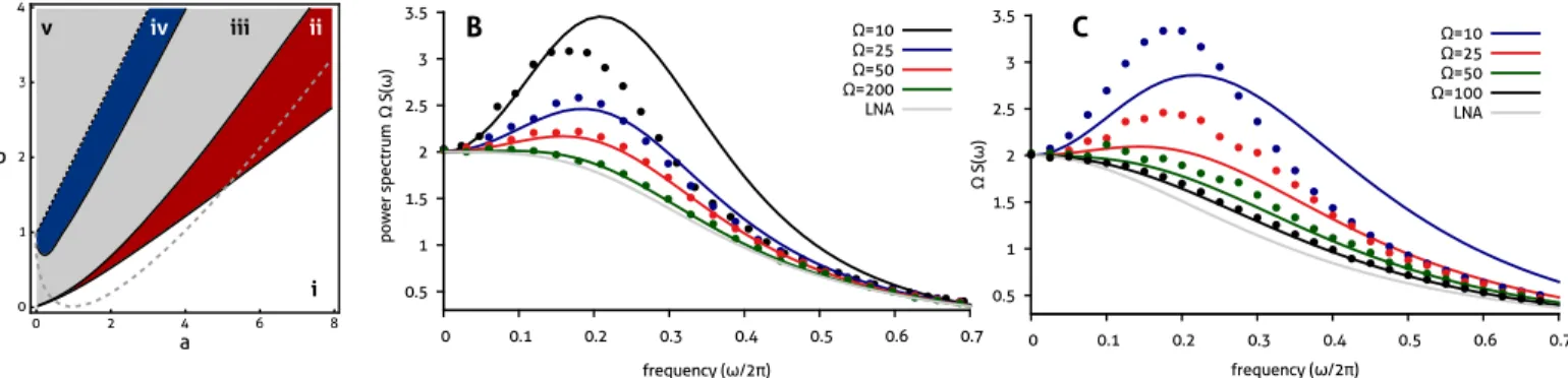
Figure 5: Noise-induced oscillations in the Brusselator reaction: (A) Comparison of the parametric dependence of noise-induced oscillations for speciesX with the prediction from the LNA and with that obtained by including higher order corrections in the system size expansion, for Ω = 20. In region (i, white area), both theories predict that no oscillations will occur; in (ii, red), the higher order expansion predicts noise-induced oscillations which are missed by the LNA. Note that these oscillations appear both for deterministically stable nodes and foci (separated by a dashed gray line). In regions (iii, gray) and (iv, blue), both theories predict noise-induced oscillations. Region (iv, blue) includes the appearance of secondary harmonics that are not captured by the LNA close to the deterministic Hopf bifurcation (dashed black line). The deterministically oscillatory regime in (v, gray) is not described by either theory. (B) The intrinsic noise power spectrum in the case of a deterministic focus (k0 = 1 =k1, a= 4.5,b = 2) is shown for decreasing values of Ω. For large Ω, the monotonous dependence on frequency is captured by the LNA (dashed gray line). A decrease in volume reveals noise-induced oscillations that are well described by the Ω−2 corrections (blue and red lines), but not by the LNA. These predictions are verified by stochastic simulation (dotted). Reducing the volume to Ω = 10, we observe that our theory only qualitatively accounts for the frequency dependence. (C) A similar dependence is observed in the parameter regime corresponding to a deterministic node (k0 = 1 = k1, a= 7.5, b = 3). However, for small volumes, the higher order expansion only yields a qualitative description for the power spectrum of the noise-induced oscillations. (Note that in (A) and (B), the spectrum has been multiplied by Ω such that the prediction from the LNA is the same for all system sizes.)
Using Eq. (51), the mean concentrations are obtained as DnX Ω E = [X] +O(Ω−2), DnY Ω E = [Y] + 1 Ω 2b 2a[X]2−b a[X]2(a[X]2+k 1−b) +O(Ω−2), (95)
which are accurate to order Ω−1. Hence, to this order, the prediction from the CME agrees with the one from the macroscopic rate equations for speciesX, but not for speciesY. The leading order corrections to the power spectrum can be derived either algebraically or by making use of the eigenvalue representation, as follows. The eigenvalues of the Jacobian in Eq. (94) are given by
λ1,2=− 1 2 a[X] 2 +k1−b ±1 2 q (a[X]2+k 1−b)2−4ak0[X], (96)
while the corresponding eigenvectors areUi1 =b, and Ui2 = (λi+k1−b), fori = 1,2. In particular, we see that
the deterministic system undergoes a Hopf bifurcation when the real part of the above eigenvalues becomes positive. Since, strictly speaking, the system size expansion only applies to monostable systems, we requireb < a[X]2+k1. The
resulting analytical expressions for the power spectrum are, however, rather involved. Hence, we restrict our analysis to the study of speciesX in the case wherek0 = 1 =k1. On the basis of the LNA, we obtain
∆X(ω) =
2 a2+ (b+ 1)ω2
The intrinsic noise power spectrum, including corrections of orderO(Ω−2), is then obtained via the procedure derived in Section 4 and reads
SX(ω) = 1 Ω∆X(ω) + 1 Ω2 P5 i=1aiω2i A(ω) +O(Ω −3 ), (98)
where the denominator is given by
A(ω) =(a−b+ 1) (a−b+ 1)2+ω2 × a2+ω2 (a−b)2−2b+ 1 +ω42 16a2+ 4ω2 (a−b)2−2b+ 1 +ω4 . (99) Here, the coefficientsai are defined as
a1=32a4b −3(11a+ 9)b3+ ((58a+ 75)a+ 42)b2−(((49a+ 96)a+ 72)a+ 19)b+ 4((a+ 3)(4a+ 3)a+ 3)a+ 8b4
, a2=8a2b 16a6+ 36a5(3−2b) + 4a4((34b−69)b+ 17)
+a3((2(121−72b)b−359)b+ 40) +a2(3b(b((32b−37)b+ 131)−12)−172) +2a(b(((10(3−2b)b−133)b+ 88)b+ 63)−18) + (b−1)2(((8b−7)b+ 82)b+ 1)b , a3=8b 12a7+a6(8−40b) +a5 32b2−58b+ 3 +a4 37b3+ 128b2+b−55 +a3(63−2b((b(44b+ 59)−52)b+ 24)) +a2 b b 70b2+ 34b−189 b+ 228 −159 −52 −4a(b−1)2(((7b−4)(b+ 2)b+ 3)b+ 3) + 5(b−1)4(b+ 1)2b , a4=8b −a5+ 3a4(b−1) +a3(14−b(4b+ 5)) +a2(b(b(7b+ 59)−75)−17) +a(((42−b(9b+ 35))b+ 21)b+ 17) + 4 b2−12 b, a5=−8b a3+a2(7b+ 1)−a(7(b+ 1)b+ 5) + (b+ 1)2b. (100)
The above explicit expression for the power spectrum can be used to quantify the periodicity of typical trajectories of the underlying stochastic process, which is for instance of importance in the study of single-cell oscillations [36]. Specifically, if the deterministic stability is given by a stable fixed point, a peak in the intrinsic noise power spectrum indicates a noise-induced oscillation. The parametric dependence of these oscillations is analyzed in Fig. 5 using Eq. (98) for a system size of Ω = 20. We find that the LNA predicts the fluctuations to decay monotonically with increasing frequency in parameter regions (i) and (ii), while it postulates noise-induced oscillations in parameter regions (iii) and (iv). By contrast, taking into account higher order corrections as given by the second term in Eq. (98), we infer that the dynamics is also oscillatory in region (ii), which is at odds with the prediction from the LNA. In Figs. 5B and C, we verify this dependence in two parameter regimes, one in which the eigenvalues of the Jacobian, as given in Eq. (96), are complex, and another in which these eigenvalues are purely real, corresponding to stable node oscillations [37]. There, we also show the dependence of the oscillations on the system size Ω. Finally, we note that our theory predicts the presence of secondary harmonics in the vicinity of the Hopf bifurcation (dashed black) that cannot be described by the LNA. An approximate treatment that accounts quantitatively for these effects has been given by some of the authors elsewhere [12].
6
Discussion
In this article, we have presented a general diagrammatic approach for the systematic evaluation of multi-time cor-relation functions from the system size expansion that goes beyond the common LNA. As we have demonstrated, application of the proposed set of Feynman rules allows for the calculation of higher order corrections in the expansion to be performed in an algorithmic fashion. In brief, our methodology permits the representation of the corresponding correlation functions by a sum of diagrams which can be truncated to the desired order in the inverse system size. Each diagram is itself derived from a set of Feynman rules and can be readily translated into certain integrals in the frequency domain. The technique therefore represents an effective bookkeeping device for the purposes of detailed calculation on the basis of the system size expansion.
We emphasize that our approximation for the generating functional does not exceed the accuracy provided by the LNA, from which correlation functions are ultimately generated. Renormalization theory typically employs the Legendre transform of the cumulant generating functional for that purpose; the latter can be constructed either from a diagrammatic expansion of the associated correlation functions, or of the vertex functions alone [15, 19, 26].
Different diagrammatic methods have been applied to obtain stochastic perturbation series using the Doi-Peliti coherent state path-integral in homogeneous or spatial models of population dynamics [16, 28, 32, 19]. The nonlinear
reactions are therein treated as a perturbation to a functional of non-interacting, or “free”, species. In the present perturbative ansatz, however, the Gaussian functional Z0 takes the role of a “free theory” which arises from the
exact generating functional via the LNA in the limit of large system size, i.e., via a linearization of the concentration fluctuations about the macroscopic limit of the full interacting reaction network. As we have demonstrated, our methodology is significantly simpler than present techniques for the system size expansion [13, 38, 10, 12] that are equivalent, but that rely instead on the explicit solution of high-dimensional systems of ordinary differential equations. In particular, it does not involve the calculation of higher moments. Similar perturbation expansions may as well be obtained, for instance, through the functional integral of the Doi-Peliti approach or the Poisson representation [17]. Our choice of the equivalent Calisto-Tirapegui path-integral enjoys the particular advantage that the form of the expansion is in one-to-one correspondence with the system size expansion, as originally proposed by van Kampen.
We have demonstrated the resolution of the diagrammatic expansion to order Ω−2 by deriving closed-form expres-sions for the intrinsic power spectra of general biochemical networks. The resulting expresexpres-sions are more accurate than the ones obtained from the common LNA. We have illustrated the utility of our approach through the analytical computation of the autocorrelation function in a dimerization reaction and through a study of noise-induced oscilla-tions in the Brusselator reaction. Specifically, we have demonstrated that our approach allows for the identification of noise-induced oscillations in parameter regimes that are not captured by the conventional LNA, including in regimes in which a deterministic stability analysis predicts either stable foci or nodes. These discrepancies are of particular interest for the analysis of single cell rhythms that are sustained by noise due to low number of molecules [36, 37, 12]. Our approach may hence serve to deepen our understanding of stochastic dynamics in biochemical networks.
Acknowledgments
We thank Claudia Cianci and Pierce Munnelly for interesting discussions. RG gratefully acknowledges support from SULSA (Scottish Universities Life Sciences Alliance).
A
Appendix
A.1
The functional integral representation
Here, we derive the functional integral representation of the CME ∂
∂tP(n, t|n 0
, t0) = ΩL(−∇n,n)P(n, t|n0, t0), (A1)
wheren denotes theN-dimensional state vector and the operatorL(−∇n,n) = Pj(e(−∇
TR ) j −1) ˆf
j nΩ,Ω
is the transition matrix of the the CME, Eq. (2), that is “normally ordered” in the sense that it has all derivatives∇n to the left and allnto the right.
Operator formulation of the CME
In a first step, we determine a set of eigenfunctions for the following two operators ˆ
Q≡ n
Ω, ˆ
P ≡ −∇Tn, (A2)
which satisfy the commutation relation [ ˆQ,Pˆ] = Ω−11 . The normal ordering ofLsuggests that a suitably chosen set will satisfy the eigenvalue equations ˆQ|Qi=Q|Qi and hP|Pˆ =hP|P. Using the identity e−Ω ˆP QQˆeΩ ˆP Q= ˆQ+Q
[39] together with ˆQ|0i= 0, we verify that
|Qi ≡ |Q0i ⊕ |Q1i ⊕. . .|QNi= exp(Ω ˆP Q)|0i, (A3)
is an eigenvector of ˆQwith eigenvalueQ. Defining
hP|= Z
we verify that the above is an eigenvector of ˆP with eigenvalueP. Likewise, we have hQ|= ΩN Z dP 2πie −ΩP Q hP|, (A5)
where the domain ofP is the imaginary axis such that hQ|Q0i = δ(Q−Q0). Note also that these states are not orthogonal, as
hP|Qi= eΩP Q, hQ|Pi= e−ΩP Q. (A6)
The partition of unity can be derived as
1 = ΩN Z dQdP 2πi e −ΩP Q| QihP|, (A7)
which follows from ΩN Z dQdP 2πi e −ΩP Q |QihP|= ΩN Z dQ Z d ˆQ0 Z d ˜P 2πe iΩ ˜P(Q0−Q) |QihQ0| = Z dQ Z dQ0δ(Q0−Q)|QihQ0| = Z dQ|QihQ|. (A8)
Here, we have changed the integration variable viaP →iP˜ in the first line. Similarly, we find 1 = ΩNR dP
2πi|PihP|. We now associate an abstract state vector|Ψ(t)isuch thathQ|Ψ(t)i=P(Q, t) is the probability density function to observe the concentrationsQat timet. Using the resolution of unity, Eq. (A7), we can write
|Ψ(t)i= Z
dQ|QiP(Q, t). (A9)
Multiplying Eq. (A1) with|Qiand integrating over allQ, we find that|Ψisatisfies the evolution equation ∂
∂t|Ψi= ΩL( ˆP, ˆ
Q)|Ψi. (A10)
The above result is exactly equivalent to the Fock space representation of Doi-Peliti [16, 18, 19], which uses creation-annihilation operators defined bya†i|ni=|n1, . . . , ni+ 1, . . . , nNi andai|ni=ni|n1, . . . , ni−1, . . . , nNi, as well as the Cole-Hopf transformationa†i = ePˆi and a
i = e
ˆ
PiΩ ˆQ
i such thata †
iai = Ω ˆQi [18]. For our purposes, the present parametrization of ˆQ and ˆP is, however, preferable, since it enables us to construct the functional integral for the molecular concentrations ˆQin a straightforward fashion.
Note also that by multiplying Eq. (A10) with the eigenstateh0|=R
dQhQ|belonging toP = 0, we must have ∂
∂t Z
dQP(Q, t) = Ωh0|L(0,Qˆ)|Ψi= 0.! (A11)
Hence, we requireL(0,Qˆ) = 0 by conservation of probability, which is ensured by the definition of L given after Eq. (A1).
Path-integral formulation of the transition probability
The solution of Eq. (A10) for an ensemble initially prepared in state|Q0iat timet0is given by|Ψ(t)i= eΩL(t−t0)|Q0
i. Hence, the transition probabilityhQ|Ψ(t)ireads
P(Q, t|Q0, t0) =hQ|eΩL(t−t0)|Q0i = ΩN Z dP 2πie −ΩP Qh P|eΩL(t−t0)|Q0i. (A12) Note that in the second line, we have made use of the relation in (A7). We continue by slicing the time evolution from t0totintoL−1 pieces with a time step ofδt= (t−t0)/L, inserting Eq. (A7)L−1 times into the above expression:
hP|eΩL(t−t0)|Q0i= L−1 Y k=1 ΩN Z dQkdPk 2πi e −ΩPkQk ! hP|eδtΩL|QL−1ihPL−1|eδtΩ L |QL−2i. . .hP1|eδtΩ L |Q0i. (A13)
SinceL( ˆP,Qˆ) is normally ordered, we have
hPk|L( ˆP,Qˆ)|Qk−1i=L(Pk,Qk−1)hPk|Qk−1i. (A14)
The time-sliced transitions can then be evaluated in the limit asL→ ∞when the time stepδtbecomes infinitesimally small, as follows: hPk|eδtL|Qk−1i=hPk|Qk−1i+δthPk|ΩL( ˆP,Qˆ)|Qk−1i+O(δt 2 ) ≈exp ΩPkQk−1+δtΩL(Pk,Qk−1) , (A15)
which is correct up toO(δt2). Substituting back into Eq. (A12), we find
P(Q, t|Q0, t0) = ΩN lim L→∞ L−1 Y k=1 Z dQk ! L Y k=0 Z dP k 2πi ! exp " − L X k=0 ΩPk(Qk−Qk−1)−δtΩL(Pk,Qk−1) # , (A16)
which expresses the transition probability as a sum over paths of the stochastic process. Note that the factor ΩN is the Jacobian determinant relatingP(Q, t|Q0, t0) andP(n, t|n0, t0) Note also that the endpoints are not contained in the integration range here.
Functional integral representation
In order to calculate the generating functional given by Eq. (5) in the main text, we replace the transition matrix in Eq. (A16) by ΩL → ΩL+ ˆP j?+jTQˆ. Then, we multiply the transition probability by the initial condition δ(Q(t0)−φ(t0)), and integrate out the remaining state vectors. The result is the generating functional
Z(j,j?) = lim L→∞ L Y k=0 ΩN Z dQkdPk 2πi ! × expδt L X k=0 −ΩPk (Qk−Qk−1) δt + ΩL(Pk,Qk−1) +Pkj?+jTQk−1 δ(Q(t0)−φ(t0)) ≡ Z DPDQexp Z t t0 dt−ΩPQ˙ + ΩL(P,Q) +P j?+jTQδ(Q(t0)−φ(t0)), (A17)
where the measureDPDQdenotes the integral obtained by the limiting process in Eq. (A17).
A.2
Sylvester matrix equation
We consider the following Fourier integral V(ω) =
Z ∞
0
dτe( J−iω)τM (ω)eJTτ, (A18)
which determines the vertex matrices defined in Eq. (63), recall Section 4.3. Applying the linear operatorS(ω)(•) = ( J−iω)(•) + (•) JT to the above equation, we find
S(ω)V(ω) = Z∞ 0 dτ(∂τe( J−iω)τ) M eJ Tτ + Z ∞ 0 dτe( J−iω)τM (∂τeJ Tτ ). (A19)
By partial integration, we then obtain
S(ω)V(ω) + M (ω) = 0. (A20)
As a special case, we considerω= 0, from which it follows that the integral
σ = Z ∞
0
dτeJτBBTeJTτ (A21)
is a general solution to the Lyapunov equation
A.3
Explicit evaluation of vertex functions
The result of the previous subsection can be applied to evaluate the vertex functions defined in Section 4.3, as follows. Considering first h Vj(3)(ω)i βγ≡ 2×2 2! ω ` ω+` j γ β Jδσρ = 2 Z ∞ −∞ d` 2πFβδ(ω+`) Jδσρ Fσj† (ω)∆ργ(`) (A23) and setting [ Mj(3)]δρ= 2Jδσρ F † σj(ω), we find Vj(3)(ω) = Z ∞ −∞ d` 2πF (ω+`) M j (3)(ω) ∆ (`) = Z ∞ −∞ dτ e−iωτF (τ) Mj(3)(ω) ∆T(τ) = Z ∞ 0 dτ e( J−iω)τMj(3)(ω)σ eJTτ, (A24) thus, S(ω)Vj(3)(ω) + Mj(3)(ω)σ = 0. (A25)
Next, consider the vertex
h Vj(∗)(ω)i βγ≡ 1 2! ω ` ω+` j γ β Jσρδ =1 2 Z ∞ −∞ d` 2π∆βρ(ω+`) JσρδF † σj(ω) ∆δγ(`). (A26)
This can be written as the sum of two contributions, letting [ Mj(5)]δρ= (1/2)JσρδF † σj(ω), we have Vj(∗)(ω) = Z ∞ −∞ d` 2π∆ (ω+`) M j (5)(ω) ∆ (`) = Z ∞ −∞ dτ e−iωτ∆ (τ) Mj(5)(ω) ∆T(τ) = Z ∞ 0 dτ e( J−iω)τσMj(5)(ω)σ eJTτ +σ Z ∞ 0 dτ e( J−iω)†τMj(5)(ω)eJτ σ ≡ Vj(5)(ω) + σVj(6)(ω)σ , (A27)
thus, the quantities Vj(5)and Vj(6)satisfy
S(ω)Vj(5)(ω) + σMj(5)(ω)σ = 0,
Vj(6)(ω)S†(ω) + Mj(5)(ω) = 0. (A28)
A.4
Van Kampen’s example
The first example in which higher order corrections were probed using the system size expansion was given by van Kampen [6]. He considered the creation and annihilation of electron-hole pairs in a semiconductor following the kinetic scheme
∅ kin
in the case wherem= 1. The stoichiometry of these reactions and their associated propensities are given by R = (m,−1) andfˆ= (kin, φ2)T, respectively. The LNA yields
∆(ω) = 2(2 +m)φ
2
16φ2+ω2 , (A30)
while the correction to the mean concentration predicted by the macroscopic rate equations is given by =− 1
Ω1/2
m+ 1
8 . (A31)
The intrinsic noise power spectrum can then be expressed using Eq. (70) together with Eqs. (71), (72) and (74):
S(ω) = 1 Ω∆(ω) + 1 Ω2 " 4(1 +m)φ3 (1 +m)φ2−(2m−1)ω2 (4φ2+ω2)2(16φ2+ω2) # +O(Ω−3). (A32)
The particular case of m = 1 has been studied by van Kampen [24], and has later been corrected by Calisto and Tirapegui [20]. The Fourier transform of the Ω−2term in the square brackets yields the correction to the autocorrelation function 1 Ω φ 4e −2φτ + 1 Ω2 e−4τ φ+ e−2τ φ(2τ φ−1) 8 +O(Ω −3 ), (A33)
which agrees with the result given in [20].
References
[1] McAdams H and Arkin A 1997Proc Natl Acad Sci USA94814–819 [2] Gillespie D 2007Annu Rev Phys Chem 5835–55
[3] Elf J and Ehrenberg M 2003Genome Res132475–2484 [4] Hayot F and Jayaprakash C 2004Phys Biol 1205 [5] Paulsson J 2005Phys Life Rev 2157–175
[6] Van Kampen N 1976Adv Chem Phys 34245–309 [7] Grima R 2010J Chem Phys 133035101
[8] Ramaswamy R, Gonz´alez-Segredo N, Sbalzarini I F and Grima R 2012Nat Commun3779 [9] Thomas P, Matuschek H and Grima R 2013BMC Genomics 14S5
[10] Scott M 2012IET Syst Biol 6116–124
[11] Chaturvedi S and Gardiner C 1978J Stat Phys 18501–522 ISSN 0022-4715
[12] Thomas P, Straube A, Timmer J, Fleck C and Grima R 2013J Theor Biol 335222–234 [13] Grima R, Thomas P and Straube A 2011J Chem Phys 135084103
[14] Grima R 2011Phys Rev E 84056109
[15] Srednicki M 2007Quantum field theory(Cambridge University Press) [16] Peliti L 1985J Phys (Paris)461469–1483
[17] Droz M and McKane A 1994J Phys A: Math Gen27L467
[18] Kamenev A 2011Field theory of non-equilibrium systems (Cambridge University Press)
[19] T¨auber U 2014Critical dynamics: a field theory approach to equilibrium and non-equilibrium scaling behavior
(Cambridge University Press)
[20] Calisto H and Tirapegui E 1993J Stat Phys 71683–703 ISSN 0022-4715 [21] Warren P, T˘anase-Nicola S and Ten Wolde P 2006J Chem Phys 125144904
[22] Ushakov O, W¨unsche H J, Henneberger F, Khovanov I, Schimansky-Geier L and Zaks M 2005Phys Rev Lett95 123903
[23] McKane A, Nagy J, Newman T and Stefanini M 2007J Stat Phys 128165–191
[24] van Kampen N 1992Stochastic processes in physics and chemistry (North Holland) ISBN 0444893490 [25] Gillespie D 1992Physica A188404–425
[26] Zinn-Justin J 2002Quantum Field Theory and Critical Phenomena(Clarendon Press) ISBN 9780198509233 [27] Hanggi P, Grabert H, Talkner P and Thomas H 1984Phys Rev A29371
[28] Moloney N and Dickman R 2006Braz J Phys 361238–1249 [29] Thomas P, Matuschek H and Grima R 2012PloS one7e38518
[30] Gardiner C 2009Stochastic methods: a handbook for the natural and social sciences (Springer) [31] Keizer J 1987Statistical thermodynamics of nonequilibrium processes (Springer)
[32] T¨auber U 2012J Phys A: Math Theor45405002
[33] Thomas P, Straube A and Grima R 2011J Chem Phys 135181103 [34] Shahrezaei V and Swain P 2008Proc Natl Acad Sci 10517256–17261 [35] Prigogine I and Lefever R 1968J Chem Phys 48
[36] Westermark P, Welsh D, Okamura H and Herzel H 2009PLoS Comput Biol 5e1000580 [37] Toner D and Grima R 2013J Chem Phys 138055101
[38] Cianci C, Di Patti F, Fanelli D and Barletti L 2012Eur Phys J Spec Top 2125–22
[39] Orszag M 2008Quantum optics: including noise reduction, trapped ions, quantum trajectories, and decoherence