Boston University
OpenBU http://open.bu.edu
Economics BU Open Access Articles
2019
Testing jointly for structural
changes in the error variance and
coefficients of a linear regress...
This work was made openly accessible by BU Faculty. Please share how this access benefits you. Your story matters.
Version First author draft
Citation (published version): Pierre Perron, Yohei Yamamoto, Jing Zhou. 2019. "Testing jointly for structural changes in the error variance and coefficients of a linear regression model." Unpublished Manuscript, Department of
Economics, Boston University. https://hdl.handle.net/2144/40070
Testing jointly for structural changes in the error
variance and coe¢ cients of a linear regression model
Pierre Perrony Boston University
Yohei Yamamotoz Hitotsubashi University Jing Zhoux
Seeking Sense Investment Management Co., Ltd. April 16, 2019; revised October 21, 2019
Abstract
We provide a comprehensive treatment for the problem of testing jointly for struc-tural changes in both the regression coe¢ cients and the variance of the errors in a single equation system involving stationary regressors. Our framework is quite general in that we allow for general mixing-type regressors and the assumptions on the errors are quite mild. Their distribution can be non-normal and conditional heteroskedastic-ity is permitted. Extensions to the case with serially correlated errors are also treated. We provide the required tools to address the following testing problems, among others: a) testing for given numbers of changes in regression coe¢ cients and variance of the errors; b) testing for some unknown number of changes within some pre-speci…ed max-imum; c) testing for changes in variance (regression coe¢ cients) allowing for a given number of changes in the regression coe¢ cients (variance); d) a sequential procedure to estimate the number of changes present. These testing problems are important for practical applications as witnessed by interests in macroeconomics and …nance where documenting structural changes in the variability of shocks to simple autoregressions or Vector Autoregressive Models has been a concern.
JEL Classi…cation: C22;Keywords: Change-point; Variance shift; Conditional
heteroskedasticity; Likelihood ratio tests.
Perron acknowledges …nancial support from the National Science Foundation under Grant SES-0649350. We are grateful to Zhongjun Qu for comments and for pointing out an error in a previous draft.
yDepartment of Economics, Boston University, 270 Bay State Rd., Boston, MA, 02215 ([email protected]). zDepartment of Economics, Hitotsubashi University, 2-1 Naka Kunitachi, Tokyo, 186-8601 Japan ([email protected]).
xSeeking Sense (Shanghai) Investment Management Co., Ltd., Taiping Finance Tower, 488 Middle Yincheng Road, Shanghai, China 200120 ([email protected])
1 Introduction
Both the statistics and econometrics literature contain a vast amount of work on issues re-lated to structural changes with unknown break dates, most of it designed for a single change (for an extensive review, see Perron, 2006 and Casini and Perron, 2019b). The problem of multiple structural changes has received attention mostly in the context of a single regres-sion. Bai and Perron (1998, 2003a) provide a comprehensive treatment of various issues: consistency of estimates of the break dates, tests for structural changes, con…dence inter-vals for the break dates, methods to select the number of breaks and e¢ cient algorithms to compute the estimates; see also Hawkins (1976). Perron and Qu (2006) extend this analysis to the case where arbitrary linear restrictions are imposed on the coe¢ cients of the model. Also, Kurozumi and Tuvaandorj (2011) propose an information criterion for the selection of the number of changes; see also Liu, Wu and Zidek (1997). Bai, Lumsdaine and Stock (1998) consider asymptotically valid inference for the estimate of a single break date in multivariate time series allowing stationary or integrated regressors as well as trends with estimation carried using a quasi maximum likelihood (QML) procedure. Also, Bai (2000) considers a segmented stationary VAR model estimated again by QML when the break can occur in the parameters of the conditional mean, the variance of the error term or both. Kejriwal and Perron (2008, 2010) deal with issues related to testing and inference with multiple structural changes in a single equation cointegrated model. Perron and Yamamoto (2014) derive the limit distribution of the estimates of the break dates in models with endogenous regressors estimated via an instrumental variable method, while they argue in Perron and Yamamoto (2015) that using standard least-squares methods is preferable both for estimation and test-ing. Casini and Perron (2019a) provides a limit distribution of the least-squares estimate of the break date in a linear model based on a continuous-time asymptotic framework, which delivers substantial improvements with respect to inference using the concept of highest density regions, i.e., con…dence intervals with adequate coverage rates and smaller average lengths, especially for small breaks.
With respect to testing for changes in the variance of the regression error, the results are quite sparse. Horváth (1993) considers a change in the mean and variance (occurring at the same time) of a sequence of i.i.d. random variables with moments corresponding to those of a normal distribution. Davis, Huang, and Yao (1995) extend the analysis to an autoregressive process under similar conditions. Aue et. al. (2009) propose non-parametric tests for changes in the variances or autocovariances of multivariate linear or non-linear time series
models. Deng and Perron (2008) extended the CUSUM of squares (or CUSQ) test of Brown, Durbin and Evans (1975) allowing general conditions on the regressors and the errors (as suggested by Inclán and Tiao, 1994, for normally distributed time series). Xu (2013) provides a further extension with a robust estimate of the long-run variance of the squared errors of closer relevance to our objectives. Andrews (1993) considers a one-time structural change under a Generalized Method of Moment (GMM) setting, thereby allowing for changes in both coe¢ cients and variance though occurring at the same date; see McConnell and Perez-Quiros (2000) for a related application. Qu and Perron (2007a) consider a multivariate system estimated by quasi maximum likelihood which provides methods to estimate models with structural changes in both the regression coe¢ cients and the covariance matrix of the errors. They provide a limit distribution theory for inference about the break dates and also consider testing for multiple structural changes, though restricted to normally distributed errors and breaks in coe¢ cients and variance occurring at di¤erent dates.
We build on Qu and Perron (2007a) to provide a comprehensive treatment of testing jointly for structural changes in both the regression coe¢ cients and the variance of the errors in a single equation involving stationary regressors, allowing the break dates to be di¤erent or overlap. Our framework is general and allows for general mixing-type regressors. The assumptions on the errors are mild; their distribution can be non-normal and conditional heteroskedasticity is permitted. Extensions to the case with serially correlated errors are also treated. We provide the required tools to address the following testing problems, among others: a) testing for given numbers of changes in regression coe¢ cients and variance of the errors; b) testing for some unknown number of changes within some pre-speci…ed maximum; c) testing for changes in variance (regression coe¢ cients) allowing for a given number of changes in the regression coe¢ cients (variance); d) sequential procedures to estimate the number of changes present. Note that we adopt a QML approach instead of one based on GMM. Either could be used in principle. The main advantage of using the QML approach based on normal errors is …rst that it allows a natural extension of Bai and Perron (1998) widely used in practice. Second, and more importantly perhaps, we can use the e¢ cient algorithm developed in Qu and Perron (2007a). This is especially important in the current context since even only two breaks in coe¢ cients and variance implies four possible break dates. Hence a computationally e¢ cient method to estimate the break dates is needed.
These testing problems are important for practical applications; e.g., documenting struc-tural changes in the variability of shocks to simple autoregressions or Vector Autoregressive Models; see Blanchard and Simon (2001), Herrera and Pesavento (2005), Kim and Nelson
(1999), McConnell and Perez-Quiros (2000), Sensier and van Dijk (2004) and Stock and Watson (2002). Given the lack of proper testing procedures, a common approach is to apply standard sup-Wald type tests (e.g., Andrews, 1993, Bai and Perron, 1998) for changes in the mean of the absolute value of the estimated residuals; see, e.g., Herrera and Pesavento (2005) and Stock and Watson (2002). This is a rather ad hoc procedure. To test for a change in variance only (imposing no change in the regression coe¢ cients), only can apply a CUSUM of squares test to estimated residuals. This test is, however, adequate only if no change in coe¢ cient is present. It is often the case that changes in both coe¢ cients and variance occur and the break dates need not be the same. A common method is to …rst test for changes in the regression coe¢ cients and conditioning on the break dates found, then test for changes in variance. This is clearly inappropriate as in the …rst step the tests su¤ers for severe size distortions. Also, neglecting changes in regression coe¢ cients when testing for changes in variance induces both size distortions and a loss of power. See Perron and Yamamoto (2019a) and Pitarakis (2004) for extensive documentation about these issues. Hence, what is needed is a joint approach. To do so, our testing procedures are based on quasi likelihood ratio tests constructed using a likelihood function for identically and independently distributed normal errors. We then apply corrections to have limit distributions free of nuisance parameters in the presence of non-normal distribution and conditional heteroskedasticity. We also consider extensions that allow for serial correlation. For applications of the methods proposed, see Gadea et al. (2018) and Perron and Yamamoto (2019b).
The paper is structured as follows. Section 2 presents the models and testing problems, with the quasi-likelihood tests stated in Section 3. Section 4 discusses the assumptions needed on the regressors and errors, derives the relevant limit distributions under the various null hypotheses and proposes corrected versions of the tests that have limit distributions free of nuisance parameters. Section 4.1 deals with the case of martingale di¤erence errors, Section 4.2 extends the analysis to serially correlated errors, Section 4.3 covers the case with an unknown number of breaks. Section 4.4 discusses tests for an additional break in either the regression coe¢ cients or the variance. Section 5 provides simulation results to assess the adequacy of the suggested procedures in terms of their …nite sample size and power and provides some practical guidelines. Section 6 discusses methods to estimate the number of breaks in the regression coe¢ cients and the variance. Section 7 provides empirical applications and Section 8 brief concluding remarks. An appendix contains some technical derivations. An online supplement contains additional material.
2 Model and testing problems
We start with a description of the most general speci…cation of the model considered where multiple breaks occur in both the coe¢ cients of the conditional mean and the variance of the errors, at possibly di¤erent times. This will allow us to set up the notation used throughout the paper. The main framework of analysis can be described by the following multiple linear regression with m breaks (or m+ 1 regimes) in the conditional mean equation:
yt=x0t +zt j0 +ut; t=Tjc 1+ 1; :::; T c
j; (1)
for j = 1; :::; m+ 1. In this model, yt is the observed dependent variable at time t; both xt (p 1) and zt (q 1) are vectors of covariates and and j (j = 1; :::; m+ 1) are the corresponding vectors of coe¢ cients; ut is the disturbance at time t. The break dates (T1c; :::; Tmc) are explicitly treated as unknown (with the convention T0c = 0 and Tmc+1 = T used). This is a partial structural change model since the parameter vector is not subject to shifts and is estimated using the entire sample. When p= 0, we obtain a pure structural change model when all coe¢ cients are subject to change. We also allow forn breaks (orn+1 regimes) for the variance of the errors occurring at unknown dates(Tv
1; :::; Tnv). Accordingly, the error term ut has zero mean and variance 2i for Tiv 1 + 1 t Tiv (i = 1; :::; n+ 1), where again we use the convention that Tv
0 = 0 and Tnv+1 = T. We allow the breaks in the variance and in the regression coe¢ cients to happen at di¤erent times, hence the m-vector (T1c; :::; Tmc) and the n-vector (T1v; :::; Tnv) can have all distinct elements or they can overlap partly or completely. We let K denote the total number of break dates and max[m; n] K m+n. When the the breaks overlap completely,m =n =K. The multiple linear regression system (1) may be expressed in matrix form as Y = X +Z +U, where Y = (y1; :::; yT)0; X = (x1; :::; xT)0, U = (u1; :::; uT)0, = ( 01; :::; 0m+1)0, and Z diagonally partitionsZ at(Tc
1; :::; Tmc), i.e.,Z =diag(Z1; :::; Zm+1)withZj = (zTc
j 1+1; :::; zTjc)
0. The true value of the parameters are 0 = ( 010; :::; m00+1)0 and(Tc0
1 ; :::; Tmc0)andZ0diagonally partitions Z at (Tc0
1 ; :::; Tmc0). Hence, the data-generating process (DGP) is Y = X
0 + Z0 0 +U
with E(U U0) = 0, where the diagonal elements of 0 are 2
i0 for Tiv01 + 1 t Tiv0 (i= 1; :::; n+ 1). We also consider cases with serial correlation in the errors for which the o¤-diagonal elements of 0 need not be0. This is a special case of the class of models considered by Qu and Perron (2007a). Their method of estimation is quasi maximum likelihood (QML) assuming serially uncorrelated Gaussian errors. They prove consistency of the estimates of the break fractions( 01; :::; 0K) (T0
1=T; :::; TK0=T), whereTi0(i= 1; :::; K)denotes the union of the elements of (Tc0
the regressors and the errors; see Section 4. Importantly, from a practical perspective, they provide an e¢ cient estimation algorithm, which we build upon.
The testing problems are the following: TP-1: H0 : fm = n = 0g versus H1 : fm = 0, n = nag; TP-2: H0 : fm = ma; n = 0g versus H1 : fm = ma, n = nag; TP-3: H0 : fm = 0; n =nag versus H1 : fm =ma, n = nag; TP-4: H0 : fm =n = 0g versus H1 : fm =ma, n=nag, wheremaandnaare some positive numbers selected a priori. We shall also consider testing problems where the alternatives specify some unknown numbers of breaks, up to some maximum. These are: TP-5: H0 : fm = n = 0g versus H1 : fm = 0, 1 n Ng; TP-6: H0 : fm = ma; n = 0g versus H1 : fm = ma, 1 n Ng; TP-7: H0 : fm = 0; n = nag versus H1 : f1 m M, n = nag; TP-8: H0 : fm = n = 0g versus H1 : f1 m M, 1 n Ng. We shall deal with: TP-9: fm = ma; n = nag versus H1 : fm = ma + 1, n = nag; TP-10: fm = ma; n =nag versus H1 : fm = ma, n = na+ 1g, where ma and na non-negative integers. These are useful to assess the adequacy of a model with some number of breaks assessing whether including one more is warranted. In Section 6, we also consider sequential testing procedures that allow estimating the number of breaks in both and 2. 3 The quasi-likelihood ratio tests
We consider the likelihood ratio (LR) tests obtained assuming normally distributed and serially uncorrelated errors, for TP-1 to TP-4. We estimate the model using the quasi-maximum likelihood estimation method (QMLE). Consider TP-1 with no change in (m= q= 0) and testing forna changes in 2. Under H0, the log-likelihood function is:
logLeT = (T =2) (log 2 + 1) (T =2) loge2; (2) where e2 =T 1PT
t=1(yt x0te)2 and e = (
PT
t=1xtx0t) 1(
PT
t=1xtyt). Under H1, for a given partition fTv
1; :::; Tnvg, the log-likelihood value is given by log ^LT (T1v; :::; T v n) = (T =2) (log 2 + 1) Pna+1 i=1 [(T v i T v i 1)=2] log ^ 2 i; (3)
where the QMLE jointly solves ^ = (Pna+1
i=1 PTv i t=Tv i 1+1xtx 0 t=^ 2 i) 1( Pna+1 i=1 PTv i t=Tv i 1+1xtyt=^ 2 i) and ^2i = (Tiv Tiv1) 1PTiv t=Tv i 1+1(yt x 0
t^)2, fori= 1; :::; na+ 1. Hence, the Sup-LR test is supLR1;T(na; "jm=n = 0) = sup( v 1;:::; vna)2 v;"2[log ^LT T v 1; :::; T v na logLeT] = 2[log ^LT( ^T1v; :::;T^ v na) logLeT] where ( ^Tv
1; :::;T^nva) are the QMLE obtained imposing the restriction of no change in the
coe¢ cients and v;"=f v1; :::; v na ; v i+1 v i " (i = 1; :::; na 1); v1 "; v na 1 "g,
with " a truncation imposing a minimal length for each segment. For TP-2, there are ma breaks in under both H0and H1, so the test pertains to assess whether there are 0 or na breaks in variance. For a given partition fT1c; :::; Tmcag, the likelihood function under
H0is logLeT(T1c; :::; Tmca) = (T =2) (log 2 + 1) (T =2) loge
2
, where e2 = T 1PT t=1(yt x0
te zt0et;j)2, e = (X0MZX) 1X0MZY and et;j = (Zj0Zj) 1Zj(Yj Xje) for Tjc 1 < t Tjc, with MZ = I Z Z0Z 1Z0, Z = diag(Z1; :::; Zma+1), and Zj = (zTjc 1+1; :::; zTjc)0,
Yj = (yTc j 1+1; :::; yTjc) 0, X j = (xTc j 1+1; :::; xTjc) 0 for Tc j 1 < t Tjc (j = 1; :::; ma+ 1). The log-likelihood value underH1is, for given partitionsfT1c; :::; Tmcag and fT
v 1; :::; Tnvag, log ^LT T1c; :::; T c ma;T v 1; :::; T v na = (T =2) (log 2 + 1) Pna+1 i=1 [(T v i T v i 1)=2] log ^ 2 i; (4) where the QMLE solves the following equations: ^2i = [Tv
i Tiv 1] 1 PTv i t=Tv i 1+1(yt x 0 t^ z0 t^t;j)2(i= 1; :::; na+1)and^ = (X 0MZ X ) 1X 0MZ Y , whereMZ =I Z Z0Z 1 Z0 with Z =diag(Z1; :::; Zma+1), Zj = (zTc j 1+1; :::; zTjc) 0, and z t = (zt=^i), for Tiv 1 < t Tiv (i = 1; :::; na + 1). Also, ^t;j = (Zj0Zj) 1Zj0(Yj Xj ^) for Tjc 1 < t Tjc, where Yj = (yTc j 1+1; :::; yT c j) 0, X j = (xTc j 1+1; :::; xT c j) 0 with x t = (xt=^i) and yt = (yt=^i). Hence, supLR2;T(ma; na; "jn= 0; ma) = 2[ sup ( c 1;:::; cma; v1;:::; vna)2 " log ^LT(T1c; :::; T c ma;T v 1; :::; T v na) sup ( c 1;:::; cma)2 c;" logLeT(T1c; :::; T c ma)] = 2[log ^LT(Te1c; :::;Te c ma;Te v 1; :::;Te v na) logLeT( ^T c 1; :::;T^ c ma)]; where c;" =f( c1; :::; c m) ; c j+1 c j " (j = 1; :::; ma 1); c1 "; c ma 1 "g and " = f( c1; :::; c m; v 1; :::; v n) ; for( 1; :::; K) = ( c1; :::; c m)[( v 1; :::; v n) (5) j j+1 jj " (j = 1; :::; K 1); 1 "; K 1 "g:
Note that we denote the estimates of the break dates in coe¢ cients and variance by a “ ” when these are obtained jointly, and by a “^” when obtained separately.
The set " which de…nes the possible values of the break fractions in ( c1; :::; c m) and in 2 ( v
1; :::; v
m) allows them to have some (or all) common elements or be completely di¤erent. What is important is that each break fraction be separated by some " >0. This does complicate inference since many cases need to be considered. To illustrate, consider ma = na = 1. We can have K = 1, a one break model with both and 2 changing at the same date. On the other hand, ifK = 2, the break date for the change in is di¤erent from that for the change in 2. This leads to two additional possible cases: a) c1
v
break in is before that in 2), b) c 1
v
1 +" (the break in is after that in 2). The maximized likelihood function for these two cases can be evaluated using the algorithm of Qu and Perron (2007a) since it permits imposing restrictions. For example, if c1 v1 ", we have a two break model and the restrictions are that the error variances in the …rst and second regimes are identical, and the coe¢ cients are the same in the second and third regimes. Hence, for the case ma = na = 1, there are three maximized likelihood values to construct and the test corresponds to the maximal value over these three cases. When ma orna are greater than one, more cases need to be considered, but the principle is the same. For TP-3, H0 speci…es na breaks in 2 and none in . For a partition fT1v; :::; Tnvg, the likelihood function islogLeT T1v; :::; Tnva = (T =2) (log 2 + 1)
Pna+1 i=1 [(T v i Tiv 1=2] loge 2 i, where e2i = (Tv i Tiv1) 1 PTv i t=Tv i 1+1(yt x 0 te zt0e)2 for i = 1; :::; na+ 1, with (e 0 ;e0)0 = (W 0W ) 1W 0Y , W = (w
1; :::; wT)0 and wt = (xt0; zt0)0. Under H1, there are ma breaks in and na breaks in 2 and the likelihood function is (4). The sup-LR test is
supLR3;T (ma; na; "jm = 0; na) = 2[ sup ( c 1;:::; cma; v1;:::; vna)2 " log ^LT(T1c; :::; T c ma;T v 1; :::; T v na) sup ( v 1;:::; vna)2 v;" logLeT(T1v; :::; T v na)] = 2[log ^LT(Te1c; :::;Te c ma;Te v 1; :::;Te v na) logLeT( ^T v 1; :::;T^ v na)]
For TP-4, underH0 we have no break and the log-likelihood function is (2). H1 speci…esma breaks in and na breaks in 2 and the log likelihood is (4). Hence, the Sup-LR test is
supLR4;T (ma; na; "jn =m = 0) = 2[sup( c 1;:::; cma; v1;:::; vna)2 "log ^LT T c 1; :::; T c ma;T v 1; :::; T v na logLeT] = 2[log ^LT(Te1c; :::;Te c ma;Te v 1; :::;Te v na) logLeT] (6)
4 The limiting distributions of the tests
The limit distribution of the tests for martingale di¤erence errors is presented in Section 4.1 with extensions to serially correlated errors in 4.2. Section 4.3 deals with double maximum tests and 4.4 with tests for an additional break; “!p” denotes convergence in probability, “)” weak convergence under the Skorohod topology andjj jj is the Euclidean norm.
4.1 The case with martingale di¤erence errors
When 2 is constant underH
Assumption A1: The errorsfutgform an array of martingale di¤erences relative toFt= -f ieldf:::; zt 1; zt; :::; xt 1; xt; :::; ut 2; ut 1g,E(u2t) = 20for alltandT 1=2
P[T s] t=1(u
2
t= 20 1)) W(s), whereW(s)is a Wiener process and = limT!1var(T 1=2
PT
t=1(u2t= 20 1)). Assumption A1 rules out instability in the error process and states that a basic functional central limit theorem holds for the partial sums of the squared errors. When changes in the coe¢ cients are tested (TP-3 and TP-4), we assume, with wt= (x0t; zt0)0:
Assumption A2: The errorsfutgform an array of martingale di¤erences relative toFt= -f ield f:::; zt 1; zt; :::; xt 1; xt; :::; ut 2; ut 1g, T 1P[tT s=1]wtwt0 !p sQ; uniformly in s 2 [0;1], with Q some positive de…nite matrix and T 1=2P[T s]
t=1ztut ) 0Q
1=2W
q(s); where Wq(s) is a q-vector of independent Wiener processes independent ofW(s).
The …rst part of Assumption A2 rules out trending regressors and requires the limit moment matrix of the regressors be homogeneous throughout the sample. Hence, we avoid changes in the marginal distribution of the regressors when the coe¢ cients do not change (e.g., Hansen, 2000, Cavaliere and Georgiev, 2018). This follows from our basic premise that regimes are de…ned by changes in some coe¢ cients. The second part of A2 assumes no serial correlation in the errorsutbut this will be relaxed later. Since some testing problems imply a non-zero number of breaks underH0, i.e. in TP-2 and TP-3, we need the following conditions to ensure that the estimates of the break fractions are consistent at a fast enough rate so that they do not a¤ect the distributions of the parameters asymptotically. This problem was analyzed in Qu and Perron (2007a) and we simply use the same set of assumptions:
Assumption A3: The conditions stated in Assumptions A1-A9 of Qu and Perron (2007a) are assumed to hold with the segments de…ned forT0
i (i= 1; :::; K). However, A6 is replaced by (for j = 1; :::; m and i = 1; :::; n): 0j+1 0j = vT j and i+1;0 i;0 = vT i;0, where ( j; i;0)6= 0and are independent ofT. Moreover,vT is either a positive number independent of T or a sequence of positive numbers satisfying vT !0 and T1=2v
T=(logT) 2
! 1, while vT is a sequence of positive numbers satisfying vT !0 and T1=2vT=(logT)
2
! 1.
The main di¤erence is that we require the changes in the variance of the errors to decrease to 0at a slow enough rate as T increases, while the changes in the coe¢ cients can be …xed or decreasing. Both cases ensure that the estimates of the break fractions are consistent and that the limit distribution of the parameter estimates are the same as when the true break dates are known. The requirement that the change in variance must decrease asT increases is to ensure that A2 holds when changes in variance are permitted under the null hypothesis, in particular if lagged dependent variables are present. Otherwise the limit distribution of the test for TP-3 is not invariant to nuisance parameters. This is not constraining in practice
since the rate of decrease can be as slow as desired. We will show via simulations that the exact size of the test is close to the nominal level whether the changes in variance are small or large. To see why this is needed to ensure that A2 is satis…ed, letztut =ztut= i0. Then, T 1=2P[tT s=1]ztut=T 1=2 0P[tT s=1]ztut+ Pna+1 i=1 ( i0 0 i0 )(T 1=2PTiv0 t=Tv0 i 1+1 ztut)) 0Q1=2Wq(s); where 0 = 10 without loss of generality. The result follows since[( i0 0)= i0] =Op( T),
T ! 0 and T 1=2
PTv0
i
t=Tv0
i 1+1
ztut = Op(1). The same applies to the requirement that T 1P[T s]
t=1wtw0t!p sQuniformly ins. To see that this holds when lagged dependent variables are present, consider a simple AR(1) model yt = yt 1+ut in which 2 has n breaks and j j<1. Using the variance adjusted series yt = yt 1+ut where ut =ut= i0, we have:
T 1P[tT s=1]ztzt0 =T 1P[T s] t=1y 2 t 1 =T 1 2 0 P[T s] t=1y 2 t 1+Op( T) p !sQ; (7)
where Q = 20=(1 2) (see Supplement A). Why vT can remain …xed when changes is because such breaks do not a¤ect the moments of the errors, and when lagged dependent variables are present changes in imply changes in the marginal distribution of the regressors (e.g., the lagged dependent variables) occuring at the same times, which is allowed. The limiting distributions of the LR tests under H0, are stated in the following Theorem.
Theorem 1 Under the relevant null H0, we have, as T ! 1: a) For TP-1, under A1: supLR1;T(na; "jm=n= 0) )sup( v 1;:::; vna)2 v;" 2 na X i=1 v iW v i+1 v i+1W( v i) 2 v i+1 v i v i+1 v i
b) For TP-2, under A1 and A3,
supLR2;T(ma; na; "jn= 0; ma) ) sup ( v 1;:::; vna)2 cv;" 2 na X i=1 v iW v i+1 v i+1W( v i) 2 v i+1 v i v i+1 v i sup ( v 1;:::; vna)2 v;" 2 na X i=1 v iW v i+1 v i+1W( v i) 2 v i+1 v i v i+1 v i where cv;" =f( v 1; :::; v n) ; for ( 1; :::; K) = ( c10; :::; c0 m)[( v 1; :::; v n), j j+1 jj " (j = 1; :::; K 1); 1 "; K 1 "g. c) For TP-3, under A2 and A3:
supLR3;T(ma; na; "jm= 0; na) ) sup ( c 1;:::; cma)2 vc;" ma X j=1 jj cjWq( cj+1) c j+1Wq( cj)jj2 c j+1 c j( c j+1 c j) sup ( c 1;:::; cma)2 c;" ma X j=1 jj cjWq( cj+1) c j+1Wq( cj)jj2 c j+1 c j( c j+1 c j)
where v c;" = f( c 1; :::; c m) ; for ( 1; :::; K) = ( c1; :::; c m) [( v0 1 ; :::; v0 n ), j j+1 jj " (j = 1; :::; K 1); 1 "; K 1 "g. d) For TP-4, under A1 and A2:
supLR4;T (ma; na; "jn =m = 0) ) sup ( c 1;:::; cma; v1;:::; vna)2 " 2 6 4 Pma j=1 jj c jWq( cj+1) jc+1Wq( cj)jj2 c j+1 cj( cj+1 cj) +2 Pna i=1 ( v iW( vi+1) vi+1W( vi))2 v i+1 vi( vi+1 vi) 3 7 5 sup ( c 1;:::; cma; v1;:::; vna)2 cv;" 2 6 4 Pma j=1 jj c jWq( cj+1) jc+1Wq( cj)jj2 c j+1 cj( cj+1 cj) +2 Pna i=1 ( viW( vi+1) vi+1W( vi))2 v i+1 vi( vi+1 vi) 3 7 5 where cv;"=f c1; :::; c m; v 1; :::; v na ; c j+1 c j "(j = 1; :::; ma 1); c1 "; c ma 1 ", v i+1 v i " (i= 1; :::; na 1); v1 "; v na 1 "g.
Except for TP-1, the limit distributions depend on the interval between the break frac-tions for and 2 when they do not coincide. This imposes restrictions on the parameter space of the break fractions. Hence, the critical values are smaller than what is obtained from the standard limit distribution in Bai and Perron (1998). Although the computation of such limit distributions might be feasible, it is beyond the scope of this study. The results, however, show that these distributions are bounded by limit random variables which can easily be simulated. This follows since c
v;" v;", vc;" c;" and " cv;". Hence, a con-servative testing procedure is possible. As we shall see, the test is barely concon-servative if the trimming parameter " is small, though as " gets large (e.g. 0:20) the test will be somewhat undersized. The proof of this Theorem is given in the Appendix. For TP-3, the bound is the same as the limit distribution in Bai and Perron (1998, 2003b) and the critical values they provided can be used. For TP-1 and TP-2, the same limit distribution (for a one parameter change) applies except for the scaling factor ( =2). This quantity can nevertheless still be consistently estimated. Consider the class of estimates:
^ =T 1PT 1 j= (T 1)!(j; bT) PT t=jjj+1^t^t j (8) where^t = (^u2 t=^ 2 ) 1and ^2 =T 1PT
t=1u^2t with u^tthe estimated residuals. Here!(j; bT) is a weight function and bT some selected bandwidth. The estimate ^ will be consistent under some conditions on the choice of !(j; bT) and the rate of increase ofbT as a function of T. Following Kejriwal (2009), see also Kejriwal and Perron (2010), we use the residuals underH0 to construct the sample autocovariances of t but the residuals underH1 to select the bandwidth parameterbT; see Supplement B for details. In our simulations and empirical applications, we use the Quadratic Spectral kernel and to select bT we use the method of
Andrews (1991) with an AR(1) approximation. If the errors are i:i:d:, = 4= 4 1, which can be consistently estimated using ^ = ^4=^4 1, where ^2 = T 1PT
t=1u^ 2 t and ^4 =T 1PT
t=1u^4t withu^t the residuals under the null or alternative hypotheses. Also, if the errors are normal as in Qu and Perron (2007a), = 2 so that no adjustment is necessary. We shall only consider a correction involving ^ as de…ned by (8) for all cases; Supplement C shows that there is no loss in power in doing so and that the size remains adequate. The following corrected statistics then have nuisance parameter free limit distributions:
supLR1;T = (2=^) supLR1;T ) sup ( v 1;:::; vna)2 v;" na X i=1 v iW v i+1 v i+1W( v i) 2 v i+1 v i v i+1 v i (9)
supLR2;T = (2=^) supLR2;T ) sup ( v 1;:::; vna)2 cv;" na X i=1 v iW v i+1 v i+1W( v i) 2 v i+1 v i v i+1 v i sup ( v 1;:::; vna)2 v;" na X i=1 v iW v i+1 v i+1W( v i) 2 v i+1 v i v i+1 v i :
For TP-4, it is possible to obtain a transformation with a limit distribution free of nuisance parameters but the procedure is more involved. It is given by
supLR4;T = supLR4;T [(^ 2)=^]LRv; (10) whereLRv is the LR test for0versusnabreaks in variance evaluated atfTe1v; :::;Tenvagobtained
by maximizing the likelihood function jointly allowing for ma breaks in , i.e., LRv = 2[log ^LT(Te1v; :::;Te
v
na) logLeT]; (11)
where log ^LT( ) and logLeT are de…ned by (3) and (2), respectively. Note that LRv is not equivalent to LR1;T (na; "jm =n = 0) which is based on the estimates of the break dates for the changes in variance assuming no break in coe¢ cients. Since fTe1v=T; :::;Tenva=Tg are consistent estimates of the break fractions whetherma= 0 or not, we have:
LRv )( =2) sup ( v 1;:::; vna)2 " na X i=1 ( viW vi+1 vi+1W( vi))2 v i+1 v i v i+1 v i and, hence, supLR4;T ) sup ( c 1;:::; cma; v1;:::; vna)2 " 2 6 4 Pma j=1 jj c jWq( cj+1) jc+1Wq( cj)jj2 c j+1 cj( cj+1 cj) +Pna i=1 ( v iW( vi+1) vi+1W( vi))2 v i+1 vi( vi+1 vi) 3 7 5
sup ( c 1;:::; cma; v1;:::; vna)2 cv;" 2 6 4 Pma j=1 jj cjWq( cj+1) cj+1Wq( cj)jj2 c j+1 cj( cj+1 cj) +Pna i=1 ( viW( vi+1) vi+1W( vi))2 v i+1 vi( vi+1 vi) 3 7 5: (12)
The limit distribution (12) is new and we obtain the asymptotic critical values via sim-ulations. The Wiener processes Wq( ) and W( ) are approximated by the partial sums T 1=2Pt[T=1]et and T 1=2
P[T ]
t=1 t with et i:i:d:N(0; Iq) and t i:i:d:N(0;1) which are mutually independent. The number of replications is 10,000 andT = 1;000. For each repli-cation, a sum of the supremum ofPma
j=1(jj c jWq( cj+1) c j+1Wq( cj)jj2)= c j+1 c j( c j+1 c j)with respect to( c1; :::; cm a)and that of Pna i=1( v iW v i+1 v i+1W( v i))2)= v i+1 v i v i+1 v i with respect to ( v1; :::; vn
a) is obtained via a dynamic programming algorithm. The critical
val-ues for tests of size 1%, 2:5%, 5% and 10% are presented in Table 1 for q between 1 and 5 and " = 0:1; 0:15, 0:20 and 0:25. For " = 0:1; 0:15;0:2, ma = 1;2 and na = 1;2: For "= 0:25; ma = 1, and na= 1 given that "= 0:25imposes a maximal number of 2 breaks. 4.2 Extensions to serially correlated errors
We now consider the case with serially correlated errors. For TP-1 and TP-2, the results are the same and the sup LR1;T and sup LR2;T statistics are asymptotically invariant to non-normal errors, serial correlation and conditional heteroskedasticity so that the limit distribution (9) still applies. For TP-3 and TP-4, things are more complex. For TP-3, the LR type test for changes in depends on nuisance parameters. We suggest the following robust Wald type statistic: sup( c
1;:::; cma)2 "W3;T (ma; na; "jm = 0; na), where W3;T (ma; na; "jm = 0; na) =T^ 0 R0(RV^(^)R0) 1R^ (13) with ^ = (^01; :::;^0m a+1)
0 the QMLE of under a given partition of the sample, R is the conventional matrix such that (R )0 = ( 01 02; :::; m0 a 0ma+1) and V^(^) is an estimate of the covariance matrix of ^ robust to serial correlation and heteroskedasticity, i.e., a consis-tent estimate of V(^) = plimT!1T Z 0Z 1
Z Z 0Z 1 , where Z = MX Z ; Z = E(Z 0U bUb0Z ),Ub =MX U ,MX =IT X (X0X ) 1X0, withZ =diag Z1; :::; Zma+1 ; Zj = (zTc j 1+1; :::; zTjc) 0; U = (u 1; :::; uT) 0; z t = (zt=^i) and ut = (ut=^i), forTiv01 < t Tiv0 (i= 1; :::; na+ 1). In practice, the computation of this test can be very involved. Following Bai and Perron (1998), we suggest …rst to use the dynamic programming algorithm to get the break points corresponding to the global maximizers of the likelihood function de…ned by (4), then plug the estimates into (13) to construct the test. This will not a¤ect the consistency of the test since the break fractions are consistently estimated.
For TP-4, potential serial correlations in both utand t must be accounted for. This can easily be achieved since supLR4;T is asymptotically equivalent to supLR4;T = supLR3;T + LRv. Because of the block diagonality of the information matrix, corrections can be applied to each component separately. The …rst term is constructed as discussed above, namely W3;T de…ned by (13), except that one can use zt instead ofzt since H0 speci…es no break in variance. The second termLRv is as de…ned by (11) with ^ constructed by (8).
4.3 Double maximum tests
The tests discussed above need prior information about the speci…cation of H1, i.e., the number of breaks in and in 2. In practice, researchers may lack such information, hence the need for TP-5 to TP-8. Bai and Perron (1998) proposed so-called double maximum tests to solve this problem in a model with only breaks in . They are tests of no break against an unknown number of breaks given some upper bound. They suggested two versions: the …rst is an equal-weight version labelled U Dmax, the second applies weights to the individual tests such that the marginal p-values are equal for all number of changes, denoted W Dmax. Bai and Perron (2006) showed via simulations that the two versions have similar …nite sample properties. Hence, we shall only consider the U Dmax test given that it is simpler to construct. The double maximum tests can play a signi…cant role in testing for structural changes and it is arguably the most useful tests to apply when trying to determine if structural changes are present. While tests for one break are consistent against multiple changes, their power in …nite samples can sometimes be poor. There are types of multiple structural changes that are di¢ cult to detect with a test for a single change (e.g., two breaks with the …rst and third regimes the same). Also, tests for a particular number of changes may have non monotonic power when the number of changes is greater than speci…ed. Furthermore, the simulations of Bai and Perron (2006) show, in the context of testing for changes in the regression coe¢ cients, that the power of the double maximum tests is almost as high as the best power achievable using the test speci…ed with the correct number of breaks. All these elements strongly point to their usefulness. For each testing problem, the tests and their limit distributions are presented in the following Theorem.
Theorem 2 Under the relevant H0, we have, as T ! 1, a) For TP-5, under A1: U DmaxLR1;T = max 1 na N na1supLR1;T (na; "jm=n= 0) ) max 1 na N na1 sup ( v 1;:::; vna)2 v;" na X i=1 v iW v i+1 v i+1W( v i) 2 v i+1 v i v i+1 v i
b) For TP-6, under A1 and A3: U DmaxLR2;T = max 1 na N na1supLR2;T (ma; na; "jn = 0; ma) ) max 1 na N na1 sup ( v 1;:::; vna)2 cv;" na X i=1 v iW v i+1 v i+1W( v i) 2 v i+1 v i v i+1 v i max 1 na N na1 sup ( v 1;:::; vna)2 v;" na X i=1 v iW v i+1 v i+1W( v i) 2 v i+1 v i v i+1 v i
c) For TP-7, under A2 and A3:
U DmaxLR3;T = max 1 ma M ma1supLR3;T (ma; na; "jm = 0; na) ) max 1 ma M ma1 sup ( c 1;:::; cma)2 vc;" ma X j=1 jj cjWq( cj+1) c j+1Wq( cj)jj2 c j+1 c j( c j+1 c j) max 1 ma M ma1 sup ( c 1;:::; cma)2 c;" ma X j=1 jj cjWq( cj+1) c j+1Wq( cj)jj2 c j+1 c j( c j+1 c j)
d) For TP-8, under A1 and A2:
U DmaxLR4;T = max 1 na N max 1 ma M (na+ma) 1supLR4;T (ma; na; "jn =m = 0) ) max 1 na N max 1 ma M (na+ma) 1 sup ( c 1;:::; cma; v1;:::; vna)2 " 2 6 4 Pma j=1 jj cjWq( cj+1) cj+1Wq( cj)jj2 c j+1 cj( cj+1 cj) +Pna i=1 ( v iW( vi+1) vi+1W( vi))2 v i+1 vi( vi+1 vi) 3 7 5 max 1 na N max 1 ma M (na+ma) 1 sup ( c 1;:::; cma; v1;:::; vna)2 cv;" 2 6 4 Pma j=1 jj c jWq( cj+1) jc+1Wq( cj)jj2 c j+1 cj( cj+1 cj) +Pna i=1 ( v iW( vi+1) vi+1W( vi))2 v i+1 vi( vi+1 vi) 3 7 5
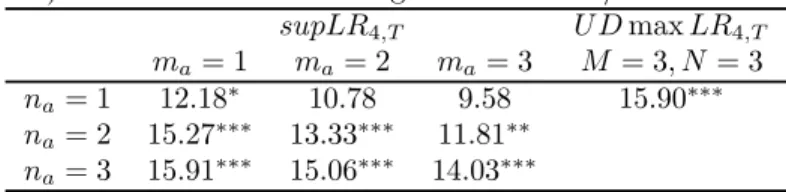
For TP-5 to TP-7, the critical values of the limit distributions are available in Bai and Perron (1998, 2003b) for N or M equal to 5. For TP-5 and TP-6, the results are valid for martingale di¤erences or serially correlated errors. This is not the case for TP-7 and TP-8 for reasons discussed above. We then consider the maximum of the Wald-type tests discussed Section 4.2. The limit distribution applicable to TP-8 is new. Table 1 presents critical values obtained using simulations as discussed above for the case of a …xed number of breaks under H1, for" = 0:1; 0:15, and 0:20, and values of M and N up to 2; see Perron and Yamamoto (2019b) for additional critical values with M; N = 2;3;4:
4.4 Testing for an additional break
We now consider TP-9 and TP-10, which assess whether including an additional break is warranted. Let(Te1c; :::;Temc;Te1v; :::;Tenv)be the estimates of the break dates in and 2 obtained jointly by maximizing the quasi-likelihood function assumingm breaks in andn breaks in
2. For TP-9, the issue is whether an additional break in is present. The test is supSeq9;T (m+ 1; njm; n) = max
1 j m+1 sup2 c j;" log ^LT(Te1c; :::;Te c j 1; ;Te c j; :::;Te c m;Te v 1; :::;Te v n) log ^LT(Te1c; :::;Te c m;Te v 1; :::;Te v n) where c
j;" =f ;Tejc 1+ (Tejc Tejc 1)" Tejc (Tejc Tejc 1)"g. This amounts to performing m+ 1 tests for a single break in for each of the m + 1 regimes de…ned by the partition fTe1c; :::;Temcg. Note that there are di¤erent scenarios when allowing breaks in and in 2 to happen at di¤erent dates, since(Te1c; :::;Temc)and (Te1v; :::;Tenv)can partly or completely overlap or be altogether di¤erent. This implies two possible cases: 1) if the n break dates in 2 are a subset of the m break dates in , there is no variance break between Tec
j 1 and Tejc; 2) otherwise, there is one or more variance breaks betweenTec
j 1 andTejc. In either cases, one can appeal to the results of Theorem 1(c) withma = 1since any value ofnais allowed, including 0. It is then easy to deduce that, in the case of martingale errors, the limit distribution of the test is, under Assumptions A2 and A3, limT!1P (supSeq9;T (m+ 1; njm; n) x) = Gq;"(x)
m+1
, where Gq;"(x) is the cumulative distribution function of the random variable sup 2 1;"jj(Wq( ) Wq(1))
2
jj=( (1 )), where 1;" =f ;" < <1 "g. The critical values of the distribution functionGq;"(x)
m+1
can be found in Bai and Perron (1998, 2003b). With serial correlation in the errors, the principle is the same except that the statistic is based on the robust Wald testsupF3;T as de…ned by (13) applied for a one break test to each segment. For TP-10, similar considerations apply. Here the issue is whether an additional break in the variance is present. The test statistic is
supSeq10;T(m; n+ 1jm; n) = (2=^) max
1 i n+1 sup2 v i;" log ^LT(Te1c; :::;Te c m;Te v 1; :::;Te v i 1; ;Te v i ; :::;Te v m) log ^LT(Te1c; :::;Temc;Te1v; :::;Tenv)
where vi;"=f ;Teiv 1+ (Teiv Teiv 1)" Teiv (Teiv Teiv 1)"g. The correction factor (2=^) is needed to ensure that the limit distribution of the test is free of nuisance parameters when the errors are allowed to be non-normal, serially correlated and conditionally heteroskedastic. One can then use part (b) of Theorem 1 to deduce that, under A1 and A3 applied to each segments under H0: limT!1P(supSeq10;T(m; n+ 1jm; n) x) =G1;"(x)n+1.
4.5 Local asymptotic power
Supplement D contains details about the local asymptotic power function of selected tests. We brie‡y summarize the relevant results. We consider model (1) focusing on the case of n=m= 1 with the following assumptions.
Assumption L1: Assumptions A1 and A3 hold with 20 10 = = p
T. We also have T 1=2P[T s]
t=1[(ut)2 1] ) W(s) with = limT!1var(T 1=2PTt=1[(ut)2 1]) and T 1P[T s]
t=1(ut)2 p
!s uniformly ins.
Assumption L2: Assumptions A2 and A3 hold with 02 01 = =pT :
We derive the local asymptotic power of the testssupLR2;T(n = 1; m= 1; "jn= 0; m= 1) and supLR3;T(m = 1; n = 1; "jm = 0; n = 1) and the corresponding tests with no nuisance breaks accounted for, i.e.,supLR1;T and the standard supLRT test. Lemma S.1 shows that the local asymptotic power of the supLR2;T test coincides with that of supLR1;T except that the set of permissible break dates cv; is smaller than v; , which has no practical e¤ect. Lemma S.2 shows that the local asymptotic power of the supLR3;T is the same as that of supLRT derived in Andrews (1993, Theorem 4), again except that the set of permissible break dates is v
c; instead of c; . Hence, when testing for changes in variance (resp., coe¢ cients) allowing for changes in coe¢ cients (resp., variance), we have the same local asymptotic poser function as when testing for changes in variance (resp., coe¢ cients) when no change in coe¢ cient (resp., variance) is present. Hence, there is no loss in local asymptotic power adopting our more general approach.
We also derived the local asymptotic power function of the CU SQ test (see (14) below for its de…nition) and compared it to that of the supLR1;T and supLR2;T tests. Figure S.1 shows the asymptotic local power functions of thesupLR1;T and CU SQ tests when a break in variance occurs at v0 = 0:3; 0:5 and 0:7 and no break occurs in the coe¢ cients. They show the local asymptotic power functions to be almost identical. Figure S.2 presents the local asymptotic power functions of the supLR2;T test when it accounts for a coe¢ cient break at c0 = 0:3; 0:5 or 0:7. It also shows, the local asymptotic power functions of the CU SQ test under the assumption of no break in the coe¢ cients. This simulation design gives an advantage to the CU SQ. Indeed, the power of the supLR2;T test is slightly lower when the variance and the coe¢ cient break dates coincide. This is because the permissible break dates around the true break date are not considered due to the concurrent nuisance break. However, the power loss of thesupLR2;T test is very minor. The power of both tests are almost identical even though the supLR2;T test considers a single nuisance break when the two breaks are far apart. i.e., the case of ( v0; c0) = (0:3;0:7)and (0:7;0:3).
5 Monte Carlo experiments
We now provide the results of simulation evidence to assess the size and power properties of some of the tests proposed; Section 5.1 for variance breaks, 5.2 for conditional tests, 5.3 for thesupLR4;T andU Dmaxtests. Supplement E provides additional results for thesupLR1;T and supLR2;T tests when the errors are non-normally distributed. Following Bai and Ng (2005), we use the following speci…cations: (a) thet distribution with 5 degrees of freedom, (b) a mixture of two normal distributions: v1I(z 0:5) +v2I(z > 0:5), where z U[0;1], v1 N( 1;1) and v2 N(1;1) (c) the 2 distribution with 5 degrees of freedom and (d) an exponential distribution ln(v),v U[0;1]. The results show that the exact size of the tests is similarly close to the nominal size. As expected, power is lower for all distributions, though the extent of the power loss is minor and the tests remain informative. Of interest is that our tests for changes in variance ratain their power advantage over the CU SQ test.
5.1 Testing for variance breaks only
We now consider the case of testing only for variance breaks assuming no change in . We investigate the properties of the following tests: thesupLR1;T (na; "jm=n= 0), abbreviated supLR1;T (na; ")and theU DmaxLR1;T for an unknown number of breaks up toN = 5. We also consider a corrected version of the CUSUM of squares test of Brown, Durbin and Evans (1975), as extended by Deng and Perron (2008), given by
CU SQ= sup 2[0;1]jT 1=2[P[tT=1]evt2 ([T ]=T)PTt=1evt2]j='^1a=2 (14) with '^a=T 1P(T 1) j= (T 1)!(j; bT) PT t=jjj+1^t^t j, where ^t=ev2t ^, ^ 2 =T 1PT t=1ev 2 t and e
vt denotes the recursive residuals. Also !(j; bT) is the Quadratic Spectral kernel and the bandwidthbT is selected using Andrews’(1991) method with an AR(1) approximation. The aim of the design is to address the following issues: a) the size of the supLR1;T (na; ") and U DmaxLR1;T tests; b) the relative power of the three tests; c) the power losses obtained when under-specifying the number of breaks; d) the relative power of the U DmaxLR1;T compared tosupLR1;T(na; ")withnaspeci…ed to be the true number of breaks. We consider a dynamic model with GARCH errors, for which the DGP is given by yt = c+ yt 1 +et, et = utpht; ut i:i:d: N(0;1), ht = 1 + 21 (t >[:5T]) + e2t 1 + ht 1, where we set h0 = 1=(1 ), c = 0:5, 1 = 0:1, and " = 0:15. We consider = 0:2, 0:7 and the GARCH(1,1) coe¢ cients are set to = 0:1, 0:3, 0:5and = 0:2: The size and power of 5% nominal size tests are evaluated at T = 100; 200. The magnitude of the change 2 varies
between 0 (size) and 0:3. The results are presented in Table 2. The supLR1;T (1; ") and U DmaxLR1;T tests show size distortions when = 0:5 with T = 100 but the size is close to 5% when T = 200. The CU SQ test is slightly undersized. The U DmaxLR1;T test has power close to that of supLR1;T (1; "), despite having a broader range of alternatives. The power of the latter two tests dominates that ofCU SQespecially whenT = 100. Supplement F shows the results to be robust for a static mean model with normal errors.
We now turn to a case with two breaks in variance. The DGP is yt = et; et i:i:d: N(0;1 + 1(T1v < t T2v)), i.e., the variance increases at T1v and returns to its original level at Tv
2. We consider two scenarios: fT1v = [:3T], T2v = [:6T]g and fT1v = [:2T], T2v = [:8T]g. We set T = 200 and " = 0:10, 0:15. The magnitude of the break in 2 varies between = 0 (size) and = 3. We again consider the U DmaxLR1;T test with N = 5 but include both thesupLR1;T(1; ")test for a single break and thesupLR1;T (2; ")test for two breaks to assess the extent of power gains when specifying the correct number of breaks. The results are presented in Table 3. Consider …rst the size of the tests. ThesupLR1;T (1; "),supLR1;T(2; ") and U DmaxLR1;T are slightly conservative and theCU SQ even more so with an exact size of 0.025. As expected, power increases as " increases since the range of alternatives is smaller. When comparing the supLR1;T (1; ") and supLR1;T(2; ") tests, the latter is more powerful, indicating that allowing for the correct number of breaks improves power. The U DmaxLR1;T has power between those of the supLR1;T (1; ") and supLR1;T (2; ") tests. These tests are considerably more powerful than the CU SQ, which has little power.
5.2 Conditional tests
We now consider the properties of the tests that condition on either breaks in coe¢ cients (resp., variance) when testing for changes in variance (resp., coe¢ cients). Consider …rst the size and power ofsupLR2;T (ma; na; "jn = 0; ma)which tests fornachanges in 2 conditional on ma changes in with " = 0:1;0:2. We set ma =na = 1 and the DGP is a simple mean shift model with a change of magnitude 2 at mid-sample with i:i:d: normal errors having a change in variance of magnitude (under H1) that occurs at [0:25T]. The results for size are presented in Table 4. The test is slightly conservative and more so as the trimming is larger. This is due to the fact that the limit distribution used is an upper bound. The results for power are presented in Table 5. It increases rapidly with the magnitude of the variance break and with T. It also marginally increases with the value of the trimming".
We next investigate the size and power of supLR3;T(ma; na; "jm = 0; na) which tests for ma changes in conditional on na changes in 2 with " = 0:1;0:2. We again set ma =
na = 1 and consider the mean model in which 2 changes at mid-sample. We also consider an AR(1) model yt = c+ yt 1 +et with c = 0:5; = 0:5 and et being i:i:d: normal errors having a change in variance at [0:5T] with magnitude . This is done to investigate potential size distortions due to large variance changes. As discussed in Section 4.1, a change in variance induces a change in the marginal distribution of the regressors when lagged dependent variables are included. The results for the size of the tests are presented in Table 6. The size under the mean model is close to the nominal level but the test becomes conservative as"increases since the limiting distribution used is a bound. The size under the AR(1) model is very similar with the distortions being even smaller. This indicates that the shrinking variance assumption is not binding. The results for power are presented in Table 7 for the mean model with a coe¢ cient change at [0:25T]. The power quickly increases as the break magnitude and T increase. The power again marginally increases with ".
5.3 Size and power of the supLR4;T and U DmaxLR4;T tests
We now present results about the properties of the supLR4;T and U DmaxLR4;T (simply labelled U Dmax) tests. To this end, we use a model with GARCH(1,1) errors so that the DGP is yt = et with et = ut
p
ht; where ut i:i:d: N(0;1), ht = 1 + e2t 1 + ht 1, h0 = 1=(1 ), 1 = 1, = 0:2 and takes values 0:1, 0:3, 0:5. Also, " = 0:1, 0:2. For the U Dmax test, M = N = 2 and for the supLR4;T test, we consider the following combinations: a) ma =na= 1, b)ma= 1,na= 2, c) ma= 2,na= 1. We set T = 100, 200. The results are presented in Table 8 and they show that the size is close to or slightly lower than the nominal 5% level (some cases have slight liberal size distortions when T = 100, which, however, decrease when T = 200). Supplement G shows that the tests have good sizes when the errors are i.i.d. normal.
We now consider the power of these tests. Since some partial results for the one break case are available in Tables S.6-S.7 for the supLR4;T test, we concentrate on the case with a di¤erent number of breaks in coe¢ cients and in variance. We also only consider i.i.d. normal errors though the hybrid-type correction is still applied. Table 9 presents the results for the case with one break in coe¢ cient and two breaks in variance, in which case the DGP is yt = 1 + 21(t > Tc) +et, et i:i:d: N(0;1 + 1(T1v < t T2v)) with 1 = 0, 2 = and " = 0:1. Five di¤erent con…gurations of break dates are considered. We analyze two forms of thesupLR4;T test: a) one testing for a single break in both mean and variance, b) one correctly testing for two changes in variance and one change in mean. This is done to investigate the extent of the power di¤erences when underspecifying the number of breaks.
As expected, the power increases rapidly with and withT. With the DGP used, the power is similar whether accounting for one or (correctly) two breaks in variance and the power of the U Dmax test is also similar to the power of both versions of the supLR4;T test. This may, however, be DGP speci…c. Table 10 presents the results for the case with two breaks in coe¢ cient and one break in variance, with the DGP given byyt= 1+ 21(T1c < t T2c)+et, et i:i:d: N(0;1 + 1(t > Tv)) with 1 = 0 and 2 = . Again, we consider two forms of the supLR4;T test: one testing for a single break in both mean and variance, one correctly testing for two changes in mean and one change in variance. Table 10 shows that for given values of and T, the power is lower than with one break in coe¢ cient and two breaks in variance. Also, theU Dmaxtest now has power between that of the test correctly specifying the type and number of breaks and that underspecifying the number of changes in mean. The di¤erence can be substantial and, as in Bai and Perron (2006), the power of theU Dmax test is close to that attainable when the type and number of breaks is correctly speci…ed
6 Estimating the numbers of breaks in coe¢ cients and in variance
To select the number of breaks in either the regression coe¢ cients or the error variance, the method suggested is a speci…c to general procedure that uses the sequential tests proposed in Section 4.4. We determine the number of coe¢ cients and variance breaks allowing for a given number of breaks in the other component. When selecting the number of breaks in , we consider TP-9 and the test supSeq9;T(m+ 1; Njm; N) is applied, starting with H0 :m = 0 and H1 : m = 1, where N is some pre-speci…ed maximum number of breaks in variance. Upon a rejection, we proceed toH0 :m= 1 versusH1 :m= 2, and so on until the test stops rejecting. Since the number of breaksnin 2 is unknown, contamination of the test statistics by unaccounted breaks in 2 must be avoided. This can be achieved imposing a maximum number N throughout. Similarly, to select the number of breaks in 2, TP-10 is considered and the test supSeq10;T(M; n+ 1jM; n)is used for n= 0;1; :::, until a non-rejection occurs. Again, some maximum number of breaks in the coe¢ cients M is imposed. To assess the …nite sample properties of these procedures, we performed a simple simulation experiment. Again, we setT = 200 and "= 0:15 and the basic DGP is:
yt = 1+ 21(t > Tc) +et; et i:i:d: N(0;1 + 1(t > Tv));
with 1 = 0 so that at most one break in either mean or variance occurs. We consider the following scenarios: a) no change in mean or variance, b) a change in mean only occurring at mid-sample, c) a change in variance only occurring at mid-sample, d) a change in both
mean and variance occurring at a common date (mid-sample); e) a change in both mean and variance occurring at di¤erent but close dates (Tc = [0:5T]; Tv = [0:7T]) or f) at di¤erent and distant dates (Tc = [0:25T]; Tv = [0:75T]). Di¤erent magnitudes of breaks are considered. The procedure is applied setting the maximum number of breaks toM = 2 and N = 2 (i.e., four breaks overall). We also considered a split-sample method discussed in Supplement H. The results are presented in Tables 11 and S.4. The procedures work quite well in selecting the correct number and type of breaks. There are cases, however, where the probability of correct selection is quite low with the split-sample method, e.g., when both changes in mean and variance are not large and occur at di¤erent dates, especially far apart. The speci…c to general approach tests for breaks in coe¢ cients and variance separately allowing the other component to have unknown breaks, which can avoid segmentations and lead to power gains. The probabilities of selecting the correct number of each type of breaks are high with this approach (higher than with the split-sample method, see Table S.10) when the changes are not large and the break dates are di¤erent. Hence, we recommend this procedure in practice.
7 Empirical examples
We investigate structural changes in the conditional mean and in the error variance of US in‡ation, quarterly from 1959:1 to 2018:4. For comparison purposes, we use Stock and Wat-son’s (2002) transformation to achieve stationarity, i.e., we transform the GDP de‡ator (Xt) into annual changes of the quarterly in‡ation rate asYt= 100[ln(Xt=Xt 1) ln(Xt 4=Xt 5)]. The resulting series is presented in Figure 1. We use a simple AR(4) model of the form Yt = +P4j=1 jYt j+et. Using the sample from 1959:1 to 2002:3 and a two-step procedure, Stock and Watson (2002) found strong evidence of a structural change in the conditional mean but no or weak evidence of changes in the error variance. Table 12(a) reports the supLR4;T and the U Dmax4;T tests. They suggest at least one change in either or both the coe¢ cients and the variance. Table 12(b) presents the results when testing for changes in the coe¢ cients, allowing for changes in the variance. Consistent with Stock and Watson (2002), we obtain strong evidence of a change in the conditional mean coe¢ cients if we as-sume no change in the error variance (supLR3;T with ma = 1 and U Dmax3;T tests, both with na = 0). The sequential procedure using thesupSeq10;T test con…rms that a one break speci…cation is preferred with the break date estimated at 1973:2, as in Stock and Watson (2002). However, any evidence of changes in the conditional mean disappears once we jointly consider structural changes in the error variance. To assess whether changes in variance are indeed present when accounting for potential changes in the regression coe¢ cients, Table
12(c) presents the results of thesupLR2;T and theU Dmax2;T tests. These suggest the pres-ence of breaks in the variance. The sequential testsupSeq9;T suggests 3 breaks estimated at 1971:2, 1983:2 and 2006:3 when ma = 0. Hence, contrary to Stock and Watson (2002), we conclude for three structural changes in the error variance and no change in the conditional mean. The changes are such that the variance went from 1.00 to 3.29 in 1971:2, then to 0.49 in 1983:1 and to 1.42 in 2006:3.
We now consider the US ex-post real interest rate and use the same quarterly series from 1961:1-1986:3 (see Figure 2), as in Garcia and Perron (1996) and Bai and Perron (2003a) since it is a widely used example involving important mean shifts, though variance shifts have not been investigated. We use a model with only a constant as regressor (i.e.,zt=f1g) and account for serial correlations in the errors term via a HAC variance estimator using the hybrid method. The estimate of the scaling factor , see (8), also uses the hybrid method. Bai and Perron (2003a) found two large mean shifts in 1972:3 and 1980:3 and a small change in 1966:4 using the sequential procedure proposed in Bai and Perron (1998, 2003a), which allows for variance breaks occurring at the same time as the mean breaks, though not at di¤erent times. Here, the focus is on assessing whether changes in variances are present and if so whether and how the changes in mean present a¤ect the results. Because they found three breaks in the mean, we use our tests with ma up to 3 and na up to 2. The trimming parameter " = 0:15 is used. The critical values of both tests when M = 3 are provided in Perron and Yamamoto (2019b). Table 13(a) presents the results for the supLR4;T and the U DmaxLR4;T tests, which suggest clear rejections of the null hypothesis of no breaks. Table 13(b) presents the results when testing for mean breaks accounting for possible variance breaks using the supLR3;T and the U DmaxLR3;T tests and also the supSeq10;T test to determine the number of breaks. We obtain evidence for two mean breaks in 1972:3 and 1980:3, irrespective of how many variance breaks are accounted for. However, we do not …nd evidence for a mean break in 1966:4. To investigate the presence of variance changes, Table 13(c) presents the results of the tests for variance breaks accounting for mean breaks. If we account for no mean breaks (ma = 0), two variance breaks are found in 1972:3 and 1981:2; the former is the same and the latter is close to the dates of the two large mean breaks. However, if one mean break is allowed (ma= 1), only one variance break is found in 1972:3, which suggests that the variance break in 1981:2 was a false rejection due to the ignored mean break. The next issue is whether the 1972:3 variance break is spurious. To see this, we account for two breaks in the mean (ma = 2) and …nd again two breaks in the variance; one in 1972:3 and the other is in 1964:3. The variance break in 1964:3 is relatively small and
was thereby masked when the two mean breaks were not accounted for. More importantly, we again obtain no evidence for a break around 1980:3 but rather one in 1972:3. In addition, if we account for three (ma = 3) mean breaks, we also …nd a variance break in 1972:3. Therefore, we conclude that both the mean and the variance changed in 1972:3 but only the mean changed in 1980:3, while only the variance changed in 1964:3. This latter change may be responsible for Bai and Perron’s (2003a) …nding of an additional mean break in 1966:4 using tests that allow for variance changes, though at the same dates as the mean changes. The change are such that the mean went from 1.36 to -1.80 in 1972:3 and to 5.64 in 1980:3, while the variance changed from 1.09 to 1.87 in 1964:3 and then to 6.91 in 1972:3.
8 Conclusion
This paper provided tools for testing for multiple structural breaks in the error variance in the linear regression model with or without the presence of breaks in the regression coe¢ cients. An innovation is that we do not impose any restrictions on the break dates, i.e., the breaks in the regression coe¢ cients and in the variance can happen at the same time or at di¤erent times. We proposed statistics with asymptotic distributions invariant to nuisance parameters and valid with non-normal errors and conditional heteroskedasticity, as well as serial correlation. Extensive simulations of the …nite sample properties show that our procedures perform well in terms of size and power. A speci…c to general procedure to estimate the number and type of breaks based on a proposed sequential test is shown to perform well in selecting the number and types of breaks.
Appendix
Proof of Theorem 1: Part (a) follows from Qu and Perron (2007a, Theorem 5) under A1. For part (b), supLR2;T(ma; na; "jn= 0; ma) = 2[log ^LT(Te1c; :::;Te c ma;Te v 1; :::;Te v na) logLeT( ^T c 1; :::;T^ c ma)] = Tloge2 Pna+1 i=1 (Te v i Te v i 1) log ^ 2 i = Pna i=1[Te v i+1loge 2 1;i+1 Teivloge 2 1;i (Teiv+1 Teiv) log ^ 2 i+1] +Te1v(loge 2 1;1 log ^ 2 1) wheree21;i= (Tev i ) 1 PTev i
t=1(yt x0te zt0et;j)2 withet;j =ej forT^jc 1 < t T^jc (also let 0 t;j = 0 j for Tc0 j 1 < t Tjc0) (j = 1; :::; ma+ 1) and ^2i = (Teiv Teiv 1) 1 PTev i t=Tev i 1+1 (yt x0t^ zt0^t;j)2. Applying a Taylor expansion to loge21;i+1, loge21;i and log ^2i+1 aroundlog 2
0, we obtain supLR2;T (ma; na; "jn = 0; ma) = Pna i=1(F i 1;T +F i 2;T) +op(1) where F1i;T = ( 20) 1[Teiv+1e21;i+1 Teive21;i (Teiv+1 Teiv)^2i+1] = ( 20) 1PTe v i+1 t=Tev i+1 h (yt x0te zt0et;j)2 (yt x0t^ z0t^t;j)2 i and F2i;T = (1=2)[Teiv+1(e 2 1;i+1 20 2 0 )2 Teiv(e 2 1;i 20 2 0 )2 (Teiv+1 Teiv)(^ 2 i+1 20 2 0 )2] = (1=2)(I+II+III): (A.1)
We …rst show that F1i;T =op(1). We can expressF1i;T as
( 20) 1 2 6 6 6 6 6 6 4 (Ui+1+Xi+1( 0 e) +Zi+1( 0t;j et;j))0(Ui+1+Xi+1( 0 e) +Zi+1( 0t;j et;j)) (Ui+1+Xi+1( 0 ^) +Zi+1( 0t;j ^t;j))0(Ui+1+Xi+1( 0 ^) +Zi+1( 0t;j ^t;j)) 3 7 7 7 7 7 7 5 = ( 20) 1 2 6 6 6 6 6 6 4 (^ e)0X0 i+1Xi+1(^ e) + (^t;j et;j)0Zi0+1Zi+1(^t;j et;j) +(^ e)0Xi0+1Zi+1(^t;j et;j) + 2( ^)0Xi0+1Xi+1(^ e) +2( t;j0 ^t;j)0Zi0+1Zi+1(^t;j et;j) + 2(^ e)0Xi0+1Zi+1( 0t;j ^t;j) +2( ^)0Xi0+1Zi+1(^t;j et;j) + 2(^ e)0Xi0+1Ui+1+ 2(^t;j et;j)0Zi0+1Ui+1 3 7 7 7 7 7 7 5 :
The result follows using the facts that X0
i+1Xi+1 = Op(T), Zi0+1Zi+1 = Op(T), Xi0+1Zi+1 = Op(T), Xi0+1Ui+1 = Op(T1=2) and Zi0+1Ui+1 = Op(T1=2). Also, since under H0 with A1, the estimates of the break fractions converge to the true break fractions at a fast enough rate so that the estimates of the parameters of the models are consistent and have the same limit distribution as when the break dates are known, we have: 0 ^ = Op(T 1=2),
0
t;j ^t;j =Op(T 1=2), ^ e=op(T 1=2) and^t;j et;j =op(T 1=2). The last two quantities areop(T 1=2)since
p
T(^ 0)and pT(e 0)have the same limit distribution underH0, and likewise forpT(^t;j 0t;j) and
p T(et;j 0t;j). For F2i;T, p I = (Teiv+1) 1=2PTe v i+1 t=1 [f(yt x0te zt0et;j)= 0g2 1] = (Teiv+1) 1=2PTeiv+1 t=1 (ut= 0)2 1 +op(1) ) p W( vi+1)= q v i+1
by A1. Similarly, pII )p W( vi)=p vi and p III = [(Teiv+1 Teiv)=T] 1=2T 1=2PT v i+1 t=Tv i+1[(ut= 0) 2 1] +o p(1) = [(Teiv+1 Teiv)=T] 1=2fT 1=2PT v i+1 t=1 [(ut= 0)2 1] T 1=2 PTv i t=1[(ut= 0)2 1]g+op(1) ) p [W( vi+1) W( vi)]=q vi+1 vi: Therefore, F2i;T ) ( =2) W 2( v i+1) v i+1 W2( vi) v i (W( vi+1) W( vi))2 v i+1 v i = ( =2)( v iW( v i+1) v i+1W( v i))2 v i+1 v i( v i+1 v i) : This yields supLR2;T(ma; na; "jn= 0; ma) ) sup ( v1;:::; vna)2 cv;" na P i=1 2 ( viW( vi+1) vi+1W( vi))2 v i+1 v i( v i+1 v i) sup ( v1;:::; vna)2 v;" na P i=1 2 ( viW( vi+1) vi+1W( vi))2 v i+1 v i( v i+1 v i) because cv;" v;". For part (c),
supLR3;T (ma; na; "jm = 0; na) = 2[log ^LT(Te1c; :::;Te c ma;Te v 1; :::;Te v na) logLeT( ^T v 1; :::;T^ v na)] = Pna+1 i=1 ( ^T v i T^ v i 1) loge 2 i Pna+1 i=1 (Te v i Te v i 1) log ^ 2 i where e2i = ( ^Tiv T^iv1) 1 PT^v i t= ^Tv i 1+1 (yt x0te zt0e)2 and ^ 2 i = (Teiv Teiv 1) 1 PTev i t=Tev i 1+1 (yt x0
t^ zt0^t;j)2. Applying a Taylor expansion onloge2i and log ^ 2
i aroundlog 2i0, we obtain supLR3;T (ma; na; "jm = 0; na) =Pni=1a+1(F1i;T +F
i
where Fi 1;T = ( ^Tiv T^iv 1)(e 2 i= 2i0) (Teiv Teiv 1)(^ 2 i= 2i0)and F2i;T = (1=2)[( ^Tiv T^iv 1)([e2i 2i0]= 2i0)2 (Teiv Teiv 1)([^2i 2i0]= 2i0)2]: We …rst show that Fi 2;T =op(1) as follows. We have: F2i;T = (1=2)[( ^Tiv T^iv1)(e 2 i 2i0 2 i0 )2 (Teiv Teiv 1)(^ 2 i 2i0 2 i0 )2] = (1=2)[T 1( ^Tiv T^iv 1)[T1=2(e 2 i 2i0 2 i0 )]2 T 1(Teiv Teiv1)[T1=2(^ 2 i 2i0 2 i0 )]2] where [( ^Tiv T^iv1)=T][pT(e2i 2i0)= 2i0]2 and [(Teiv Teiv 1)=T][pT(^2i 2i0)= 2i0]2 have the same limit distribution under A3. ForFi
1;T, let 0 = 10 without loss of generality, then
Pna+1 i=1 F i 1;T = ( 2 0) 1Pna+1 i=1 h ( ^Tiv T^iv 1)e2i (Teiv Teiv 1)^2ii +( 20) 1Pna+1 i=1 ([ 2 i0 2 0]= 2 i0) h ( ^Tiv T^iv 1)e2i (Teiv Teiv 1)^2ii: The …rst term becomes,
( 20) 1Pna+1 i=1 h ( ^Tiv T^iv 1)e2i (Teiv Teiv1)^2ii = ( 20) 1PTt=1[(yt x0te z0te) 2 (y t x0t^ zt0^t;j)2] (A.2) = ( 20) 1Pma j=1 PTec j+1 t=1 (yt x0te zt0e) 2 PTejc t=1(yt x0te zt0e) 2 PTejc+1 t=Tec j+1 (yt x0t^ zt0^j+1)2 +( 20) 1PTe1c t=1(yt x0te zt0e) 2 ( 20) 1PTe1c t=1(yt x0t^ zt0^1)2 = ( 20) 1fPma j=1[D r(1; j+ 1) Dr(1; j) Du(j+ 1)] +Dr(1;1) Du(1) g; whereDr(1; j) = PTejc t=1(yt x0te zt0e)2 and Du(j) = PTec j t=Tec j 1+1 (yt x0t^ zt0^j)2. The second term is op(1) by A3. Using similar derivations as in Qu and Perron (2007b), we obtain
Dr(1; j+ 1) Dr(1; j) Du(j + 1) = U1:0j+1Z1:j+1(Z1:0j+1Z1:j+1) 1Z1:0j+1U1:j+1+U1:0jZ1:j(Z1:0 jZ1:j) 1Z1:0 jU1:j +Uj0+1Zj+1(Zj0+1Zj+1) 1Zj0+1Uj+1+op(1); ) c jWq( cj+1) c j+1Wq( cj) 2 c j+1 c j( c j+1 c j) by A2. This yields
supLR3;T(ma; na; "jm= 0; na) ) sup ( c 1;:::; cma)2 vc;" ma X j=1 c jWq( cj+1) c j+1Wq( cj) 2 c j+1 c j( c j+1 c j) ; sup ( c 1;:::; cma)2 c;" ma X j=1 c jWq( cj+1) c j+1Wq( cj) 2 c j+1 c j( c j+1 c j) ;