A Comparison of Wavelet and Simplicity-Based Heart Sound and Murmur Segmentation Methods

A COMPARISON OF WAVELET AND SIMPLICITY-BASED HEART SOUND AND MURMUR SEGMENTATION METHODS

A Thesis presented to

the Faculty of California Polytechnic State University, San Luis Obispo

In Partial Fulfillment

of the Requirements for the Degree Master of Science in Electrical Engineering

by

Joshua David Korven September 2016

ii © 2016

Joshua David Korven ALL RIGHTS RESERVED

iii

COMMITTEE MEMBERSHIP

TITLE: A Comparison of Wavelet and Simplicity-Based Heart Sound and Murmur Segmentation Methods

AUTHOR: Joshua David Korven

DATE SUBMITTED: September 2016

COMMITTEE CHAIR: Wayne Pilkington, Ph.D.

Associate Professor of Electrical Engineering

COMMITTEE MEMBER: Jane Zhang, Ph.D.

Professor of Electrical Engineering

COMMITTEE MEMBER: John A. Saghri, Ph.D.

iv ABSTRACT

A Comparison of Wavelet and Simplicity-Based Heart Sound and Murmur Segmentation Methods

Joshua David Korven

Stethoscopes are the most commonly used medical devices for diagnosing heart conditions because they are inexpensive, noninvasive, and light enough to be carried around by a clinician. Auscultation with a stethoscope requires considerable skill and experience, but the introduction of digital stethoscopes allows for the automation of this task. Auscultation waveform segmentation, which is the process of determining the boundaries of heart sound and murmur segments, is the primary challenge in automating the diagnosis of various heart conditions. The purpose of this thesis is to improve the accuracy and efficiency of established techniques for detecting, segmenting, and classifying heart sounds and murmurs in digitized phonocardiogram audio files. Two separate segmentation techniques based on the discrete wavelet transform (DWT) and the simplicity transform are integrated into a MATLAB software system that is capable of automatically detecting and classifying sound segments.

The performance of the two segmentation methods for recognizing normal heart sounds and several different heart murmurs is compared by quantifying the results with clinical and technical metrics. The two clinical metrics are the false negative detection rate (FNDR) and the false positive detection rate (FPDR), which count heart cycles rather than sound segments. The wavelet and simplicity methods have a 4% and 9% respective FNDR, so it is unlikely that either method would not detect a heart condition. However, the 22% and 0% respective FPDR signifies that the wavelet method is likely to detect false heart conditions, while the simplicity method is not. The two technical metrics are the true

v

murmur detection rate (TMDR) and the false murmur detection rate (FMDR), which count sound segments rather than heart cycles. Both methods are equally likely to detect true murmurs given their 83% TMDR. However, the 13% and 0% respective FMDR implies that the wavelet method is susceptible to detecting false murmurs, while the simplicity method is not. Simplicity-based segmentation, therefore, demonstrates superior performance to wavelet-based segmentation, as both are equally likely to detect true murmurs, but only the simplicity method has no chance of detecting false murmurs.

Keywords: Phonocardiogram, PCG, Stethoscope, Segmentation, Discrete Wavelet Transform, DWT, Simplicity Transform, Beamforming

vi

TABLE OF CONTENTS

Page

LIST OF TABLES ... xii

LIST OF FIGURES ... xiv

CHAPTER 1 INTRODUCTION ... 1

1.1 Cardiac Structure and Function ... 1

1.2 Cardiac Cycle ... 3

1.3 Auscultation, Heart Sounds, & Murmurs ... 4

1.4 Heart Sound and Murmur Segmentation Goals ... 9

1.5 Literature Review ... 10

1.6 Proposed Modifications to the Established Methods ... 12

2 VIABILITY OF USING A STETHOSCOPE ARRAY FOR IMPROVED HEART SOUND DETECTION ... 14

2.1 Introduction ... 14

2.2 Multiple Input Stethoscope ... 14

2.3 Beamforming ... 15 2.4 Acoustic Aperture... 16 2.5 Directivity Pattern ... 18 2.6 Aperture Array ... 19 2.7 Beamforming ... 20 2.8 Simulation Results ... 22 2.9 Discussion ... 30

3 SEGMENTATION ALGORITHMS AND CONCEPTS ... 31

vii

3.2 Wavelet Transform ... 35

3.2.1 Continuous Wavelet Transform ... 35

3.2.2 Discrete Wavelet Transform ... 36

3.3 Simplicity Transform ... 37

3.3.1 Complexity and Simplicity ... 37

3.3.2 Dynamical Systems ... 39

3.3.3 The Method of Delays ... 40

3.3.4 Eigenvalue Decomposition and the Singular Spectrum ... 43

3.3.5 Shannon Entropy ... 44

3.4 Piecewise Constant Denoising ... 47

3.5 Potts Functional ... 53

4 SEGMENTATION SYSTEM IMPLEMENTATION ... 56

4.1 System Overview ... 56

4.1.1 Introduction ... 56

4.1.2 Properties and Methods ... 56

4.1.3 PCG Retrieval ... 61

4.1.4 Wavelet filtering ... 62

4.1.5 Segmentation ... 65

4.1.6 Storing and summarizing results ... 67

4.1.7 Displaying results ... 69

4.2 Wavelet-based Segmentation ... 71

4.2.1 Heart Sound Segmentation ... 71

4.2.2 Removing Murmurs from Heart Sound Segments ... 76

4.2.3 Separating Split Heart Sounds ... 79

4.2.4 Heart Cycle Segmentation ... 81

viii

4.2.6 Heart Sound and Murmur Classification ... 84

4.3 Simplicity-based Segmentation ... 87

4.3.1 Simplicity Waveform Filtering ... 87

4.3.2 Piecewise Constant Approximation ... 88

4.3.3 Heart Sound and Murmur Segmentation ... 91

4.3.4 Split Sound Detection, Heart Cycle Segmentation, and Sound Segment Classification ... 92

5 SEGMENTATION RESULTS ... 94

5.1 Introduction ... 94

5.1.1 Sound File Datasets ... 94

5.1.2 Segmentation Errors and Detection Rates ... 94

5.1.3 False Negative and False Positive Detection Rates ... 96

5.2 Wavelet-Based Segmentation ... 99 5.2.1 Wavelet Constants ... 99 5.2.2 Wavelet Errors ... 100 5.2.3 Wavelet Results ... 114 5.3 Simplicity-Based Segmentation ... 117 5.3.1 Simplicity Constants... 117 5.3.2 Simplicity Errors ... 117

5.3.3 Simplicity Error Tables ... 126

5.4 Comparison of Segmentation Error Performance for the Two Methods ... 129

6 CONCLUSIONS AND FUTURE WORK ... 133

REFERENCES ... 135

APPENDICES A. Scripts ... 140

ix A.1.1 chp4_seg.m ... 140 A.1.2 energy_functions.m ... 140 A.1.3 heart_sounds.m ... 141 A.1.4 PCG_FFT.m ... 142 A.1.5 PCG_simpl.m ... 143 A.1.6 rect_sinc.m ... 143 A.1.7 singular_spectra.m ... 144 A.2 Results ... 145 A.2.1 batch.m ... 145 A.2.2 beamforming.m ... 146 A.2.3 dwt_michigan.m ... 147 A.2.4 dwt_littmann.m ... 147 A.2.5 simpl_michigan.m ... 148 A.2.6 simpl_littmann.m ... 149 B. Functions ... 151 B.1 Beamforming ... 151 B.1.1 beam_pattern.m ... 151 B.1.2 beamform.m ... 152 B.1.3 dist_mat.m ... 153 B.1.4 isAliased.m ... 153 B.2 DWT ... 154 B.2.1 coef_plot.m ... 154 B.2.2 coef_rng.m ... 155 B.3 Main ... 155 B.3.1 batch_segment.m ... 155 B.3.2 find_heart_cycles.m ... 156

x B.3.3 katz_fd.m ... 158 B.3.4 lbl_sounds.m ... 159 B.3.5 levels2seg.m ... 162 B.3.6 limit_HS.m ... 163 B.3.7 load_PCG.m ... 164 B.3.8 peak_peel.m ... 166 B.3.9 split_HS.m ... 167 B.3.10 st.m ... 169 B.4 Miscellaneous ... 170 B.4.1 closest.m ... 170 B.4.2 energy.m ... 171 B.4.3 env.m ... 171 B.4.4 nfft.m ... 171 B.4.5 normalize.m ... 172 B.4.6 pcg_descr.m ... 172 B.4.7 rect.m ... 172 B.4.8 shannon_energy.m ... 172 B.4.9 smooth.m ... 173 B.4.10 time.m ... 174 B.5 Plotting ... 174 B.5.1 fmt_line_arg.m... 174 B.5.2 horiz_line.m ... 175 B.5.3 plot_style.m ... 175 B.5.4 vert_line.m ... 175

C. Class Definitions and Methods ... 176

xi C.1.1 combine.m ... 176 C.1.2 find.m ... 176 C.1.3 levels.m ... 177 C.1.4 mask.m ... 177 C.1.5 segment.m ... 177 C.1.6 signal.m... 178 C.1.7 split.m ... 179 C.2 @stethoscope ... 179 C.2.1 cmp_PCG.m ... 179 C.2.2 dwt_filt.m ... 180 C.2.3 dwt_segment.m ... 180 C.2.4 plot.m ... 185 C.2.5 print.m ... 187 C.2.6 simpl_segment.m ... 188 C.2.7 stethoscope.m ... 192 C.2.8 title.m ... 196

xii LIST OF TABLES

Table Page

Table 4-1: stethoscope.m constant properties (SetAccess = immutable). ... 60

Table 4-2: stethoscope.m constant properties (SetAccess = public). ... 60

Table 4-3: stethoscope.m data properties (SetAccess = private). ... 61

Table 4-4: Set of all possible keys for conditions. ... 68

Table 4-5: Example keys and values for sscope.conditions. ... 68

Table 4-6: Heart sound and murmur segment color codes for plot(sscope). ... 70

Table 5-1: False negatives (Michigan). ... 97

Table 5-2: False positives (Michigan). ... 97

Table 5-3: False negatives (Littmann). ... 98

Table 5-4: False positives (Littmann). ... 98

Table 5-5: False negative detection rates (FNDR). ... 99

Table 5-6: False positive detection rates (FPDR). ... 99

Table 5-7: FNDR and FPDR comparison for wavelet and simplicity-based segmentation. ... 99

Table 5-8: Wavelet constants. ... 100

Table 5-9: Wavelet-based segmentation error labels and descriptions. ... 114

Table 5-10: Wavelet-based segmentation results (Michigan). ... 115

Table 5-11: Wavelet-based segmentation results (Littmann). ... 116

Table 5-12: Wavelet-based segmentation true murmur detection rate (TMDR). ... 116

Table 5-13: Wavelet-based segmentation false murmur detection rate (FMDR). ... 116

Table 5-14: Simplicity-based segmentation constants. ... 117

Table 5-15: Simplicity-based segmentation error labels and descriptions. ... 126

xiii

Table 5-17: Simplicity-based segmentation results (Littmann). ... 128 Table 5-18: Simplicity true murmur detection rate (TMDR). ... 128 Table 5-19: Simplicity false murmur detection rate (FMDR). ... 128 Table 5-20: Wavelet and simplicity-based segmentation performance

comparison. ... 129 Table 5-21: Wavelet and simplicity-based segmentation error comparisons

(Michigan). ... 131 Table 5-22: Wavelet and simplicity-based segmentation error comparisons

xiv LIST OF FIGURES

Figure Page

Figure 1-1: Blood flow through the heart (oxygen-poor blood is blue, oxygen-rich

blood is red). Adapted from [2]... 1

Figure 1-2: The heart’s chambers, veins, arteries, and valves [2]. ... 2

Figure 1-3: Diastole and systole [4]. ... 4

Figure 1-4: Labeled stethoscope [5]. ... 5

Figure 1-5: Phonocardiogram of a healthy heart [heart_sounds.m]. ... 6

Figure 1-6: PCG with a split S2 [heart_sounds.m]. ... 7

Figure 1-7: PCG with an S3 [heart_sounds.m]. ... 8

Figure 1-8: PCG with an S4 [heart_sounds.m]. ... 9

Figure 2-1: Precordial landmarks: Aortic (A), Pulmonic (P), Erb’s point (E), Tricuspid (T), and Mitral (M) [6]. ... 14

Figure 2-2: Spherical coordinate system [23]. ... 18

Figure 2-3: Stethoscope positions in the apparatus [beamforming.m]. ... 22

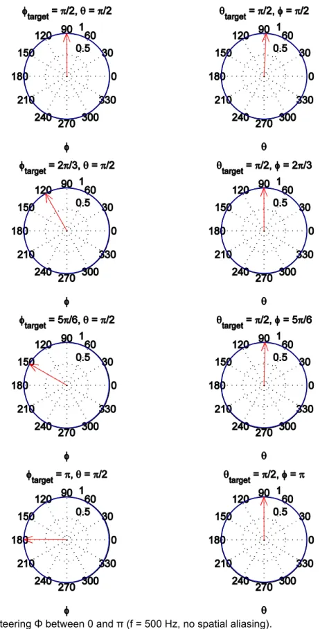
Figure 2-4: Steering Φ between 0 and π (f = 500 Hz, no spatial aliasing). ... 25

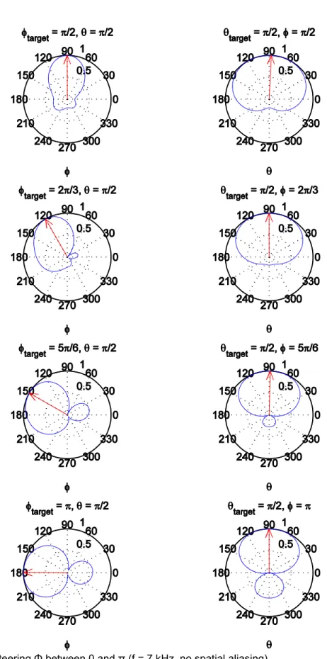
Figure 2-5: Steering Φ between 0 and π (f = 7 kHz, no spatial aliasing). ... 27

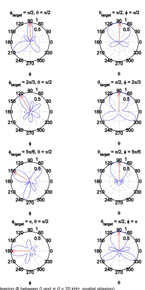
Figure 2-6: Steering Φ between 0 and π (f = 20 kHz, spatial aliasing). ... 29

Figure 3-1: PCG spectrum [PCG_FFT.m]. ... 34

Figure 3-2: Fourier transform of the sinc function [rect_sinc.m]. ... 38

Figure 3-3: Singular spectra comparison [singular_spectra.m]. ... 44

Figure 3-4: Raw simplicity waveform [PCG_simpl.m]. ... 48

Figure 3-5: Low pass filtering a rectangle causes ripple. The signal at the right was filtered with a higher order LPF than the signal at the left [31]. ... 49

xv

Figure 4-1: A range of approximation coefficients (left subplots) and detail coefficients (right subplots) are used to determine which approximation

coefficient is optimal for PCG reconstruction [chp4_seg.m]. ... 64 Figure 4-2: The original PCG (top subplot) has very little noise, so the filtered

PCG (bottom subplot) appears similar to the original PCG [chp4_seg.m]. ... 65 Figure 4-3: Graphical segmentation results for a PCG with systolic murmurs and

split S2 [chp4_seg.m]. ... 70 Figure 4-4: Shannon energy vs squared energy [energy_functions.m]. ... 72 Figure 4-5: Two peak peeling iterations. Subplot-1 separates the input signal into

the peak signal (blue) and the rejected signal (red). Subplot-2 displays the current output signal, which is a sum of the peaks from the current and previous

iterations [chp4_seg.m]. ... 74 Figure 4-6: PCG (subplot-1), wavelet reconstructed PCG (subplot-2), and peak

peeled Shannon energy with overlaid constant threshold (subplot-3)

[chp4_seg.m]. ... 76 Figure 4-7: Final heart cycle and heart sound segment boundaries overlaid on

the original PCG (subplot-1), troughs and thresholds for removing murmur samples from heart sound segments (subplot-2), murmur samples removed from heart sound segments (subplot-3), and segmented murmurs (subplot-4)

[chp4_seg.m]. ... 78 Figure 4-8: A heart sound segment containing split heart sounds is separated

into its component segments (subplot-3) [chp4_seg.m]. ... 80 Figure 4-9: The heart cycle boundary locations are approximated from spikes in

the autocorrelation of the PCG’s envelope (subplot-1). Afterwards, the cycle boundaries are shifted right and aligned with the nearest heart sound segment

xvi

Figure 4-10: The peak peeled fractal dimension extracts the sound peaks from the background noise (subplot-2), which are used to zero the non-sound

segments in the raw simplicity waveform (subplot-4) [chp4_seg.m]. ... 90 Figure 4-11: Threshold the normal heart sounds, extra heart sounds, and murmur segments by their simplicity levels (subplot-2) [chp4_seg.m]. ... 92 Figure 5-1: The first S1 is mistaken for a murmur because its maximum energy is

less than the energy threshold (subplot-3) [dwt_michigan.m]. ... 102 Figure 5-2: The first S1 segment is misidentified as a murmur, but the second S1

segment is properly identified (subplot-4). As a result, the first heart cycle’s start

boundary is moved from S1 to the nearest S2 (subplot-1) [dwt_michigan.m]. ... 103 Figure 5-3: The first S4 is misidentified as a murmur because its maximum

energy is less than the energy threshold (subplot-3) [dwt_littmann.m]. ... 105 Figure 5-4: The first S4 is misidentified as a murmur, but the second S4 is

acceptably misidentified as a split sound component (subplot-4). The cycle boundary locations are correct because S1 and S2 are properly identified

(subplot-1) [dwt_littmann.m]. ... 106 Figure 5-5: The diastolic murmur is misidentified as a heart sound because its

maximum energy is greater than the threshold (subplot-3) [dwt_littmann.m]... 108 Figure 5-6: The S4 peaks are below the segment thresholds (subplot-2) and are

therefore misidentified as murmurs (subplot-4) [dwt_michigan.m]. ... 110 Figure 5-7: The opening snap murmur is misidentified as a split S2 component

because the murmur’s peak is above the threshold (subplot-2). Also, the right boundary of S1 is repositioned despite the lack of a systolic murmur, and the

remaining piece is misidentified as a murmur [dwt_michigan.m]. ... 112 Figure 5-8: The cycle durations are too short because a peak near zero lag is

xvii

Figure 5-9: The diastolic murmur is misidentified as a heart sound because its

simplicity levels are greater than the HS threshold (subplot-2) [simpl_littmann.m]. ... 119 Figure 5-10: No heart sounds are detected because all segment levels are less

than the HS threshold (subplot-5) [simpl_littmann.m]. ... 121 Figure 5-11: The low amplitude diastolic murmurs (not visible) are undetected

because they were zeroed while peak peeling the fractal dimension (subplot-2). The corresponding simplicity values are zeroed (subplot-4), so the murmurs are

not segmented (subplot-5) [simpl_michigan.m]. ... 123 Figure 5-12: The summation gallops are misidentified as split sound components

because their simplicity levels are less than the extra HS threshold (subplot-2). This causes systole and diastole, and therefore S1 and S2, to be switched

1 1 Introduction

1.1 Cardiac Structure and Function

The purpose of the heart is to circulate blood throughout the body and supply the vital organs with oxygen, route the blood flow through the lungs to enrich the blood with oxygen, and dispose of the CO2 waste collected from the body. The most basic functional breakdown of the heart is to separate it into a right and a left side. Right and left are relative to the observer’s own frame of reference, so the orientation is reversed when the heart is presented on a diagram. The right side receives CO2-laden, oxygen-poor blood from the body and sends it to the lungs for CO2 removal and oxygen enrichment. Conversely, the left side receives oxygen-rich blood from the lungs and sends it to the rest of the body for oxygen distribution and CO2 waste collection. This process is synchronous because the left and right sides send and receive blood in unison [1]. The flow of blood through both sides of the heart is illustrated in Figure 1-1.

Figure 1-1: Blood flow through the heart (oxygen-poor blood is blue, oxygen-rich blood is red). Adapted from [2].

2

The two sides of the heart are separated by a muscular wall called the septum. Each side of the heart is further subdivided into two chambers, of which there are two types: atria and ventricles. The atria are the upper chambers that collect blood, and the ventricles are the lower chambers that pump blood. The heart has four chambers in total because each side has an atrium and a ventricle [1].

Blood enters the heart through veins and exits through arteries. The right atrium collects CO2-laden waste blood from the body through the venae cavae, where blood from the upper body flows through the superior vena cava, and blood from the lower body flows through the inferior vena cava. The right ventricle then sends the waste blood to the lungs through the pulmonary artery. At the same time, the left atrium collects oxygen-rich blood from the lungs through the pulmonary vein and sends the oxygen-rich blood to the body through the aorta. The heart’s chambers, veins, and arteries are labeled in Figure 1-2.

3

The heart is able to pump blood because valves separate the chambers and enable pressure gradients to form. Valves are passive structures made of connective tissue rather than muscle and are shaped like leaflets. The leaflet structure allows pressure differences alone to open or close valves, and it ensures that blood flows in a single direction without backflow into a previous chamber. A valve with leaflets pointing into a chamber will snap shut when the chamber’s pressure exceeds the surrounding environment. Likewise, a valve with leaflets protruding from a chamber will open when the chamber’s pressure exceeds the surrounding environment.

The atria and ventricles are separated by the atrioventricular valves: the tricuspid valve separates the right atrium and right ventricle, while the mitral valve (bicuspid valve) separates the left atrium and left ventricle. Likewise, the ventricles and arteries are separated by the semilunar valves: the pulmonary valve separates the right ventricle and pulmonary artery, while the aortic valve separates the left ventricle and aorta. The four valves are labeled in Figure 1-2.

1.2 Cardiac Cycle

The cardiac cycle is divided into two distinct phases: diastole and systole. Diastole occurs when the ventricles relax and blood fills the atria (filling phase), while systole occurs when the ventricles contract and pump blood into the arteries (ejection phase) [3].

Diastole begins after the ventricles expel blood into the arteries, and the semilunar valves snap shut due to the arterial pressure exceeding ventricular pressure. At the same time, atrial pressure exceeds ventricular pressure, so blood returning from the body flows through the atrioventricular valves and fills the ventricles. The majority of the blood reaches the ventricles passively, but the atria eventually contract and force any remaining blood into the ventricles.

4

Systole begins after the ventricles completely fill with blood, and the atrioventricular valves snap shut due to the ventricular pressure exceeding the atrial pressure. The semilunar valves are already shut from diastole, so the ventricles begin contracting to rapidly increase their pressure. When ventricular pressure exceeds arterial pressure, the semilunar valves snap open, and blood is ejected from the ventricles into the arteries. In a healthy heart, systole is shorter than diastole because the ejection phase is much quicker than the filling phase. A blood flow for diastole and systole is illustrated in Figure 1-3.

Figure 1-3: Diastole and systole [4].

1.3 Auscultation, Heart Sounds, & Murmurs

Auscultation is the act of listening to internal body sounds [5] and is performed with a stethoscope when listening for heart sounds. The stethoscope’s two-sided chestpiece has the bell and diaphragm acoustic pickups (Figure 1-4). The diaphragm has the larger

5

circumference and is used for listening to higher pitched sounds, while the bell has the smaller circumference and is used for listening to lower pitched sounds [5]. However, modern stethoscopes often have a tunable diaphragm, instead of a bell, which can be adjusted for both low and high pitched sounds.

Figure 1-4: Labeled stethoscope [5].

Normal heart sounds associated with systole and diastole are audible during auscultation when closing heart valves vibrate against the chambers of the heart and radiate sound throughout the chest (opening valves are inaudible) [1]. The first normal heart sound, S1, occurs at the beginning of systole when the atrioventricular valves snap shut; and the second normal heart sound, S2, occurs at the beginning of diastole when the semilunar valves snap shut. In addition to the normal heart sounds, extra heart sounds may occur during diastole. If blood strikes a non-compliant left ventricle during passive filling, then an extra S3 sound occurs shortly after the normal S2; and if the blood ejected by the left atrium at the end of diastole also strikes a non-compliant left ventricle, then an extra S4 sound occurs shortly before the S1 that starts the next systole phase.

Unlike heart sounds, murmurs are sounds that are caused by the disruption of laminar blood flow rather than the closing of heart valves, and are induced through four primary

6

means: narrowing of valves (stenosis), backflow through bad valves (valve insufficiency or “regurgitation”), irregular flow between chambers (septal defect), and high volume flow [6]. Murmurs are typically named after the heart valve or chamber where the defect occurs, for example: aortic stenosis (AS), mitral regurgitation (MR), atrial septal defect (ASD), etc. For this thesis, describing the murmurs as either systolic or diastolic is sufficient.

A phonocardiogram (PCG) is a recording of a heart sound’s intensity over time [7], which is illustrated in Figure 1-5 for a healthy heart. A PCG makes it possible to algorithmically detect and classify the heart sounds and murmurs.

Figure 1-5: Phonocardiogram of a healthy heart [heart_sounds.m].

In a phonocardiogram, S1 is typically louder (higher amplitude) than S2 due to the higher pressure on the left side of the heart. However, the relative intensities are sometimes switched, particularly in the elderly, so this feature cannot be used to reliably distinguish S1 from S2. Instead, systole and diastole are determined by comparing the distances between unidentified heart sounds, where systole is shorter than diastole because blood ejects from the ventricles more rapidly than it fills the ventricles. Since S1

7

is the beginning of systole, and S2 is the beginning of diastole, S1 and S2 can therefore be identified by their temporal locations and spacing rather than by their intensities.

Normal heart sounds are in fact the superposition of two sound components generated by a valve closing on each side of the heart. Therefore, a split heart sound occurs when it is possible to audibly or visually distinguish the two independent sound components resulting from each individual heart valve closure, which can be seen in Figure 1-6 [8]. For a split S1, the mitral valve (M1) closes before, and is louder than, the tricuspid valve (T1); and for a split S2, the aortic valve (A2) closes before, and is louder than, the pulmonic valve (P2). A physiological split occurs when the two sound components constituting S1 or S2 are audible during inspiration, but are inaudible otherwise, which is a common occurrence in healthy individuals and does not necessarily indicate heart dysfunction on its own. However, split sounds might indicate dysfunction when the split is persistent, regardless of inspiration, or when the first split component has a lower intensity than the second split component.

8

Since S3 occurs shortly after S2, and S4 occurs shortly before S1, it is often difficult to distinguish S3 and S4 from split sound components. However, both of these sounds typically have lower frequencies and lower intensities than S1 and S2, so it is possible to identify them through careful auscultation or visual analysis of the PCG. S3 can be seen in Figure 1-7, and S4 can be seen in Figure 1-8. It is also important to note that S3 and S4 are ignored when determining S1 and S2 by comparing the distances between unidentified normal heart sounds.

9

Figure 1-8: PCG with an S4 [heart_sounds.m].

Murmurs are distinguishable from heart sounds because they have higher pitches and are irregularly shaped compared to heart sounds. If murmurs are present, they exist in the time periods between S1 and S2, and are therefore classified as either systolic or diastolic. They are further categorized by their relative durations and locations within systole or diastole as either early, mid, late, or holo-systolic/diastolic murmurs (“holo” murmurs occupy the entire systole or diastole).

1.4 Heart Sound and Murmur Segmentation Goals

The primary purpose of this thesis is to improve the accuracy and efficiency of established techniques for detecting and segmenting heart sounds and murmurs. Since the sounds are nonstationary events, the first challenge is distinguishing sound segments from background noise, which is accomplished through a process known as peak peeling. In general, the peaks extracted through peak peeling do not necessarily represent a single sound segment since heart sounds and murmurs are often merged into a single peak. For example, ejection murmurs are initiated shortly after S1, and holosystolic murmurs span the entirety of systole, so both of these murmurs blur the boundaries between heart

10

sounds and murmurs. Also, split heart sounds with multiple peaks are sometimes difficult to detect through peak peeling alone. As a result, additional techniques must be developed for accurately segmenting heart sounds and murmurs, irrespective of their proximities to other sounds.

In addition to locating the segment boundaries, this thesis attempts to classify the specific type of each sound segment. Central to this objective is using the normal heart sounds S1 and S2 as markers for locating the heart cycle boundaries and distinguishing systole from diastole. In particular, the heart cycle boundaries are located by cross correlating the signal with itself (autocorrelation) [9] and then aligning the boundaries with the nearest S1 or S2 segment for greater accuracy. Isolating the heart cycles allows for systole and diastole, and hence S1 and S2, to be identified on a cycle-by-cycle basis. Finally, the murmurs can be located within systole or diastole and classified accordingly. 1.5 Literature Review

Various methods have been established for detecting heart sounds and murmurs, but this thesis in particular extends established wavelet and simplicity-based segmentation techniques.

The peak peeling algorithm introduced by Hadjileontiadis and Rekanos [10] [11] was developed for the purpose of extracting explosive lung and bowel sound segments from the background noise. It is most effective at detecting these transient sound peaks when applied to the fractal dimension of the PCG, which is a positive-valued signal that is a measure of time domain complexity. In particular, the fractal dimension attenuates noise significantly (including noise that is typically unfilterable through standard linear processing techniques) but transforms the actual sounds into prominent peaks. Peak peeling is sufficient for accurately segmenting explosive lung and bowel sound peaks due to their characteristic crescendo-decrescendo shape, which tends to produce distinct start

11

and stop boundaries. When multiple sounds are merged into a single peak, a second peak peeling iteration is typically sufficient for separating the sounds, as the crescendo-decrescendo shape tends to produce a deep, distinct trough, even between merged peaks. Peak peeling is likewise effective at segmenting normal heart sounds given their similar morphology to explosive lung and bowel sounds. However, it is ineffective at detecting merged heart sounds and murmurs because murmurs that begin immediately after S1 or S2 do not produce a deep enough trough for a second iteration to reliably separate the peaks.

A rudimentary wavelet-based segmentation technique is proposed by Atanasov and Ning [12]. The purpose of the discrete wavelet transform (DWT) here is to attenuate the higher frequency murmurs but not the lower frequency heart sounds. The peaks are then analyzed in the filtered PCG’s energy waveform, where the non-attenuated peaks are identified as heart sound segments. In practice, the attenuated murmurs will have a small, but non-zero, energy value, so a threshold is used to distinguish peaks from non-peaks. After segmenting the heart sounds, the unfiltered PCG’s energy waveform is used to segment the murmurs. This straightforward approach is acceptable as long as the murmurs are attenuated sufficiently, which is the case here because the demonstrated murmurs exhibit ideal attenuation.

The simplicity transform detailed by Nigam and Priemer [13] forms the basis of an amplitude and energy-invariant segmentation technique that is implemented by Kumar et al [14]. The simplicity is an inverse measure of signal complexity that is obtained by embedding the time domain signal into a higher dimensional state space representation, so that the state space dimension can be used to estimate signal complexity. Unlike the fractal dimension, each sound segment has an approximately constant simplicity value, or level, which allows for accurate identification of segment boundaries and sound type.

12

In particular, simplicity-based segmentation can distinguish between heart sounds, murmurs, and noise because heart sounds have higher simplicity levels than murmurs, while noise has the lowest possible simplicity level.

1.6 Proposed Modifications to the Established Methods

The wavelet-based segmentation method proposed by Atanasov and Ning is problematic because it assumes that all murmurs are sufficiently attenuated after filtering, so that each peak encompasses a single heart sound segment. However, some of the murmurs examined in this thesis are only partially attenuated after filtering, so certain peaks may only contain murmurs, while others may contain both heart sounds and murmurs. Therefore, three improvements are proposed for wavelet-based segmentation. The first applies a threshold to the filtered energy waveform to remove any partially attenuated, low energy murmur peaks. The second searches the remaining peaks for troughs that might indicate merged heart sounds and murmurs, and if found, removes the murmurs. The third uses peak peeling to detect the heart sound and murmur segment boundaries with greater accuracy. In particular, the heart sounds are segmented by peeling the filtered energy waveform, while the murmurs are segmented by peeling the fractal dimension of the original PCG.

The simplicity-based segmentation method proposed by Kumar et al, despite offering a marked performance improvement over wavelet-based segmentation, is also problematic in certain regards. This is primarily a result of the simplicity waveform’s imperfect resemblance to a piecewise constant function, where the simplicity values in each segment do not form a constant level, and the transitions between levels are not instantaneous. This is acceptable when the sound segments are disconnected, as each segment’s level can be approximated by its average simplicity value, but is ineffective when heart sounds and murmurs are merged into a single peak. Instead, the simplicity

13

waveform’s piecewise constant approximation can be determined through a process known as piecewise constant denoising, the theory of which is detailed by Little and Jones [15]. The particular denoising algorithm used in this thesis is implemented in the MATLAB toolbox Pottslab by Storath et al [16] [17] [18]. Another drawback of simplicity-based segmentation is the computational cost incurred by embedding the time domain signal into state space, which involves multiplying matrices that are proportional in size to number of samples in the analyzing window. Since the sound segments are only intermittent events, calculating the simplicity for all samples in the PCG is inefficient. In this thesis, the sound peaks are first extracted from the background noise by peak peeling, so that the simplicity only has to be calculated within sound segment boundaries.

14

2 Viability of Using a Stethoscope Array for Improved Heart Sound Detection 2.1 Introduction

A stethoscope is a single element passive acoustic sensor that receives sound waves from the body. Heart sounds and murmurs are best heard when the chestpiece of the stethoscope is placed on one of five precordial landmarks on the chest (Figure 2-1). The aortic (A), pulmonic (P), tricuspid (T), and mitral (M) landmarks are the optimal listening locations for their associated valves. Thus, S1 is best heard at the tricuspid and mitral areas, while S2 is best heard at the aortic and pulmonic areas. The fifth landmark, Erb’s point (E), evenly splits the sound between S1 and S2 [19].

Figure 2-1: Precordial landmarks: Aortic (A), Pulmonic (P), Erb’s point (E), Tricuspid (T), and Mitral (M) [6].

The five precordial landmarks are optimized for auscultating certain murmurs but are nonetheless corrupted by sounds from other locations in the heart and the rest of the body. 2.2 Multiple Input Stethoscope

A multiple input stethoscope is proposed by Wong in [20] to improve the signal to noise ratio (SNR) of a PCG. Of interest here is whether or not such a multi-sensor configuration could provide an improved PCG waveform for segmentation and heart sound

15

detection by applying beamforming techniques to focus the stethoscope’s acoustic sensitivity on a smaller region within the heart from which murmur sounds originate. Beamforming, focusing, and steering of a detector’s sensitivity requires multiple sensors, and its feasibility depends on the number, size, and physical arrangement of the sensors; as well as the frequency and location of the sound source, and the physical properties of the medium between the source and the sensors.

In the proposed multiple input stethoscope array, each stethoscope diaphragm is secured to a supportive apparatus so that the sensors contact all five landmarks when the fixture is secured to the patient’s chest. Straps are used to secure the apparatus to the patient since manually holding the device corrupts the signal with noise.

After collecting the data, a cross correlation is performed over all possible pairs of input signals (32 total) to align heart sound features in each of the five signals. Cross correlation is a procedure whereby two signals, offset in time relative to each other, are multiplied together sample-by-sample and then summed. The process continues until both signals are correlated at every possible offset, where one signal is fixed in time while the other advances by a single sample per correlation. The five signals are then aligned where the correlation is the greatest, and summing the aligned signals averages out the noise and improves the PCG’s SNR.

2.3 Beamforming

The acoustic pickup of a stethoscope receives sound waves incident from many directions. The elements of the stethoscope array are situated closest to the five listening locations, but nonetheless receive unwanted sounds from other areas of the body. The coherent averaging technique is an effective solution to reduce noise and enhance the quality of heart sounds in a PCG; however, data collection and processing occur independently—the sensors are only synchronized to start and stop together but otherwise

16

operate independently until the data is collected. An improved method, namely, beam steering or beamforming, uses the relative locations of the five sensors and the wave speed to electronically “steer” the beam pattern towards the sound source.

A useful tool to understand wave reception is the beam pattern or directivity pattern. The directivity pattern is a spherical plot that displays a field’s intensity as a function of incident angle. When sound propagates from multiple locations, the wave fronts produce a field pattern of peaks and troughs caused by constructive and destructive interference. Knowing this, a sensor array can alter its directivity pattern by applying a phase offset to each element to either constructively or destructively align the beam pattern in a particular direction. This allows heart signals originating from different directions to be collected and analyzed separately, rather than averaged together.

2.4 Acoustic Aperture

An aperture is a region in space that transmits or receives propagating waves [21, p. 3]. A digital stethoscope is a passive aperture that only receives acoustic waves as opposed to an ultrasound machine, which is an array of active apertures that both sends and receives acoustic waves to image the internal organs [22]. Thus, only passive apertures are considered for this thesis. A propagating acoustic wave is described by its intensity, or sound pressure, 𝑥(𝑡, 𝐫) as a function of time and position; alternatively, the wave can be described by its Fourier transformed intensity 𝑋(𝑓, 𝐫) as a function of frequency and position. The aperture function, or sensitivity function, 𝐴(𝑓, 𝐫) relates the wave intensity incident on the aperture, 𝑋(𝑓, 𝐫), to the wave intensity received by the aperture, 𝑋𝑅(𝑓, 𝐫) [21, p. 3]:

𝑋𝑅(𝑓, 𝐫) = 𝐴(𝑓, 𝐫)𝑋(𝑓, 𝐫)

17

The wave equation is a general formula that describes the propagation of acoustic and electromagnetic waves, among other types of waves [21, p. 2]:

∇2_{𝑥(𝑡, 𝐫) −} 1

𝑐2

𝛿2

𝛿𝑡2𝑥(𝑡, 𝐫) = 0

An acoustic wave resembles a spherical wave front in the near field, which is close to the origin of transmission [21, p. 6]. As the wave propagates into the far field, the profile flattens and approximates a planar wave front. The distinction between the near field and far field is dependent upon wavelength, aperture shape, and distance from the source to the aperture. The wave equation has both near field (planar) and far field (spherical) solutions [21, p. 2]:

𝑥(𝑡, 𝐫) = 𝐴𝑒𝑗(𝜔𝑡−𝐤⋅𝐫) _(planar)

𝑥(𝑡, 𝐫) = − 𝐴

4𝜋𝑟𝑒

𝑗(𝜔𝑡−𝐤⋅𝐫) _(spherical)

where the wavenumber:

𝐤 =2𝜋

𝜆 [𝑠𝑖𝑛𝜃𝑐𝑜𝑠𝜙 𝑠𝑖𝑛𝜃𝑠𝑖𝑛𝜙 𝑐𝑜𝑠𝜃]

is a vector relative to the sound source location that is oriented along the direction of wave propagation and that measures the spatial wave density [21, p. 2]. The direction is specified as an angle, so each element in the vector is shown as a conversion from spherical to rectangular coordinates. Spherical coordinates are comprised of the (𝑟, 𝜃, 𝜙) dimensions, where 𝑟 is the magnitude, 𝜃 is the polar angle, and 𝜙 is the azimuthal angle, as shown in Figure 2-2. The phase shift given by the dot product 𝐤 ⋅ 𝐫 is maximized when the position vector is aligned with the direction of wave propagation.

18

Figure 2-2: Spherical coordinate system [23].

2.5 Directivity Pattern

The aperture response 𝐴(𝑓, 𝐫) is a function of frequency and position. Position, however, is not a convenient reference because there is no way to directly compare apertures of different sizes and shapes, so an aperture response that depends on frequency and direction of arrival (DOA) is preferred. The Fourier transform is able to convert the aperture response from the spatial domain to the angular domain and replace the position vector with the wavenumber. In signal analysis, the Fourier transform is typically used to transform signals between the time and frequency domain but, in general, can transform signals between any two domains. The directivity pattern, or beam pattern, 𝐷(𝑓, 𝛂) is the Fourier-transformed aperture response that is dependent on DOA instead of position [21, p. 4]: 𝛂 = 𝐤 2𝜋= 1 𝜆[𝑠𝑖𝑛𝜃𝑐𝑜𝑠𝜙 𝑠𝑖𝑛𝜃𝑠𝑖𝑛𝜙 𝑐𝑜𝑠𝜃] 𝐷(𝑓, 𝛂) ⟺ 𝐴(𝑓, 𝐫) 𝐷(𝑓, 𝛂) = ∫ 𝐴(𝑓, 𝐫)𝑒−𝑗2𝜋𝛂⋅𝐫𝑑𝐫 ∞ −∞

19

In practice, the directivity pattern is presented as a two dimensional slice of a three dimensional pattern, where the frequency and one angle are held constant to demonstrate how the sensitivity varies over the other angle.

2.6 Aperture Array

The directivity pattern is not limited to a single continuous aperture, as the analysis can be extended to microphone arrays as well. Since the linearity property states that the Fourier transform of a sum of scaled responses is the sum of the scaled Fourier transforms of the individual responses, the total response of an array is the superposition of the individual responses [24, p. 97]: 𝔽 {∑ 𝐾𝑛𝐴𝑛(𝑓, 𝐫𝑛) 𝑁 𝑛=1 } = ∑ 𝐾𝑛𝔽{𝐴𝑛(𝑓, 𝐫𝑛)} 𝑁 𝑛=1

where 𝐾𝑛 is the constant scaling factor for each aperture and 𝑁 is the total number of

apertures. The array can be modeled as a sampled continuous aperture, where each microphone is an ideal point aperture. The sampling process consists of multiplying each aperture response with a Dirac delta impulse function. This approach is similar to the Discrete Time Fourier Transform (DTFT) [24, p. 101], with the exception that the sampling period (distance) is not necessarily constant. The delta function samples the sensitivity function by decomposing the continuous aperture into a finite collection of point apertures through the product property of the impulse [25, p. 24]:

𝐴(𝐫)𝛿(𝐫 − 𝐫0) = 𝐴(𝐫0)𝛿(𝐫 − 𝐫0)

and the array’s aperture function is:

𝐴𝑎𝑟𝑟𝑎𝑦(𝑓, 𝐫𝑛) = ∑ 𝐴𝑛(𝑓, 𝐫𝑛)𝛿(𝐫 − 𝐫𝑛) 𝑁

20

The Fourier transform of a scaled, spatially offset impulse function applies a phase shift to each aperture but does not alter the magnitude response [24, p. 96]:

𝐴(𝐫0)𝛿(𝐫 − 𝐫0) ⟺ 𝐴(𝐫0)𝑒−𝑗2𝜋𝛂⋅𝐫0

Thus, each sensitivity function is treated as a constant in the Fourier transformed response, so the array’s directivity pattern is [21, p. 8]:

𝐷𝑎𝑟𝑟𝑎𝑦(𝑓, 𝛂) = ∑ 𝐴𝑛(𝑓)𝑒−𝑗2𝜋𝛂⋅𝐫𝑛 𝑁

𝑛=1

2.7 Beamforming

The primary advantage of a microphone array, as opposed to a single aperture, is the ability to electronically steer the directivity pattern. This is accomplished by applying a complex exponential weight to each microphone [21, p. 19]:

𝑤𝑛(𝑓) = 𝑎𝑛(𝑓)𝑒𝑗𝜑𝑛(𝑓)

where the amplitude 𝑎𝑛(𝑓) alters the shape of the directivity pattern, and the phase 𝜑𝑛(𝑓)

shifts or steers the pattern [21, p. 19]. This is because the inverse Fourier transform of a complex exponential produces a time delay, which phase aligns the wave fronts arriving at different elements in the array. Beamforming is the process of determining the weights in order to steer and focus the beam pattern towards the sound source for maximum reception [21, p. 19]. The simplest beamforming method is filter-sum beamforming, which applies a frequency dependent magnitude and phase weight to each element in the array [21, p. 23]:

𝐷𝑎𝑟𝑟𝑎𝑦(𝑓, 𝛂) = ∑ 𝑤𝑛(𝑓)𝐴𝑛(𝑓)𝑒−𝑗2𝜋𝛂⋅𝐫𝑛 𝑁

21

= ∑ 𝑎𝑛(𝑓)𝐴𝑛(𝑓)𝑒−𝑗2𝜋𝛂⋅𝐫𝑛𝑒𝑗𝜑𝑛(𝑓) 𝑁

𝑛=1

Delay-sum beamforming is a variation of filter-sum beamforming that applies a frequency dependent phase weight to steer the main lobe and a frequency independent, constant amplitude weight to normalize the maximum intensity [21, p. 22]:

𝑎𝑛(𝑓) = 1 𝑁, 𝜑𝑛(𝑓) = 2𝜋𝛂 ′_{⋅ 𝐫} 𝑛 𝐷𝑎𝑟𝑟𝑎𝑦′ (𝑓, 𝛂) = ∑ 1 𝑁𝐴𝑛(𝑓)𝑒 −𝑗2𝜋𝛂⋅𝐫𝑛_𝑒𝑗2𝜋𝛂′⋅𝐫𝑛 𝑁 𝑛=1 = 1 𝑁∑ 𝐴𝑛(𝑓)𝑒 −𝑗2𝜋(𝛂−𝛂′_)⋅𝐫 𝑛 𝑁 𝑛=1

The normalized wavenumber 𝛂 depends on both the DOA and wavelength. In practice, the speed of sound through human tissue and the frequency of interest are known while the wavelength is not, so it is convenient to replace wavelength with both wave speed and frequency using the relationship:

𝜆𝑓 = 𝜈 ⟶ 𝜆 =𝜈

𝑓

Furthermore, the normalized wavenumber can be expressed as the direction vector 𝛃:

𝛂 =𝛃

λ ⟶ 𝛃 = [𝑠𝑖𝑛𝜃𝑐𝑜𝑠𝜙 𝑠𝑖𝑛𝜃𝑠𝑖𝑛𝜙 𝑐𝑜𝑠𝜃]

Thus, the final beam steering formula separates environmental assumptions (frequency and velocity) from the desired beam direction (𝛃 ∝ θ, ϕ) [21, p. 19]:

𝐷𝑎𝑟𝑟𝑎𝑦′ (𝑓, 𝛃) = 1 𝑁∑ 𝐴𝑛(𝑓)𝑒 −𝑗2𝜋 𝜆(𝛃−𝛃′)⋅𝐫𝑛 𝑁 𝑛=1 = 1 𝑁∑ 𝐴𝑛(𝑓)𝑒 −𝑗2𝜋𝑓_𝜈 (𝛃−𝛃′)⋅𝐫𝑛 𝑁 𝑛=1

22

The directivity pattern, being a Fourier-transformed function, is susceptible to aliasing. Spatial aliasing is avoided when the spacing between any two sensors is less than half the wavelength. When the sensor spacing exceeds this limit, directionality is lost because the directivity pattern’s main lobe is replicated in the side lobes [21, pp. 13-14].

2.8 Simulation Results

The five element stethoscope array constructed in [20] is simulated in MATLAB with the stethoscope positions in Figure 2-3.

Figure 2-3: Stethoscope positions in the apparatus [beamforming.m].

The stethoscopes are situated so that they lay over the precordial landmarks when the apparatus is strapped onto the patient’s chest. The stethoscopes comfortably conform to the chest since each one is placed in a PVC pipe with foam backing. This arrangement creates a slight z-plane offset which is difficult to measure and varies between patients, so it is ignored in the simulation.

23

The simulation is run with the script beamforming.m, where the wave velocity is set to 1,540 meters/sec, which is the average speed of sound through human tissue [26]. The target azimuthal angle 𝜙 iterates by 𝜋

6 radians through the range 0 to π, and the directivity

24

The first simulation is performed at a frequency of 500 Hz, which is within the typical murmur range of 125 to 800 Hz but less than the threshold for spatial aliasing. The results are displayed in Figure 2-4.

25

26

The second simulation is performed at a frequency of 7 kHz, which is greater than the typical murmur range but still less than the threshold for spatial aliasing. The results are displayed in Figure 2-5.

27

28

The third simulation is performed at a frequency of 20 kHz, which is inaudible, greater than the murmur range, and greater than the threshold for spatial aliasing. The results are displayed in Figure 2-6.

29

30 2.9 Discussion

The simulation at 7 kHz is the most effective of the three frequencies for beamforming applications. The main lobe (red arrow) is sufficiently narrow and effectively tracks the target angle, and the wavelength is large enough compared to the sensor spacing to prevent spatial aliasing. Unfortunately, the frequency is too large for the murmur spectral range.

The simulation at 20 kHz has the narrowest main lobe at the expense of spatial aliasing, which duplicates the main lobe at the side lobes. The main lobe nonetheless accurately tracks the target angle, but like the 7 kHz simulation, the frequency range exceeds that of the murmur, and is therefore unsuitable for the stethoscope array.

The simulation at 500 Hz has the least directionality of the three simulations. The directivity pattern is roughly a sphere without a distinguishable main lobe. The maximum intensity (red arrow) is only slightly greater than the rest of the pattern’s intensity, but it does manage to track the target angle nonetheless. Additionally, the wavelength is large enough compared to the sensor spacing that spatial aliasing does not exist. Unfortunately, the uniformity of the directivity pattern makes this frequency unsuitable for effective beam steering.

These three simulations show that the main lobe’s width is inversely proportional to the frequency. However, it is also known that sensor density is inversely proportional to the main lobe width. Adding more stethoscopes to the array could possibly make beamforming feasible in the murmur’s frequency range, but the size and constrained locations of the stethoscopes makes it impractical to add more. Therefore, beamforming is not a suitable technique for the five element stethoscope array since the frequencies in the heart murmur range do not produce a narrow enough main lobe to steer the beam pattern.

31 3 Segmentation Algorithms and Concepts 3.1 Frequency Domain Filtering

The Fourier series maps a periodic, continuous signal to the discrete Fourier coefficients 𝑐𝑘 located at integer multiples of the fundamental frequency 𝜔0 [24, p. 84]:

𝑐𝑘 =

1 𝑇0

∫ 𝑥(𝑡)𝑒−𝑗𝑘𝜔0𝑡_𝑑𝑡 𝑇₀

The Fourier transform 𝔽 maps an aperiodic, continuous signal to the continuous frequency spectrum 𝑋(𝜔) by evaluating the limit of the Fourier series coefficients as the period approaches infinity [24, p. 91]: lim 𝑇₀→∞ 2𝜋 𝑇0 = 𝑑𝜔 𝜔0= 2𝜋 𝑇0 → lim 𝑇₀→∞𝑘𝜔0= 𝑘𝑑𝜔 = 𝜔 𝑐𝑘∞= lim_𝑇 0→∞ 1 2𝜋 2𝜋 𝑇0 ∫ 𝑥(𝑡)𝑒−𝑗𝑘𝜔0𝑡_𝑑𝑡 𝑇0 = 1 2𝜋[∫ 𝑥(𝑡)𝑒 −𝑗𝜔𝑡_𝑑𝑡 ∞ −∞ ] 𝑑𝜔 = 1 2𝜋𝑋(𝜔)𝑑𝜔 𝔽{𝑥(𝑡)} ≡ 𝑋(𝜔) = ∫ 𝑥(𝑡)𝑒−𝑗𝜔𝑡𝑑𝑡 ∞ −∞

The shared connection between the Fourier series and the Fourier transform is that both use a periodic basis function to quantify the frequency distribution. In practice, it is simpler to use the Fourier transform for both periodic and aperiodic signals. Instead of integrating for the Fourier series, periodic signals can be truncated to a single period and transformed using tables of common transform pairs and properties. Thus, the concepts presented here apply equally to the Fourier transform and the Fourier series.

32

The utility of the complex exponential basis function is obscured by its notation. Euler’s identity reveals that the complex exponential is fundamentally sinusoidal [24, p. 84]:

𝑒−𝑗𝜔𝑡 = cos(𝜔𝑡) − 𝑗 sin(𝜔𝑡)

The symbol 𝑗 denotes that the real and imaginary components are separate stores of information. In fact, sine and cosine are orthogonal functions [24, p. 83]:

∫ cos(𝜔𝑡) sin(𝜔𝑡) 𝑑𝑡 = 0

2𝜋

0

because they are completely uncorrelated, despite only differing by a phase offset. Since sine and cosine both exist in ℝ2_{, and addition or subtraction would only superimpose the}

two sinusoids, they are instead represented as orthogonal vectors in the complex plane or ℂ2. Thus, their vector sum is the complex exponential, so that the cosine component lies on the real axis, the sine component lies on the imaginary axis, and the locus of all points is the unit circle.

Applying Euler’s identity to the complex exponential demonstrates that the Fourier transform is a correlation between the input signal and two orthogonal sinusoids [24, p. 603]: 𝑋(𝜔) = ∫ 𝑥(𝑡) cos(𝜔𝑡) 𝑑𝑡 ∞ −∞ − 𝑗 ∫ 𝑥(𝑡) sin(𝜔𝑡) 𝑑𝑡 ∞ −∞

In general, both integrals are necessary for determining the spectrum of any continuous, physically realizable signal. For example, the sine and cosine Fourier transform pairs are given as [24, p. 96]:

33

sin(𝜔0𝑡) ⟷ −𝑗𝜋[𝛿(𝜔 − 𝜔0) − 𝛿(𝜔 + 𝜔0)]

where the Dirac delta function, 𝛿(𝜔 − 𝜔0), is an infinite-magnitude, infinitesimal duration

pulse located at the sinusoid’s frequency 𝜔₀. The cosine spectrum is purely real whereas the sine spectrum is purely imaginary, but a time delayed cosine has both real and imaginary spectral components [24, pp. 96-97]:

cos(𝜔0𝑡 − 𝑡0) ⟷ 𝜋[𝛿(𝜔 − 𝜔0) + 𝛿(𝜔 + 𝜔0)]𝑒−𝑗𝜔𝑡0

= cos(𝜔𝑡) [𝛿(𝜔 − 𝜔0) + 𝛿(𝜔 + 𝜔0)] − 𝑗 sin(𝜔𝑡) [𝛿(𝜔 − 𝜔0) + 𝛿(𝜔 + 𝜔0)]

Thus, the delayed cosine correlates with both sine and cosine in the time domain. Ultimately, there are some signals that only require one of the integrals in the Fourier transform, but in general, continuous signals require both the sine and cosine integrals.

Just as a spectrum can be obtained through Fourier analysis, a signal can be constructed from a spectrum. Any periodic signal can be represented with its Fourier series coefficients as [24, p. 84]: 𝑥(𝑡) = ∑ 𝑐𝑘𝑒𝑗𝑘𝜔0𝑡 ∞ 𝑘=−∞ = 𝑐0+ ∑ 2|𝑐𝑘|cos (𝑘𝜔0𝑡 + 𝜃𝑘) ∞ 𝑘=1

The last expression is the combined trigonometric form or polar form of the Fourier series, and it demonstrates how a periodic signal can be theoretically generated from a superposition of amplitude weighted and phase shifted sinusoids. This principle can be extended to aperiodic signals through the inverse Fourier transform 𝔽−1 _{[24, p. 91]:}

𝑐𝑘∞= 1 2𝜋𝑋(𝜔)𝑑𝜔 𝑥(𝑡) = ∑ 𝑐𝑘∞𝑒𝑗𝑘𝜔0𝑡 ∞ 𝑘=−∞ = ∑ [1 2𝜋𝑋(𝜔)𝑑𝜔] 𝑒 𝑗𝑘𝜔0𝑡 ∞ 𝑘=−∞ = 1 2𝜋 ∑ 𝑋(𝜔)𝑒 𝑗𝑘𝜔0𝑡_𝑑𝜔 ∞ 𝑘=−∞

34 𝔽−1{𝑋(𝜔)} ≡ 𝑥(𝑡) = 1 2𝜋 ∫ 𝑋(𝜔)𝑒 𝑗𝜔𝑡_𝑑𝜔 ∞ −∞

Knowing this, it is possible to attenuate undesirable bands of frequencies, such as murmurs, and then reconstruct a new signal. However, this is only possible when the heart sound and murmur frequencies do not overlap in the spectrum, but this is not always the case as can be seen in Figure 3-1. Since the Fourier transform uses a periodic basis function, it is assumed that the frequencies exist for all time, but PCG’s are non-stationary signals because the frequency content varies over time.

Figure 3-1: PCG spectrum [PCG_FFT.m].

The Short-Term Fourier Transform (STFT) is a proposed solution because it adds time resolution to the spectrum by dividing the signal into segments and performing a separate Fourier transform on each segment [24, p. 606]:

35

𝑆𝑇𝐹𝑇(𝜏, 𝜔) = 𝑋𝑠(𝜔) = ∫ [𝑥(𝑡)𝑤(𝑡 − 𝜏)]𝑒−𝑗𝜔𝑡𝑑𝑡

𝑡

As a result, the STFT replaces the spectrum with a spectrogram, which has both time and frequency axes and either a third axis or color scheme representing the magnitude. However, the shortcoming of the STFT is that even though a greater number of windows increases resolution in the time domain, resolution in the frequency domain diminishes. Therefore, another technique is required for locating frequencies in time.

3.2 Wavelet Transform

3.2.1 Continuous Wavelet Transform

The Fourier transform is incapable of locating frequencies in the time domain because the complex exponential is a periodic basis function of infinite extent, whereas the signal itself is of finite extent. Instead of dividing the signal into segments and performing separate Fourier transforms on each segment (STFT), the wavelet transform replaces the periodic complex exponential basis function with an aperiodic, finite-duration wavelet. Since the wavelet function is localized in time, it is both scaled and shifted in the wavelet transform correlation to determine where the signal most closely matches the wavelet. Thus, the wavelet transform is a function of time and scale instead of frequency, so it excels at locating events in the time domain instead of determining the frequency content.

The continuous wavelet transform (CWT) is given by the integral [24, p. 611]:

𝑊(𝑎, 𝑏) = 1 √𝑎 ∫ 𝑥(𝑡)𝜓 ∗₍𝑡 − 𝑏 𝑎 ) 𝑑𝑡 ∞ −∞

where 𝜓 is the mother wavelet, 𝑎 is the scaling parameter, and 𝑏 is the translation parameter. The mother wavelet is the aperiodic basis function that is cross correlated with the signal at different scale values. Alternatively, the scaling function 𝜑 is a complementary

36

function that can be substituted for the mother wavelet in the integral [24, p. 611]. In fact, the mother wavelet and the scaling function are equivalent to high-pass and low-pass filters.

The wavelet transform is typically applied to discrete time signals, which limits the translation parameter to integer values but does not restrict the scaling parameter. Therefore, the continuous wavelet transform is so named because the scaling parameter is continuous, even for discrete time inputs [24, p. 606].

3.2.2 Discrete Wavelet Transform

In contrast to the CWT, the discrete wavelet transform (DWT) does away with the scaling, translation, and correlation operations and replaces them with the equivalent, but more efficient, dyadic down sampling and convolution. The mother wavelet and scaling functions are the same functions from before, except that they are now treated as impulse responses that are convolved with the signal rather than correlated. As a result, the mother wavelet is the high pass decomposition filter, and the scaling function is the low pass decomposition filter.

The high pass decomposition filter is used to transform the input into the detail coefficients, while the low pass decomposition is used to transform the input into the approximation coefficients. The approximation and detail coefficients demonstrate how the time domain features change at different frequency bands or decomposition levels. The coefficients for the first level are acquired by separately convolving the PCG with the low pass and high pass decomposition filters and then down sampling each result by a factor of two to generate the approximation coefficient CA1 (low pass) and the detail coefficient CD1 (high pass). Down sampling restricts the first level’s frequency range to half the sampling rate of the PCG. In particular, CA1 represents the lower half of this frequency range and CD1 represents the upper half of this frequency range. Each

37

additional level is decomposed by repeating this procedure on the current level’s approximation coefficient so that the final set of coefficients for N levels, ordered from the lowest to highest frequency range, is CAN followed by CDN through CD1. The approximation and detail coefficients can then be modified and reconstructed with the high pass and low pass reconstruction filters, and the two reconstructed waveforms are combined to generate the filtered output signal.

For heart sound segmentation, the DWT is used to attenuate murmurs so that the heart sounds can be segmented. This is achieved by determining the appropriate level (frequency band) where the heart sounds are concentrated, and then applying the low pass decomposition filter at this level to generate its approximation coefficient. Reconstructing just the approximation coefficient will generate an output waveform with attenuated murmurs. After the heart sounds are segmented, the original PCG is used to segment and classify the murmurs.

3.3 Simplicity Transform

Given that the discrete wavelet transform’s purpose is to attenuate the murmurs without otherwise altering the PCG, the heart sounds and murmurs require separate waveforms for segmentation. Therefore, an alternative segmentation technique is proposed, one which transforms the PCG into a waveform that can be used to segment both the heart sounds and murmurs. The underlying algorithm is known as the simplicity transform because the PCG is transformed into a waveform where the values quantify the simplicity of short segments in the PCG.

3.3.1 Complexity and Simplicity

The Fourier transform produces its sparsest spectrum when the signal is either a constant or a sinusoid. The transform pair for the constant is:

38 𝐴 ⟷ 2𝜋𝐴𝛿(𝜔)

Likewise, the transform of a sinusoid is a pair of delta functions (from before). Thus, these are the “simplest” signals because the spectrum only contains a single frequency. Alternatively, the Fourier transform of the rectangle function is a sine cardinal or sinc function (Figure 3-2):

rect(t) ⟺ sinc(𝑓) =sin(𝑓)

𝑓

This is the most “complex” signal because its spectrum spans all frequencies. Consequently, sinusoids and rectangles are not physically realizable because real signals can neither persist for all time nor span all frequencies. However, both of these limiting cases demonstrate that “simple” signals have compact spectral ranges while “complex” signals have broad spectral ranges.

39

Compared to the irregular shape of murmurs and background noise, heart sound segments (S1/S2 or S3/S4) resemble simple wavelet packets. Furthermore, auscultation reveals that murmurs resemble rumbles, clicks, or snaps while heart sounds are simple beats. Intuitively, heart sounds are “simple” while murmurs and noise are “complex”. Thus, one way to separate heart sound segments from murmur segments is to calculate the signal’s simplicity. Since heart sounds are the “simplest” segments in a PCG, the segments with simplicities greater than a threshold are classified as heart sounds, while the segments with simplicities less than the threshold are classified as either murmurs or noise. The inverse of simplicity is the complexity, so depending on the context, either term may be used to describe a signal. In general, Fourier analysis is unsuitable for quantifying simplicity, so the preferred method for calculating the simplicity is singular spectrum analysis.

3.3.2 Dynamical Systems

Dynamical systems theory is the study of how a system’s state changes over time. The state is represented with state variables, which are elements of the N-dimensional state vector:

𝐲(𝑡) = [𝑦1, 𝑦2, … , 𝑦𝑛−1, 𝑦𝑛]𝑇

The orbit or trajectory is the time evolution of the state vector in N-dimensional state space or phase space. The dynamics of the system are the rules that specify a future state from an initial state, which are specified by the state transition function 𝜙:

𝐲(𝑡) = 𝜙(𝑡, 𝐲(0))

The initial state is time independent, so it can be placed at any position on the trajectory. Differentiating the state transition function produces a vector field in state space that assigns a “velocity” to every point on the trajectory [27]:

40 𝑑𝐲(𝑡)

𝑑𝑡 = 𝐅(𝐲(𝑡))

An illustrative state space example is the orbit of a planet around the sun. The state variables are the planet’s position and velocity relative to the Earth, and the state transition function is Newton’s Law of Gravitation. Prior to discovering solar system dynamics, namely, the heliocentric model, Kepler’s elliptical orbit theory, and Newton’s Laws, the planetary positions were geometrically tracked with epicycles [28]. Epicycles accurately predicted the locations of planets in the sky, but the state variables were hidden because it was assumed that the sun and the planets orbited Earth; and the state transition function was unknown because the Law of Gravitation was not yet discovered. Likewise, auscultation is used to accurately diagnose heart conditions without requiring complete knowledge of the heart’s state or its underlying dynamics; but unlike epicycles, auscultation is still the most commonly used form of diagnosis because it is convenient, inexpensive, and nonintrusive.

3.3.3 The Method of Delays

In general, a measurement can be modeled as a function of a hidden state vector [13]:

𝑥(𝑡) = ℎ(𝐲(𝑡)) + 𝑤(𝑡)

Here the functional ℎ(𝐲(𝑡)) maps the state vector to a scalar, and 𝑤(𝑡) represents white noise. Although it is impossible to recover the state vector from a single measurement, Takens’ embedding theorem states that it is possible to reconstruct the state space trajectory from a sufficient number of noiseless measurements. The M-dimensional delay vector [13, p. 1008]:

41

is an embedding, or one-to-one mapping, from N-dimensional to M-dimensional state space [29]. Takens’ theorem proves that the delay vector and the state vector follow similar dynamics in different state spaces [13, p. 1008]:

𝐱𝑖(𝑡) → 𝐱𝑖(𝑡 + 𝑇) ⟺ 𝐲(𝑡) → 𝐲(𝑡 + 𝑇)

Since a PCG (phonocardiogram) is a discrete time series, the delay 𝜏 is chosen to be the sampling period so that the delay vector simply contains consecutive samples.

In practice, Takens’ theorem is impractical for reconstructing the signal’s exact trajectory because measurements are always corrupted with noise. However, signal complexity is proportional to the dimension, rather than the trajectory, in state space, so estimating the dimension is sufficient. The “method of delays” is an extension of Takens’ theorem for real signals, but instead of using a single delay vector to reconstruct the trajectory, it uses the complete set of delay vectors to estimate the dimension. The delay vector 𝐱𝑖(𝑡) acts as a sliding window that is iteratively stored in a new row of the trajectory

matrix 𝐗 until the window reaches the end of the signal [13, pp. 1008-1009]:

𝐗 = 1 √𝑃 [ 𝐱1𝑇 𝐱2𝑇 ⋮ 𝐱𝑃𝑇] = 1 √𝑃 [𝐱𝐼 𝐱𝐼𝐼⋯ 𝐱𝑀] = 1 √𝑃 [ 𝑥(𝑡) 𝑥(𝑡 − 𝜏) ⋯ 𝑥(𝑡 − (𝑚 − 1)𝜏) 𝑥(𝑡 − 𝜏) 𝑥(𝑡 − 2𝜏) ⋯ 𝑥(𝑡 − 𝑚𝜏) ⋮ ⋮ ⋱ ⋮ 𝑥(𝑡 − (𝑝 − 1)𝜏) 𝑥(𝑡 − 𝑝𝜏) ⋯ 𝑥(𝑡 − (𝑝 − 1)𝜏 − (𝑚 − 1)𝜏) ]

The trajectory matrix can be interpreted as either containing P rows of M-dimensional delay vectors or M columns of P-dimensional delay vectors. The subscripts represent the number of samples minus one that the delay vector is offset; in particular, the