An improved technique to generate rogue waves in random sea

City, University of London Institutional Repository

Citation

:

This is the accepted version of the paper.

This version of the publication may differ from the final published

version.

Permanent repository link: http://openaccess.city.ac.uk/12710/

Link to published version

:

Copyright and reuse:

City Research Online aims to make research

outputs of City, University of London available to a wider audience.

Copyright and Moral Rights remain with the author(s) and/or copyright

holders. URLs from City Research Online may be freely distributed and

linked to.

An Improved Technique to Generate Rogue Waves in Random Sea

Jinghua Wang, S Yan, Q.W. Ma

School of Mathematics, Computer Sciences and Engineering, City University London, EC1V 0HB

Abstract: This paper presents an improved technique to generate rogue (freak) waves embedded in random sea based on the approach proposed by Kribel and Alsina (2000). In this method, a part of the wave energy is focused using the temporal-spatial focusing approach to generate an extreme transient wave and the rest behaves randomly. By introducing a correction term, the improved technique removes the numerically spurious fluctuations of the spectra in the existing approach. Various effects of the correction are investigated numerically by using the second-order wave theory and two existing numerical methods based on the fully nonlinear potential theory (FNPT), including the improved Spectral Boundary Integral (SBI) method and the Quasi Arbitrary Lagrangian- Eulerian Finite Element Method (QALE-FEM). The discussions are mainly focused on (1) the effectiveness of the correction on retaining the features of the specified wave spectrum; and (2) the effects of the correction on the probability of the maximum wave heights.

Keywords: Rogue waves, random sea, 2nd order wave theory, FNPT, improved SBI, QALE-FEM

1. Introduction

The rogue (freak) waves are extraordinarily large water waves in ocean and have been recognized as significant threats to the safety of offshore structures (Kharif and Pelinovsky, 2003, 2009). It is commonly defined as the wave with a maximum wave height exceeding 2 times of significant wave height (Hs) and/or

its maximum wave amplitude exceeding 1.25 Hs (e.g. Skourup, et al, 1996; Adcock and

Taylor, 2014). Their occurrence is in fact more frequent than rare (Liu and Pinho, 2004), due to various possible mechanisms, including special-temporal focusing, wind-wave interaction, wave-current interaction and modulation instability, as reviewed by, for examples, Kharif and Pelinovsky(2003) and Adcock and Taylor (2014) .

Many experimental and numerical

10-5 (Adcock and Taylor, 2014). More importantly, the occurrence of the rogue waves generated in this way is random and unpredictable in a time domain numerical simulations or experiments.

In order to overcome the above problem, various deterministic methods for generating rogue waves in random seas at a specified time and location have been suggested. One of them is so-called the constrained NewWave method proposed by Taylor et al (1997). In their approach, a deterministic wave profile is assembled with the random wave in such a way that (1) both the mean and the covariance of the random process are equal to the leading order terms in the exact solution of the expected profile of the maxima of wave height by Lindgren (1970); and (2) in the region of constraint, the number of variances is minimised so that it is as deterministic as possible to approximate asymptotic forms of extreme wave profiles that are indistinguishable from a purely random occurrence of that particular crest (Taylor et al,1997). The ensemble statistics of the constrained realization by this approach matches those of purely random occurrences of large waves. Clauss and Steinhagen (2000) developed a Sequential Quadratic Programming method to optimize the location and time instant of the maximum crest in space and time domain for the purpose of re-producing an expected asymmetric wave profile. They considered a random phase spectrum, which is ignored in Gaussian random wave model, and concluded that the random character of the optimized sea state is not completely lost. Funke and Mansard (1982), Zou and Kim (2000) and Kim (2008) suggested a method to deform the largest crest/trough wave in order to produce an asymmetric profile of the free surface in a constrained region of a random time history, which was obtained through specifying random phases. However, one common point of these methods is that a targeted local wave profile or

a tailored time history, as the constrained condition, must be specified a prior. This feature limits their application to the situations that the local wave profiles or their parameters are known or can be guessed. In addition, a stationary wave spectrum is usually assumed by using the above approaches. This means that the local and rapid spectral changes following the evolution of large ocean waves (e.g. Baldock et al, 1996; Gibson and Swan, 2007) cannot be fully considered during the locally constraint process.

In addition to the methods mentioned above, Kriebel and Alsina (2000) developed another approach to generate rogue waves in random seas. Based on the success in generating temporal-spatial focusing extreme waves in laboratory or numerical investigations (e.g. Baldock et al, 1996), Kriebel and Alsina (2000) proposed to divide the specified spectrum into two parts: the phases of wave components in one part (referred to as the focusing part) are carefully assigned leading to a spatial-temporal focusing wave group; those of the second part (referred to as the random part) are randomly assigned to form the random background. This approach reflects the fact that not all wave energy is focused at the same location and time. This approach does not need a pre-determined local wave profile or tailored time history to constrain the occurrence of the rogue wave. In addition, it may allow to study what the wave profile and their dynamics would be by specifying different proportion of wave energy to be focused. As a result, it may be employed to investigate the nonlinear evolution of the rogue waves and the associated wave spectrum. The experimental investigation by Kriebel and Alsina (2000) demonstrated that a spatial-temporal focus of 15% spectral wave energy (the remaining part still behaves as a random sea) may lead to the occurrence of the rogue waves in a realistic sea, i.e. the highest wave height is about 2.24 Hs (the largest wave

distribution of wave amplitudes largely follows the Rayleigh distribution with an abnormality representing the occurrence of the rogue wave. Unlike the constrained NewWave theory, Kriebel and Alsina (2000)’s approach adopted deterministic wave amplitudes and random phase spectra, which may lead to the loss of some randomness unless sufficiently large number of wave components is adopted, according to Tucker et al (1984). Nevertheless, it may be practical for deterministic or short-term statistic studies. It is also worth noting that there is not limit to Kribel and Alsina (2000)’s approach on specifying the wave amplitudes and phases randomly with right number of variances, the problem with the loss of randomness in Kribel and Alsina (2000)’s approach can be solved.

However, the linear analysis indicates that the approach developed by Kriebel and Alsina (2000) numerically modifies the specified spectrum unless the phases of the random part satisfying a certain condition. This typically results in a significantly spurious fluctuation of the spectrum. This paper proposes an improved technique by introducing a correction term to overcome the spurious fluctuation problem in the existing approach of Kriebel and Alsina (2000). Its effectiveness is tested by the 2nd order wave theory and two numerical methods based on the fully nonlinear potential theory (FNPT), i.e. the improved Spectral Boundary Integral method (SBI) and the Quasi Arbitrary Lagrangian-Eulerian Finite Element Method (QALE-FEM), in two-dimensional (2D) numerical wave tanks (NWT).

2. Improved technique to generate rogue wave in random sea state

2.1. Summary of Kriebel and Alsina’s approach

For unidirectional waves, the wave elevation η can be represented by the Fourier series with N wave components as,







n k x t

A t x 1 cos ) , (    (1)

where An, kn, ωn and θn are the wave amplitude,

the wave number, the wave frequency and the phase shift of nth wave component, respectively. kn and ωn are related to each other thorough the

linear wave dispersion relation. The wave amplitude is estimated by the spectrum, i.e.,

√ ( ) , in which S(ω) is the

specified wave spectrum and is discretised by even interval Δω. In the approach suggested by Kriebel and Alsina (2000), the wave elevation η’(x,t) is split into two parts, i.e. the random (ηR)

and the focusing (transient) part ( ηT ) by,























where subscripts ‘T’ and ‘R’ refer to the focusing part and the random part, respectively.

√ ( ) and

√ ( ) , where PR and PT are the

energy ratios of the random and focusing parts, respectively, with PR + PT =1, leading to





The phase shift of the nth component in the

focusing part is assigned to be ,

based on the spatial-temporal focusing mechanism (see Ma, 2007 for details) where xf

and tf are the expected focusing location and

focusing time according to the linear wave theory. are randomly assigned. If the two terms of Eq. (2) are assembled and re-written in the form as Eq. (1), one has







n k x t

A t x 1 ' ' cos ) , ( '    (4a) where ) cos( 2 2 2 ' Tn Rn Tn Rn Tn Rn

n A A A A

A      (4b)

Thus, the spectrum corresponding to ωn,

resulted from Eq. (4), is,

         2 ) cos( 2 ) ( ' 2 2 Tn Rn Tn Rn Tn Rn n A A A A S (5) From Eq .(3) and Eq. (5), it is clear that

) ( ) (

' _n S _n

S    as

cos(







)



0



is random. That means that the spectrum of the waves given by Eq. (4a) is not generally the same as the specified spectrum by Eq. (3). For each component corresponding to ωn, the

difference between the specified value S(_n)

and the one obtained using Eq. (5) is

     2 ) cos(

2A_RnA_{Tn Rn Tn}

which is randomly

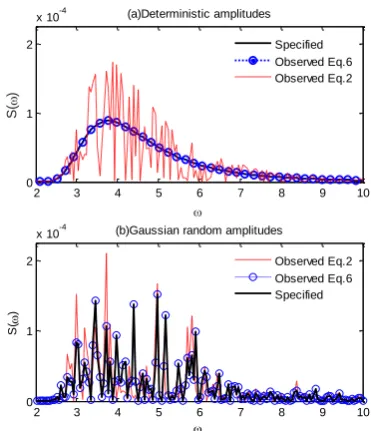
fluctuated due to the random value of _Rn. As a result, the spectrum S'() in the existing approach by Kriebel and Alsina (2000) shows random fluctuations, as demonstrated by the curve marked by ‘Observed (Eq.2) in Fig.1(a), in which a Bretschneider spectrum with significant wave height Hs=0.061m and peak

frequency 0.6Hz, the maximum frequency 2Hz, N=240, xf =15.2m, tf =89s and PT =40% is used

to generate the wave in a water depth of 1.5m. The observed spectra shown in Fig.1a are obtained using the wave time histories of 120s recorded at the expected focusing point by the linear wave theory. The fluctuations here are spurious but not physical.

2.2. Improved approach

In order to embed the rogue waves into random sea, as well as reserve the feature of the specified spectrum without spurious random fluctuations, a correction term is proposed to be introduced in this paper and the new expression of the wave elevation, replacing Eq. (2), becomes,

)

,

(

)

,

(

'

)

,

(

"

x

t



x

t



x

t













c xt A k x t

1 ' cos ) , (    (6b)

Figure 1: Comparison of observed wave spectra at the focusing point and the specified spectrum using linear wave theory (Bretschneider spectrum, d = 1.5m, Hs = 0.061m, peak

frequency 0.6Hz, maximum frequency 2Hz, N=240, xf =15.2m, tf =89s and PT =40% )

) cos( 2 2 2 2 2 Tn Rn Tn Rn Tn Rn Tn Rn C n A A A A A A A        

, (6c)

where '(x,t) is still given by Eq. (2). The spectrum of the waves resulted from Eq. (6a)

corresponding to ωn is





  2 2 2 Tn Rn A A . Therefore,

the observed wave spectrum is identical to the specified spectrumS(). This is confirmed by Fig.1(a). It should be noted that due to the involvement of the correction term _c(x,t)in Eq. 6, the real energy ratio of the random and focusing parts have been changed. PR and PT in

Eq.(6) only provide a reference value for the wave generation.

Tucker et al (1984) pointed out that the use of deterministic amplitudes was not appropriate and might lead to the loss of randomness.

Actually, the amplitudes and the phase



Eq. (2) and Eq. (6) can be determined by using a Gaussian random process as described in Tucker et al (1984) and Taylor et al, (1997).

2 3 4 5 6 7 8 9 10

0 1 2

x 10-4

 S(  ) (a)Deterministic amplitudes Specified Observed Eq.6 Observed Eq.2

2 3 4 5 6 7 8 9 10

0 1 2

x 10-4

S(



)



(b)Gaussian random amplitudes

Fig.1 (b) compares the observed spectra at the focusing point obtained by using Eq. (2), Eq. (6) and the specified spectrum using the method by Tucker et al, (1984) and Taylor et al (1997). As expected, the correction term _c(x,t) in Eq.(6) ensures that the resultant spectrum after assembling the focusing part and the random part is identical to the specified spectrum; whereas the original approach (Eq. 2) by Kriebel and Alsina (2000) leads to a spectrum that is significantly different from the specified one.

3. Summaries of numerical methods

After showing that it is necessary to include the correction terms in Eq. (6), more effects of the correction term will be investigated by numerical tests. As discussed above, significant nonlinearities may be involved following the formation of the rogue waves, especially the second-order ‘bound’ wave leads to set-down and possible set-up of the wave elevation (Adcock and Taylor, 2014; Adcock et al, 2011), which influences the formation of the rogue waves. It is also widely accepted that the nonlinearity of a large transient wave event is not restricted to second order; there are not only bound nonlinearities at third order and above, but also resonant nonlinearities (Gibson and Swan, 2007). According to the knowledge, two numerical methods based on the fully nonlinear theory (FNPT), i.e. the improved SBI (Wang and Ma, 2015) and the QALE-FEM (Ma and Yan, 2006; Yan and Ma, 2010), are employed for the numerical tests on the effects of the correction term. For comparison, the 2nd order wave theory (e.g. Dalzell, 1999; Schäffer, 1996) is also implemented. The details of the FNPT methods can be found in the cited papers. For completeness, the summaries of the improved SBI and QALE-FEM are given herein.

3.2 The Improved SBI method

The improved SBI method is developed based on the original SBI method proposed by Clamond et al (2005), Fructus et al (2005) and Grue (2010). In the SBI, the Neumann operator is introduced and expressed in terms of the free surface and the velocity potential. The kinematic and dynamic boundary conditions are reformulated into the skew-symmetric form after applying the Fourier transform. The free surface and velocity potential are updated through integrating the equations with respect to time, which requires the velocity on the free surface. The velocity on the free surface is decomposed into convolution parts and integration parts. Convolution parts are evaluated by the FFT, and the integration parts have kernels decaying quickly along the distance between the source and field points but their integrands are weakly singular. The distinguishing features of the improved SBI (Wang and Ma, 2015) include (1) a de-singularity technique to accelerate the evaluation of the integrals with weak singularity; (2) an anti-aliasing technique to overcome the aliasing problem associated with Fourier Transform or Inverse Fourier Transform with a limited resolution; and (3) a technique for determining a critical value of the slope of the free surface, under which the integrals can be neglected to further accelerate the computation. In the computational domain of the improved SBI method, a Cartesian coordinate system is selected with the oxy plane on the mean free surface, the x-axis pointing to the right end and the z-axis being positive upwards. The origin of the x-axis locates at the centre of the tank, where a pneumatic wave maker is applied to generate the waves. Damping zones are located at both ends to absorb the progressive waves to prevent the refection. Pre-tests are carried out to make sure that the resolution and time step size are sufficient and no considerable reflected waves are involved.

In the QALE-FEM, the flow is determined by solving a boundary value problem for velocity potential, which satisfies the Laplace’s equation, using a finite element method (FEM). The unstructured computational mesh is moving during the calculation by using a novel methodology based on the spring analogy method but purpose-developed for fully nonlinear water waves including overturning waves. The fully nonlinear free surface conditions are given in arbitrary Lagrangian-Eulerian forms. In addition, this method is also equipped with other purpose-developed techniques: (1) a three-point method or modified SFDI (simplified finite difference interpolation) scheme (Xu et al, 2014) for computing the velocity on the free surfaces; and (2) special technique for coping with wave overturning and impacting. These techniques ensure high robustness of the QALE-FEM. The coordinate system for this method is similar to that used by the improved SBI except the origin of x-axis is located in the left end where there a wavemaker is. The waves are generated by using a wavemaker (piston, flap or hinged) based on either linear or 2nd order wavemaker theory. A numerical wave absorber based on the self-adaptive wavemaker theory (Schäffer and Jakobsen, 2003). Its efficiency has been demonstrated in Ma et al (2015) and will not be discussed here.

3.3 Accuracy

The accuracies of these two numerical methods on modelling fully nonlinear water waves have been demonstrated in our previous publications, e.g. Wang and Ma (2015), Ma and Yan (2006) and Yan and Ma (2010). Necessary comparisons with the experimental results using the cases for extreme waves are presented here to shed light on their accuracies.

(a) Time histories of the wave elevation

(b) Wave spectra

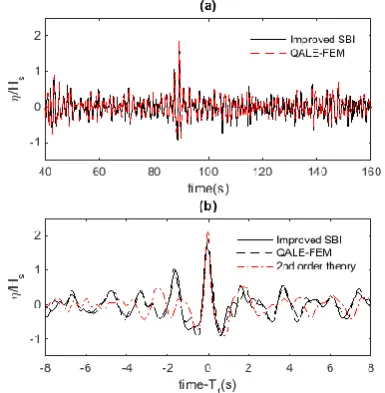
Figure 2: Comparisons between the numerical results and experimental data for (a) the time histories of the wave elevation and (b) the wave spectra recorded at 13.889m from the wave paddle(d = 2.93m, JONSWAP spectrum, Hs =

0.103, peak period of 1.456s)

The experiment was carried out in the 3D wave basin at the Plymouth University. The wave basin is 35 m long and 15.5m wide. The mean water depth (d) used to perform the experiments is 2.93m. Flap wave paddles are installed to generate 3D waves. JONSWAP spectrum with a peak period of 1.456s and significant wave height of 0.103m is used to generate the unidirectional focusing wave using spatial-temporal focusing approach similar to that in Ma (2007). The waves are expected to be focused at 13.886m from the wave paddle. The details of the experiments can be found in Ma et al (2015). Fig. 2(a) shows the time histories of the wave elevation recorded at the expected focusing location. It is clear that both the QALE-FEM and the Improved SBI produce numerical results which agree well with the experimental data. The comparison of the wave spectra displayed in Fig.2(b) also verifies the FFT procedure used in the data analysis for processing the wave spectrum.

The preliminary studies shown above demonstrated that the new technique proposed here ensures that the feature of the specified spectrum can be retained and the spurious fluctuations in the spectrum in the existing techniques (Kriebel and Alsina, 2000) can be removed. In this section, we aim to answer the following questions. (1) How the wave spectrum is affected if not applying the correction in Eq. (6) but just smoothing the spectrum to remove the spurious fluctuations? (2) How does the correction term affect the statistics of maximum wave heights (Hmax)? (3)

How does the nonlinearity affect the wave spectrum? We are aware that some publications have investigated the effects of nonlinearity on the wave spectrum of normal random waves or focusing wave groups (e.g. Baldock et al,1996; Gibson and Swan, 2007; Ning et al, 2009) but no publications looks at the similar questions for rogue waves embedded in a random sea.

Although the preliminary study shown in Fig.1(b) has demonstrated a feasibility of using the improved technique in the Gaussian random process for determining the amplitudes, the deterministic amplitude spectra are employed in the rest of the paper. That is because the use of the deterministic amplitude spectra is sufficient and more convenient to answer the three questions listed above. The wave spectra adopted here are the same as that used in Fig.1, i.e. Bretschneider spectrum with significant wave height Hs=0.061m and peak frequency

0.6Hz. The cut-off high frequency is 2Hz and N = 240, yielding a mean frequency interval of 0.00833Hz. This means that the time history of the wave elevation obtained by linear and 2nd order wave theories behaves periodically with a longest period of 120s. Similar to Fig. 1, xf

=15.2m, tf =89s are specified. The length of

computational domain for the improved SBI is 136m. Because the symmetrical boundary conditions are imposed at the two ends of the domain for the improved SBI, the effective

length is 68m. The length of the computational domain for the QALE-FEM is 30m and a 2nd order piston wavemaker (Schäffer, 1996; Sriram et al, 2013) is installed at the left end and a self-adaptive wavemaker is installed at the other end to absorb the wave. In the fully nonlinear modelling, the initial free surface is the mean free surface (similar to the physical experiments). It takes about 40s for the wave components with highest wave frequency (2Hz) to reach the expected focused location. Based on this, the simulation duration is assigned to be 160s and the time histories at the duration 40~160s are used for the FFT analysis to obtain the wave spectra. Unless mentioned otherwise, all spectra presented in the paper are obtained without implementing any smooth techniques.

4.1Effectiveness of the correction technique

The most essential question (corresponding the first question raised above) to be answered is the effectiveness of the correction term _c(x,t), which forms the basis of the present research. It should be noted that in the theoretical analysis presented in Section 2, xf and tf, are

assigned aiming to achieve a phase coherent of the focusing part at x = xf and t = tf according to

spatial-temporal domain. Therefore, the wave recorded at x = xfmay not represent the maximum wave

in the fully nonlinear simulation. Similar to our previous investigations, e.g. Yan et al (2010, 2011), we concentrate on the location where the maximum wave crest occurs in each case. For simplicity, this is referred to as the real focusing location (Xf), which may be

significantly different from the linear focusing location xf (Ning et al, 2009, Schäffer, 1996;

Sriram et al, 2013). In the same content, the time corresponding to the occurrence of the maximum wave crest is referred to as the real focusing time (Tf).

Figure 3: Wave time histories near the focusing time recorded at x= Xf predicted by different

numerical models using Eq.(6) (PT =20%, Xf =

15.2m and Tf= 89s in the 2

nd

order modelling; Xf = 15.864m and Tf = 89.39s in the fully

nonlinear simulations, respectively)

In the first case considered here, PT =20%. For

the purpose of comparison, the same random series have been used in both the 2nd order and the fully nonlinear simulations when specifying the phase shifts of the random part. It is observed that in the simulations adopting the present technique with correction term, i.e. Eq.(6), Xf = 15.2m and Tf = 89s are predicted

by the 2nd order theory; whereas Xf = 15.864m

and Tf = 89.39s are obtained by both the

improved SBI and the QALE-FEM. The wave time histories recorded at x= Xf are illustrated

in Fig.3. It is clear that the result by the improved SBI agrees well with that by the QALE-FEM.

Figure 4: Wave time histories near the focusing time recorded at x= Xf predicted by different

numerical models using Eq.(2) (PT =20%, Xf =

15.2m and Tf = 89s in the 2

nd

order modelling; Xf = 15.864m and Tf = 89.31s in the fully

nonlinear simulations, respectively)

Similar agreement has also been found in the simulations adopting the original technique without considering the correction term, i.e. Eq. (2), as demonstrated in Fig.4. The relative

errors defined by using 

 

160 40

2 160 40

2 2

dt dt

i q i

  

, in

which the superscripts of ηi and ηq represent the

Figure 5: Wave Spectra recorded at x= Xf in the

cases (PT =20%)

Figure 6: Wave Spectra recorded at the focusing location (PT =20%, numerical results

are obtained by using the improved SBI. Only the spectrum obtained by the original technique (Eq. (2) is smoothed in (b))

The spectra corresponding to the data shown in Figs. 3-4 are presented in Fig.5. From Fig.5 (b), it is clear that by using the original approach, i.e. Eq. (2) without the correction term, the spectra suffer from significant fluctuations, being very different from the originally specified one; whereas the technique using Eq. (6) with the correction term leads to the spectra (Fig.5(a)), which are very close to the specified spectrum. It is clearer in Fig. 6(a), which

compares the spectra obtained using the original technique and the present one by the improved SBI. This is consistent with the linear analysis in Section 2.

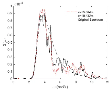
Figure 7: Wave Spectra recorded at x = 5m (numerical results are obtained by using the ESBI)

One may argue that such fluctuations could be artificially removed through smoothing technique as demonstrated in Fig. 6(b), in which only the spectrum from the case adopting the original technique is smoothed 100 times using a five-point smoothing technique (Ma and Yan, 2006). Although the smoothed spectrum seems to be less fluctuated, the analysis on the total spectral energy suggests a significant energy loss at a level of 8% (the total spectral energies obtained by the original technique is 2.33 ×10-4ρg and 2.15×10

-4_{ρg in those shown in Fig.6(a) and Fig.6(b),}

original technique without the correction and the original spectrum may deliver a misleading signal that there is an energy transfer between harmonics due to nonlinearity.

Figure 8: Wave Spectra recorded at the focusing location in the cases with different PT

(numerical results are obtained by using the improved SBI)

Similar phenomena are also found in the cases with other values of PT ranging from 40% to

80%. The wave spectra recorded at the focusing location in the cases with different values of PT

are illustrated in Fig.8. For clarity, only the numerical results by the improved SBI are presented. Again, the effectiveness of the correction term on retaining the features of the specified spectrum without suffering from significant fluctuations in the spectrum is confirmed within the entire range of the investigations.

One may also notice that minor fluctuations are detected in the spectra obtained by the present technique in Fig. 6 and Fig.8. Such minor

fluctuations are caused by the nonlinearity, as evidenced in Fig. 7 that shows a consistent smoothed spectrum obtained using the present technique at the location where the nonlinearity is not significant. Similar observation is also confirmed experimentally for focusing waves without random waves. More discussions on the nonlinear behaviour of spectral development in the cases with a rogue wave embedded in random waves will be given in the following section.

4.2 Nonlinear effects on wave spectra

In the results presented above, some nonlinear effects have been revealed. In this section, it will be discussed in more details. Many researchers have explored nonlinear evolution of the wave spectra in the cases with focusing wave groups, e.g. Baldock et al, (1996) and Ning et al, (2009), without the background random waves. They concluded that the nonlinearity transfers the wave energy to both lower and higher harmonics. However, no publication looks at the similar issue for rogue waves embedded in random seas. Due to the significant fluctuation of the spectra and/or considerable energy loss if smoothing the spectra in the cases adopting the original technique, we address this issue by using the present technique with the correction term for generating waves.

direction of the propagation, which are illustrated in Fig. 9 for the cases with PT =60%

and PT =80%. As can be seen, near the

wavemaker, e.g. x=5m, the wave spectrum is close to the specified one. The spectrum within the range around 4-7 rad/s become lower and the wave energy in higher harmonics, i.e. ω>7rad/s, becomes more significant, as the distance from the wavemaker becomes longer until the focusing location, i.e. 15.864m, following the occurrence of the rogue waves. The numerical results also reveal that after the focusing location, the spectral energy seems to transfer from the higher harmonics back to the fundamental harmonics as evidenced in Fig. 10, which illustrates the spectra recorded at different locations including the one after the focusing point in the case with PT = 80%. This

observation is very similar to the existing publications on the focusing wave groups without the random background.

Figure 9: Spectra recorded at different locations with different values of PT (numerical results

are obtained by using the improved SBI)

Figure 10: Spectra recorded at different locations with PT = 80% (numerical results are

obtained by using the improved SBI)

Figure 11: Spectra recorded at focusing location with different PT (numerical results are

obtained by using the improved SBI)

What is more interesting here is how the random part affects the nonlinear behaviour of the spectral development. For this purpose, Fig.11 is presented, which compares the spectra at focusing location in the cases with different PT. From this figure, it is clear that the wave

spectrum at higher harmonics, e.g. ω>7rad/s, increases considerably (evidencing more wave energy is transferred to higher harmonics) as PT

increases, although the difference between the case with PT =60% and PT =80% is less

significant. Additionally, the difference between the case with PT =80% and other cases

with lower PT values is that the spectral energy

to lower and higher harmonics as PT increases,

as more wave energy are expected to be focused at the focusing location leading to much higher wave steepness and thus stronger nonlinearity.

The discussions following Figs. 8-11 show a significant nonlinearity associated with the rogue waves embedded in the random waves. However, in the design practices, the 2nd order wave theory is very popular for random sea analysis. Experiments have confirmed that it may be inadequate for modelling focusing waves under extreme sea states (Ning et al, 2009, Gibson and Swan, 2007). Nevertheless, due to the split of the wave energy discussed in this paper, the expected rogue waves may have lower degree of nonlinearity than the fully focusing wave with the same spectrum. From Figs.3-4 for the cases with PT =20%, it is found

that the 2nd order predictions on the wave time histories seem to be different from the fully nonlinear results, however, the maximum wave height observed is very close. The spectral results shown in Fig.5 also confirm a good agreement between the 2nd order results and the fully nonlinear predictions. This implies that 2nd order theory may be applied to such cases with acceptable accuracy. However, with the increases of the PT, the wave height increases,

so does the local wave steepness. The 2nd order wave theory may not give acceptable predictions. Therefore, the suitability of the 2nd order theory may need to be assessed. This is related to the Question (3) stated in the beginning of this section. We are not trying to fully address this issue but to shed some light on the suitability of the 2nd order theory on modelling rogue waves embedded in the random waves. Two specific parameters, i.e. the maximum wave height and the wave spectrum are concentrated. Other nonlinear features for rogue waves, such as the low frequency set-down/set-up (Adcock and Taylor, 2014) and the local steepness related to the

wave breaking are also of interest, but they will be discussed in future.

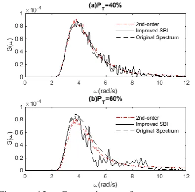
Figure 12: Comparison of wave spectra recorded at focusing location between the improved SBI and the 2nd order wave theory (Eq.(6) is used to generate the waves)

Fig. 12 compares the wave spectrum at the focusing location obtained by using the improved SBI with that obtained by using the 2nd order wave theory. The present technique with the correction term, i.e., Eq.(6), is employed to generate waves. As pointed out by Janssen (2009), the main effect from the second order is a shift of the low-frequency part of the wave spectrum towards higher frequencies, while at high frequencies there is an increase in spectral levels. This is confirmed again by Fig. 12, in which the evolution of the spectrum obtained by using both the second order wave model and the improved SBI is consistent with Janssen’s conclusion. Meanwhile, it is clear that with PT =40%

(Fig.12(a)), the 2nd order result is fairly close to the fully nonlinear results; but their results are significantly different when PT=60% (the 2

nd

Figure 13: Comparison of maximum wave height recorded at focusing location between the improved SBI and the 2nd order wave theory

Consideration is also made to the maximum wave heights (Hmax) in the cases with different

values of PT. Some results are shown in Fig.13.

It confirms that the results of different methods are very close when PT = 20%. As expected,

with increase in PT, the difference between the

improved SBI and the 2nd order theory becomes more significant. It is also interesting to see that Hmax obtained by the 2

nd

order are higher than that by the fully nonlinear simulation for PT > 20%.

It is also found from Fig.13 that for higher values of PT, i.e. ≥60%, the maximum wave

heights obtained by using the original technique and the present one are quite close. This is because the random wave energy takes lower percentage of energy, and so the correction term in Eq. (6) becomes small in these cases. Based on the results shown in Figs. 12-13, one may agree that for the specific wave condition, the 2nd order wave theory may be considered to be acceptable for PT < 40% in term of

maximum wave heights. However, it shall be noted that the validity of the 2nd order wave theory may also be affected by other parameters such as the local wave steepness of the rogue wave. The threshold value 40% may only be suitable for the specific wave spectrum and condition discussed here.

4.3Statistics of Hmax and ηmax

In the experiments by Kriebel and Alsina (2000), who adopted Eq. (2) to generate the waves without considering the correction term,

some results for the statistics of Hmax and ηmax

with different values of PT are discussed. In

this section, we will look at how the correction term affects the statistical values of Hmax and

ηmax. To do so, 100 cases with different random

series but the same value of PT are investigated

using the 2nd order wave theory.

Figure 14: Probability density of the maximum wave height recorded at x=xf. using 2

nd

order wave theory

Fig.14 displays the probability density of the maximum wave height recorded at the linear focusing location xf.. Both the original

technique of Kriebel and Alsina (2000) without the correction term and the present technique with the correction term are used for comparison. As can be seen in Fig.14, the maximum wave heights (Hmax) show a

significant difference between the results for the original and the present techniques. Within 100 samples, the difference may reach to 2.5~3 Hs. It is noted that the experimental results

obtained by Kriebel and Alsina (2000), i.e. 2.21 and 2.48Hs corresponding to PT =15% and 20%,

respectively, are within the range shown in Fig.14(b). The corresponding probability densities are 0.78 and 0.68, respectively. As can be seen, if the original technique without correction (Eq.(2)) is used, most probable Hmax

continuously increases with the increase of PT.

correction (Eq.(6)), the most probable Hmax does

not change significantly for smaller value of PT ,

e.g. ≤20%, but increases with further increases of PT from 30%. The direct comparison

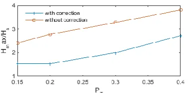
between the results obtained by using the two techniques is given in Fig.15. From this figure it appears that without the correction term, the most probable maximum wave heights are significantly overestimated, by approximately 1.2Hs.

Figure 15: Comparison of most probable Hmax

recorded at x=xf. (2

nd

order wave theory, 100 individual case studies)

5. Conclusions

In this paper, an improved technique for generating rogue waves in random sea using the method of Kribel and Alsina (2000) is suggested with introducing a correction term. The effectiveness of the proposed technique is investigated by numerical tests using the 2nd order wave theory, and the QALE-FEM and the improved SBI methods based on FNPT. The investigations suggest that the improved. The investigations suggest that the improved technique effectively retain the features of the specified wave spectrum and remove spurious fluctuations in the existing method. The statistical studies on the most probable maximum wave heights indicate that the original technique without the correction term can artificially over-predict the probability of the occurrence of the maximum wave heights for a given wave spectrum.

This paper has focused on the 2D problems but the technique can be extended to model 3D

crossing random sea state. The relevant work will be left to future publications.

Acknowledgement: The authors acknowledge the financial support from the ESPRC, UK (EP/L01467X/1). The first author is supported by the Chinese Scholarship Council (PhD program No. 2011633117), to which the author is most grateful.

Reference

Adcock, T.A.A.; Taylor, P.H.(2014): The physics of anomalous (‘rogue’) ocean waves, Reports on Progress in Physics, Vol. 77, 105901.

Adcock, T.A.A.; Taylor, P.H.; Yan, S.; Ma, Q.W.; Janssen, P.A.E.M.,(2011): Did the Draupner wave occur in a crossing sea? Proceeding of the royal society A, 467(2134), 3004-3021.

Adcock, T.A.A.; Yan, S., (2010): The focusing of uni-directional Gaussian wave-groups: An

approximate NLSE based approach,

Proceeding of 29th International Conference on Ocean, Offshore and Arctic Engineering, Shanghai, China, Vol. 4, 569-576.

Baldock, T. E.; Swan, C.; Taylor, P. H.,

(1996): A Laboratory Study of Nonlinear Surface Waves on Water. Philosophical Transactions of the Royal Society A, 354(1707), 649–676.

Clamond, D.; Fructus, D.; Grue, J.; Kristiansen O., (2005): An efficient model for three-dimensional surface wave simulations. Part II: Generation and absorption," Journal of Computational Physics, Vols. 205: 686-705.

Clauss, G.F.; Steinhagen, U., (2000): Optimization of Transient Design Waves in Random Sea, Proceedings of the Tenth(2000) International Offshore and Polar Engineering Conference, Seattle, USA, Vol. 3, 229-236.

Dalzell, J.F., (1999): A note on finite depth second-order wave-wave interactions, Applied Ocean Research, Vol. 21,105-111.

theory. Journal of Physical Oceanography, Vol. 30, 1931–1943.

Fructus, D.; Clamond, D.; Grue, J.; Kristiansen, O., (2005): An efficient model for three-dimensional surface wave simulations Part I: Free space problems, Journal of Computational Physics, Vols. 205, 665-685.

Funke, E.R.; Mansard, E.P.D, (1982): The control of wave asymmetries in random waves, Proceeding of 18th International Conference on Coastal Engineering, Cape Town, South Africa, 725-744.

Gibson, R.S, Swan, C, (2007): The evolution of large ocean waves:the role of local and rapid spectral changes, Proceedings of the Royal Society A,Vol.463,21-48

Grue, J, (2010): Computation formulas by FFT of the nonlinear orbital velocity in three-dimensional surface wave fields, Journal of Engineering Mathematics., Vol. 67, 55-69

Janssen, P. A. M., (2009): On some consequences of the canonical transformation in the Hamiltonian theory of water waves. Journal of Fluid Mechanics, Vol. 637, 1-44.

Johannessen, T. B., & Swan, C. (2001). A laboratory study of the focusing of transient and directionally spread surface water waves. Proceedings of the Royal Society of London A: Mathematical, Physical and Engineering Sciences, Vol. 457, No. 2008, pp. 971-1006.

Kim, C.H.,(2008):Nonlinear Waves and Offshore Structure, Singapore: World Scientific Publishing Co. Pte. Ltd.

Kharif, C.; Pelinovsky, E., (2003): Physical mechanisms of the rogue wave phenomenon. European Journal Mechanics B / Fluid, Vol. 22, 603-634.

Kharif, C; Pelinovsky, E.,(2009): Rogue Waves in the Ocean, Berlin Heidelberg, Springer-Verlag.

Kriebel, D. L.; Alsina, M. V.,(2000): Simulation of Extreme Waves in a Background Random Sea, Proceedings of the Tenth(2000) International Offshore and Polar Engineering Conference, Vol. 3, 31-37.

Lindgren, G. (1970): Some properties of a normal process near a local maximum, The Annals of Mathematical Statistics, Vol. 41(6), 1870-1883.

Liu, P.C.; Pinho, U.F., (2004): Freak waves— More frequent than rare! Annual Geophysics, Vol. 22(5), 1839– 1842.

Ma, Q.W. (2007): Numerical generation of freak waves using MLPG_R and QALE-FEM methods. CMES: Computer Modeling in Engineering & Sciences, Vol. 18(3), 223-234.

Ma, Q.W.; Yan, S.,(2006): Quasi ALE finite element method for nonlinear water waves, Journal of Computational Physics. Vol. 212, 52-72.

Ma, Q.W.; Yan, S.; Greaves, D., Mai, T., Raby, A.,(2015): Numerical and experimental studies of interaction between FPSO and focusing waves, submitted to the 25th (2015) International Offshore and Polar Engineering Conference , Kona, USA.

Ning, D.Z.; Zang, J.; Liu, S.X.; Eatock Taylor, R.; Teng, B.; Taylor, P., (2009): Free-surface evolution and wave kinematics for nonlinear uni-directional focused wave groups, Ocean Engineering, Vol. 36,1226–1243.

Schäffer, H.A.,(1996): Second order wavemaker theory for irregular waves, Ocean Engineering, Vol. 23(1), 47-88.

Schäffer, H.A.; Jakobsen, K.P., (2003): Nonlinear wave generation and active absorption in wave flumes, Proceeding of Long Wave Symposium, 2003, Thessaloniki, Greece.

Skourup, J.; Ottensen Hansen, N.; Andreasen, K., (1996): Non-Gaussian Extreme Waves in the Central North Sea, Proc. Offshore Mechanics and Arctic Engineering Conf., Vol. I-A, 25-32.

Sriram, V.; Schlurmann, T.; Schimmels, S.,

Taylor, P. H., Jonathan, P., & Harland, L. A.

(1997). Time domain simulation of jack-up dynamics with the extremes of a Gaussian

process. Journal of vibration and

acoustics, Vol. 119(4), 624-628.

Touboul, J.; Giovanangeli, J.P.; Kharif, C.; Pelinovsky, E.,(2006): Freak waves under the action of wind: experiments and simulations, European Journal Mechanics B / Fluid ,Vol. 25, 662–676.

Touboul, J.; Pelinovsky, E.; Kharif, C.(2007): Nonlinear focusing wave group on current. Journal of Korean Society of Coastal and Ocean Engineers, Vol.19,222-227.

Tucker MJ Challenor PG Carter, DJT

(1984): Numerical simulation of a random sea: a common error and its effect upon wave group statistics. Applied Ocean Research, Vol.6 (2), 118–122.

Walker, D.A.G.; Taylor, P.H.;. Eatock Taylor, R.,(2005): The shape of large surface waves on the open sea and the Draupner New Year wave. Apply Ocean Research, Vol. 26, 73–83.

Wang, J.; Ma, Q.W., (2015): Numerical techniques on improving computational efficiency of Spectral Boundary Integral Method. International Journal for Numerical Methods in Engineering. Vol. 102(10), 1638-1669.

Wu, C.H.; Yao, A.,(2004): Laboratory measurements of limiting freak waves on current. Journal of Geophysical Research, 109:C12002, dio:10.1029/2004JC002612.

Xu, G.; Yan, S.; Ma, Q.W.,(2014): Modified SFDI for fully nonlinear wave simulation, accepted to be published in CMES: Computer Modeling in Engineering & Sciences.

Yan, S.; Ma, Q.W.,(2010a): QALE-FEM for modelling 3D overturning waves, International Journal for Numerical Methods in Fluids, Vol. 63, 743-768.

Yan, S.; Ma, Q.W.,(2010b): Numerical simulation of interaction between wind and 2D freak waves, European Journal Mechanics B / Fluid ,Vol. 29, 18–31.

Yan, S.; Ma, Q.W., Adcock, T.A.A, (2010): Investigation of freak waves on uniform current, Proceeding of 25th international workshop on water waves and floating bodies, Harbin, China.

Yan, S.; Ma, Q.W.,(2011): Improved model for air pressure due to wind on 2D freak waves in finite depth, European Journal Mechanics B / Fluid ,Vol. 30, 1–11.