Deterministic numerical modelling of three-dimensional rogue waves on large scale with presence of wind

City, University of London Institutional Repository

Citation

:

Wang, J., Yan, S. & Ma, Q. (2018). Deterministic numerical modelling of

three-dimensional rogue waves on large scale with presence of wind. Procedia IUTAM, 26, pp.

214-226. doi: 10.1016/j.piutam.2018.03.021

This is the published version of the paper.

This version of the publication may differ from the final published

version.

Permanent repository link:

http://openaccess.city.ac.uk/20013/

Link to published version

:

http://dx.doi.org/10.1016/j.piutam.2018.03.021

Copyright and reuse:

City Research Online aims to make research

outputs of City, University of London available to a wider audience.

Copyright and Moral Rights remain with the author(s) and/or copyright

holders. URLs from City Research Online may be freely distributed and

linked to.

ScienceDirect

Available online at Available online at www.sciencedirect.comwww.sciencedirect.com

Procedia IUTAM 00 (2017) 000–000

www.elsevier.com/locate/procedia

2210-9838 © 2017 The Authors. Published by Elsevier B.V.

Selection and peer-review under responsibility of IUTAM Symposium on Storm Surge Modelling and Forecasting.

IUTAM Symposium on Storm Surge Modelling and Forecasting

Storm surge prediction: present status and future challenges

Jiachun Li

_{*, Bingchuan Nie}

a_{Key Laboratory for Mechanics in Fluid Solid Coupling Systems, Institute of Mechanics, Chinese Academy of Sciences, Beijing, 100190, China.} b_{School of Engineering Science, University of Chinese Academy of Sciences, Beijing 100049, China.}

c_{School of Civil Engineering, Beijing Jiaotong University, Beijing 100044, China.}

Abstract

In the current review, the most pessimistic events of the globe in history are addressed when we present severe impacts caused by storm surges. During previous decades, great progresses in storm surge modeling have been made. As a result, people have developed a number of numerical software such as SPLASH, SLOSH etc. and implemented routine operational forecast by virtue of powerful supercomputers with the help of meteorological satellites and sensors as verification tools. However, storm surge as a killer from the sea is still threatening human being and exerting enormous impacts on human society due to economic growth, population increase and fast urbanization. To mitigate the effects of storm surge hazards, integrated research on disaster risk (IRDR) as an ICSU program is put on agenda. The most challenging issues concerned such as

abrupt variation in TC’s track and intensity, comprehensive study on the consequences of storm surge and the effects of climate change on risk estimation are emphasized. In addition, it is of paramount importance for coastal developing countries to set up forecast and warning system and reduce vulnerability of affected areas.

© 2016 The Authors. Published by Elsevier B.V.

Selection and peer-review under responsibility of IUTAM Symposium on Storm Surge Modelling and Forecasting.

Keywords: Storm surge, Tropical cyclone; Extratropical cyclone; SPLASH, SLOSH; Risk analysis; IRDR

1.Introduction

Storm surge, an extraordinary sea surface elevation induced by atmospheric disturbance (wind and atmospheric pressure), is regarded as a most catastrophic natural disaster. According to long term statistical analysis, total death toll amounted to 1.5 million and property losses exceeded hundred billions USD globally since 18751_{. They could}

* Corresponding author. Tel.: +86-010-8254-4203; fax: +86-010-6256-0914

E-mail address: [email protected]

www.elsevier.com/locate/procedia Procedia IUTAM 26 (2018) 214–226

2210-9838 © 2018 The Authors. Published by Elsevier B.V.

Peer-review under responsibility of the scientific committee of the IUTAM Symposium Wind Waves. 10.1016/j.piutam.2018.03.021

10.1016/j.piutam.2018.03.021 2210-9838

© 2018 The Authors. Published by Elsevier B.V.

Peer-review under responsibility of the scientific committee of the IUTAM Symposium Wind Waves.

ScienceDirect

Procedia IUTAM 00 (2018) 000–000

www.elsevier.com/locate/procedia

2210-9838 © 2018 The Authors. Published by Elsevier B.V.

Peer-review under responsibility of the scientific committee of the IUTAM Symposium Wind Waves.

IUTAM Symposium Wind Waves, 4–8 September 2017, London, UK

Deterministic numerical modelling of three-dimensional rogue

waves on large scale with presence of wind

Jinghua Wang

_{, Shiqiang Yan}

_{*, Qingwei Ma}

a_{City University of London, Northampton Square, London, EC1V 0HB, United Kingdom}

Abstract

Oceanic rogue waves are a subject of great interest and can cause devastating consequences. Rogue waves are abnormal in that they stand out from the waves that surround them. Rogue waves are often observed accompanied by high wind in reality, and some earlier studies have demonstrated that the energy input due to the wind can enhance the dynamics of the rogue waves, which further causes huge concern about the safety of the human’s oceanic activities. Thus it is important, to better understand the mechanisms between the wind-wave interactions and to study the rogue waves with the presence of wind, especially on a three-dimensional large scale. In this study, numerical simulations are performed by using the Enhanced Spectral Boundary Integral (ESBI) method based on the fully nonlinear potential theory, in order to investigate the effects of wind on the rogue waves. The wind effects are introduced by imposing a wind-driven pressure on the free surface, which is empirically formulated based on intensive numerical investigation using multiple-phase Navier-Stokes solver. The results of the simulation confirm that the presented ESBI can produce satisfactory results on the formation of rogue waves under the action of wind. It provides a foresight of modelling rogue waves with presence of wind on a large scale in a phase-resolved fashion, which may motivate relevant studies in the future.

© 2018 The Authors. Published by Elsevier B.V.

Peer-review under responsibility of the scientific committee of the IUTAM Symposium Wind Waves.

Keywords: Freak wave; Fully nonlinear potential theory; Focusing wave; Spreading sea.

* Corresponding author. Tel.: +44 (0)20 7040 3330. E-mail address: [email protected]

ScienceDirect

www.elsevier.com/locate/procedia

2210-9838 © 2018 The Authors. Published by Elsevier B.V.

Peer-review under responsibility of the scientific committee of the IUTAM Symposium Wind Waves.

IUTAM Symposium Wind Waves, 4–8 September 2017, London, UK

Deterministic numerical modelling of three-dimensional rogue

waves on large scale with presence of wind

Jinghua Wang

_{, Shiqiang Yan}

_{*, Qingwei Ma}

a_{City University of London, Northampton Square, London, EC1V 0HB, United Kingdom}

Abstract

Oceanic rogue waves are a subject of great interest and can cause devastating consequences. Rogue waves are abnormal in that they stand out from the waves that surround them. Rogue waves are often observed accompanied by high wind in reality, and some earlier studies have demonstrated that the energy input due to the wind can enhance the dynamics of the rogue waves, which further causes huge concern about the safety of the human’s oceanic activities. Thus it is important, to better understand the mechanisms between the wind-wave interactions and to study the rogue waves with the presence of wind, especially on a three-dimensional large scale. In this study, numerical simulations are performed by using the Enhanced Spectral Boundary Integral (ESBI) method based on the fully nonlinear potential theory, in order to investigate the effects of wind on the rogue waves. The wind effects are introduced by imposing a wind-driven pressure on the free surface, which is empirically formulated based on intensive numerical investigation using multiple-phase Navier-Stokes solver. The results of the simulation confirm that the presented ESBI can produce satisfactory results on the formation of rogue waves under the action of wind. It provides a foresight of modelling rogue waves with presence of wind on a large scale in a phase-resolved fashion, which may motivate relevant studies in the future.

© 2018 The Authors. Published by Elsevier B.V.

Peer-review under responsibility of the scientific committee of the IUTAM Symposium Wind Waves.

Keywords: Freak wave; Fully nonlinear potential theory; Focusing wave; Spreading sea.

* Corresponding author. Tel.: +44 (0)20 7040 3330. E-mail address: [email protected]

2 Wang, et al./ Procedia IUTAM 00 (2018) 000–000

1.Introduction

Rogue waves in the ocean are extreme waves with a maximum height larger than twice the significant wave height (Hs) and/or crest larger than 1.2Hs [1]. Studies on rogue waves have attracted extensive attentions from the community of engineers and applied scientists over the last few decades. They have been recognized as great threats to marine structures, whereas possible causes resulting their formation can be due to the spatial-temporal focusing, the instability of nonlinear Stokes waves, wave-topography or wave-current interactions, etc. Good reviews of rogue waves are given by Kharif, et al. [1] and Adcock & Taylor [2].

In addition, another factor that cannot be overlooked accounting for rogue wave occurrence is due to the presence of wind according to in-situ observation [3]. However, the question about how rogue waves are generated and/or influenced by wind cannot be completely understood at present. In general, there are two ways to study rogue waves: statistical and deterministic approaches (see discussion in second paragraph of Adcock et al. [31]). The former provides very useful information about the probability of rogue wave occurrence or the wave spectra, contributing to the wave forecasting and hindcasting. Nevertheless, the dynamic features of the waves are important as well and can only be obtained by the latter. To examine the mechanism of energy transferring from wind to waves, deterministic approaches are more straightforward and thus preferred. For example, investigations on wind effects on the rogue wave dynamics have been reported by Giovanangeli, et al. [4], Touboul, et al. [5], Kharif, et al. [6], Yan & Ma [7-9], etc., where it has been demonstrated that wind may dramatically affect the properties of two-dimensional rogue waves. More recently, studies about the effects of wind on rogue waves have been carried out in both laboratory [10-15] and numerical simulations [16-18], which provides significant insights for better understanding the mechanism between wind-wave interactions.

For numerically simulating the interaction between wind and waves, Yan and Ma [7] summarised four existing numerical strategies, in terms of how the wind flow is coupled with the waves. These include (1) a single-phase Navier-Stokes equation to model the air flow, whilst the waves are represented by a pre-described wavy surface [26-30]; (2) the fully nonlinear potential theory (FNPT) models the water waves, in which a wind-excited pressure term imposed on free surface [5-6]; (3) a two-phase Navier-Stokes model to model the air and water flow simultaneously [18]; and (4) a hybrid model combining Strategy 3 and 4 [7,16]. Strategy 1 primarily focuses on the air flow pattern on the pre-described wavy surface and provide useful information on vortex shedding and turbulence near the wavy surface. However, it cannot contribute to the question how the waves are influenced by the air flow. Theoretically, Strategy 3 and 4 can fully couple the air flow and wave motions and, thus, consider the effects of wind on wave field as well as the feedback from the waves to the wind field, the drawback is their low computational efficiency, which is prohibitive especially for large-scale three-dimensional simulations. This paper adopts Strategy 2 with focus on the evolution of waves rather than the variation of the wind field. The FNPT model with external forcing terms to represent the wind-driven pressure on the free surface is applied, following the work done by Touboul, et al. [5], Kharif, et al. [6] and Yan & Ma [9], who have successfully applied the strategy to investigate wind effects on 2D rogue waves generated by using temporal-spatial focus mechanism. However, according to Xiao, et al. [19], to study the weakly non-linear effects which may contribute to rogue waves, the spatial and temporal scale should be commensurate with those of quartet wave-wave interaction. This allows the effect of the Benjamin-Feir like instabilities (see section 4.3 in Janssen [32]), i.e., 𝐿𝐿/𝐿𝐿!, 𝑇𝑇/𝑇𝑇!~𝑂𝑂 𝜀𝜀!! , where 𝐿𝐿! and 𝑇𝑇! are the peak wave length and peak period, respectively, 𝜀𝜀 is the wave steepness. Whereas for regional statistics of rogue waves in spreading seas, those scales should be applied to determine the domain size and duration of three dimensional simulations. Though two-dimensional rogue waves considering the wind effects in local area have been discussed in previous studies, investigation on the wind acting on three-dimensional rogue waves in large scale spreading seas is rare. Nevertheless, the nonlinear effects on transversal direction cannot be overlooked. For instance, the soliton envelope as one of the rogue wave prototype, is found to be transversally unstable, which requires consideration of the transverse wave direction [1]. Therefore, in this paper we focus on the wind effects on three-dimensional rogue waves.

Jinghua Wang et al. / Procedia IUTAM 26 (2018) 214–226 215 Available online at www.sciencedirect.com

ScienceDirect

www.elsevier.com/locate/procedia

2210-9838 © 2018 The Authors. Published by Elsevier B.V.

Peer-review under responsibility of the scientific committee of the IUTAM Symposium Wind Waves.

IUTAM Symposium Wind Waves, 4–8 September 2017, London, UK

Deterministic numerical modelling of three-dimensional rogue

waves on large scale with presence of wind

Jinghua Wang

_{, Shiqiang Yan}

_{*, Qingwei Ma}

a_{City University of London, Northampton Square, London, EC1V 0HB, United Kingdom}

Abstract

Oceanic rogue waves are a subject of great interest and can cause devastating consequences. Rogue waves are abnormal in that they stand out from the waves that surround them. Rogue waves are often observed accompanied by high wind in reality, and some earlier studies have demonstrated that the energy input due to the wind can enhance the dynamics of the rogue waves, which further causes huge concern about the safety of the human’s oceanic activities. Thus it is important, to better understand the mechanisms between the wind-wave interactions and to study the rogue waves with the presence of wind, especially on a three-dimensional large scale. In this study, numerical simulations are performed by using the Enhanced Spectral Boundary Integral (ESBI) method based on the fully nonlinear potential theory, in order to investigate the effects of wind on the rogue waves. The wind effects are introduced by imposing a wind-driven pressure on the free surface, which is empirically formulated based on intensive numerical investigation using multiple-phase Navier-Stokes solver. The results of the simulation confirm that the presented ESBI can produce satisfactory results on the formation of rogue waves under the action of wind. It provides a foresight of modelling rogue waves with presence of wind on a large scale in a phase-resolved fashion, which may motivate relevant studies in the future.

© 2018 The Authors. Published by Elsevier B.V.

Peer-review under responsibility of the scientific committee of the IUTAM Symposium Wind Waves.

Keywords: Freak wave; Fully nonlinear potential theory; Focusing wave; Spreading sea.

* Corresponding author. Tel.: +44 (0)20 7040 3330. E-mail address: [email protected]

Available online at www.sciencedirect.com

ScienceDirect

www.elsevier.com/locate/procedia

2210-9838 © 2018 The Authors. Published by Elsevier B.V.

Peer-review under responsibility of the scientific committee of the IUTAM Symposium Wind Waves.

IUTAM Symposium Wind Waves, 4–8 September 2017, London, UK

Deterministic numerical modelling of three-dimensional rogue

waves on large scale with presence of wind

Jinghua Wang

_{, Shiqiang Yan}

_{*, Qingwei Ma}

a_{City University of London, Northampton Square, London, EC1V 0HB, United Kingdom}

Abstract

Oceanic rogue waves are a subject of great interest and can cause devastating consequences. Rogue waves are abnormal in that they stand out from the waves that surround them. Rogue waves are often observed accompanied by high wind in reality, and some earlier studies have demonstrated that the energy input due to the wind can enhance the dynamics of the rogue waves, which further causes huge concern about the safety of the human’s oceanic activities. Thus it is important, to better understand the mechanisms between the wind-wave interactions and to study the rogue waves with the presence of wind, especially on a three-dimensional large scale. In this study, numerical simulations are performed by using the Enhanced Spectral Boundary Integral (ESBI) method based on the fully nonlinear potential theory, in order to investigate the effects of wind on the rogue waves. The wind effects are introduced by imposing a wind-driven pressure on the free surface, which is empirically formulated based on intensive numerical investigation using multiple-phase Navier-Stokes solver. The results of the simulation confirm that the presented ESBI can produce satisfactory results on the formation of rogue waves under the action of wind. It provides a foresight of modelling rogue waves with presence of wind on a large scale in a phase-resolved fashion, which may motivate relevant studies in the future.

© 2018 The Authors. Published by Elsevier B.V.

Peer-review under responsibility of the scientific committee of the IUTAM Symposium Wind Waves.

Keywords: Freak wave; Fully nonlinear potential theory; Focusing wave; Spreading sea.

* Corresponding author. Tel.: +44 (0)20 7040 3330. E-mail address: [email protected]

2 Wang, et al./ Procedia IUTAM 00 (2018) 000–000

1.Introduction

Rogue waves in the ocean are extreme waves with a maximum height larger than twice the significant wave height (Hs) and/or crest larger than 1.2Hs [1]. Studies on rogue waves have attracted extensive attentions from the community of engineers and applied scientists over the last few decades. They have been recognized as great threats to marine structures, whereas possible causes resulting their formation can be due to the spatial-temporal focusing, the instability of nonlinear Stokes waves, wave-topography or wave-current interactions, etc. Good reviews of rogue waves are given by Kharif, et al. [1] and Adcock & Taylor [2].

In addition, another factor that cannot be overlooked accounting for rogue wave occurrence is due to the presence of wind according to in-situ observation [3]. However, the question about how rogue waves are generated and/or influenced by wind cannot be completely understood at present. In general, there are two ways to study rogue waves: statistical and deterministic approaches (see discussion in second paragraph of Adcock et al. [31]). The former provides very useful information about the probability of rogue wave occurrence or the wave spectra, contributing to the wave forecasting and hindcasting. Nevertheless, the dynamic features of the waves are important as well and can only be obtained by the latter. To examine the mechanism of energy transferring from wind to waves, deterministic approaches are more straightforward and thus preferred. For example, investigations on wind effects on the rogue wave dynamics have been reported by Giovanangeli, et al. [4], Touboul, et al. [5], Kharif, et al. [6], Yan & Ma [7-9], etc., where it has been demonstrated that wind may dramatically affect the properties of two-dimensional rogue waves. More recently, studies about the effects of wind on rogue waves have been carried out in both laboratory [10-15] and numerical simulations [16-18], which provides significant insights for better understanding the mechanism between wind-wave interactions.

For numerically simulating the interaction between wind and waves, Yan and Ma [7] summarised four existing numerical strategies, in terms of how the wind flow is coupled with the waves. These include (1) a single-phase Navier-Stokes equation to model the air flow, whilst the waves are represented by a pre-described wavy surface [26-30]; (2) the fully nonlinear potential theory (FNPT) models the water waves, in which a wind-excited pressure term imposed on free surface [5-6]; (3) a two-phase Navier-Stokes model to model the air and water flow simultaneously [18]; and (4) a hybrid model combining Strategy 3 and 4 [7,16]. Strategy 1 primarily focuses on the air flow pattern on the pre-described wavy surface and provide useful information on vortex shedding and turbulence near the wavy surface. However, it cannot contribute to the question how the waves are influenced by the air flow. Theoretically, Strategy 3 and 4 can fully couple the air flow and wave motions and, thus, consider the effects of wind on wave field as well as the feedback from the waves to the wind field, the drawback is their low computational efficiency, which is prohibitive especially for large-scale three-dimensional simulations. This paper adopts Strategy 2 with focus on the evolution of waves rather than the variation of the wind field. The FNPT model with external forcing terms to represent the wind-driven pressure on the free surface is applied, following the work done by Touboul, et al. [5], Kharif, et al. [6] and Yan & Ma [9], who have successfully applied the strategy to investigate wind effects on 2D rogue waves generated by using temporal-spatial focus mechanism. However, according to Xiao, et al. [19], to study the weakly non-linear effects which may contribute to rogue waves, the spatial and temporal scale should be commensurate with those of quartet wave-wave interaction. This allows the effect of the Benjamin-Feir like instabilities (see section 4.3 in Janssen [32]), i.e., 𝐿𝐿/𝐿𝐿!, 𝑇𝑇/𝑇𝑇!~𝑂𝑂 𝜀𝜀!! , where 𝐿𝐿! and 𝑇𝑇! are the peak wave length and peak period, respectively, 𝜀𝜀 is the wave steepness. Whereas for regional statistics of rogue waves in spreading seas, those scales should be applied to determine the domain size and duration of three dimensional simulations. Though two-dimensional rogue waves considering the wind effects in local area have been discussed in previous studies, investigation on the wind acting on three-dimensional rogue waves in large scale spreading seas is rare. Nevertheless, the nonlinear effects on transversal direction cannot be overlooked. For instance, the soliton envelope as one of the rogue wave prototype, is found to be transversally unstable, which requires consideration of the transverse wave direction [1]. Therefore, in this paper we focus on the wind effects on three-dimensional rogue waves.

existing techniques are used to introduce wind-pressure forcing term on the dynamic boundary condition in this paper. For completeness, they are summarised below.

i) Technique 1: Modified Jeffreys’ sheltering theory

According to Kharif and Touboul, et al.[5-6], the air flow separation is responsible for large increments in the form drag, thus the Jeffreys’ mechanism is more relevant than the Mile’s theory to describe the air sea interaction process. They suggested a modified Jeffreys’ sheltering mechanism, which assumes that the energy transform from wind to waves is due to the air flow separation occurring over very steep waves [5], the pressure can be expressed as

𝑝𝑝_!= 𝜌𝜌𝑎𝑎

𝜌𝜌_𝑤𝑤𝑠𝑠 𝑈𝑈𝑤𝑤− 𝑐𝑐 2𝜂𝜂𝑋𝑋 (1)

where 𝑠𝑠 = 0.5 is the sheltering coefficient, 𝜌𝜌! is the atmospheric density, 𝑈𝑈! is the wind velocity, 𝑐𝑐 is the wave

phase velocity. The air flow separation often occurs when the local wave slope exceeds a critical value, 𝜂𝜂!",

according to the experimental observation. The above equation is only taken into effect when the local wave slope becomes larger than a critical value, i.e., 𝜂𝜂!"#$≥ 𝜂𝜂!"; otherwise, 𝑝𝑝 = 0. This means that wind forcing is applied locally in time and space.

ii) Technique 2: Empirical Formula based on CFD modelling

Yan & Ma [7] investigated the wind acting on two-dimensional rogue waves by using a hybrid model combing the FNPT with Navier-Stokes solver, and observed that the air flow separation occurred on the lee side of the rogue wave, as shown in Figure 1(bottom figure), which is consistent with that reported in laboratory [5], justifying the modified Jeffreys’ theory, i.e. Eq. (1). However, it was found that the pressure distribution on the free surface described by using the modified Jeffreys’ theory (Eq. 1) does not agree well with that numerical results obtained by using the hybrid model, as shown in Figure 1(top figure), especially on the lee side of the rogue wave. The analysis on the correlations between the free surface pressure and local wave profile & wind flow field suggested that the surface elevation, the local slope, air vortex shedding near the wave crest and wave breaking plays important roles. Based on the correlation analysis, Yan & Ma [8] proposed an improved formula by fitting the pressure on free surface in comparison with the CFD simulations, which is given by

Figure 1. Air flow separation observed in numerical simulation (duplicated from Fig.10a in [7])

𝑝𝑝_𝑢𝑢= 𝜌𝜌𝑎𝑎

𝜌𝜌_𝑤𝑤 𝑈𝑈𝑤𝑤− 𝑐𝑐𝑔𝑔− 𝑈𝑈𝑐𝑐 2

𝐶𝐶𝑎𝑎𝑘𝑘𝑐𝑐𝜂𝜂 + 𝐶𝐶𝑏𝑏𝜕𝜕𝜕𝜕_{𝜕𝜕𝜕𝜕} + 𝑝𝑝_{𝑣𝑣𝑣𝑣𝑣𝑣} (2)

where 𝐶𝐶!=0.1344𝑢𝑢!− 0.9394𝑢𝑢!+ 1.9654𝑢𝑢− 1.3881 , 𝐶𝐶! = −0.0170𝑢𝑢!+ 0.1369𝑢𝑢!− 0.3786𝑢𝑢 +0.5204 ,

𝑢𝑢 = 𝑈𝑈!− 𝑐𝑐!− 𝑈𝑈! / 𝑔𝑔𝑔𝑔, 𝑈𝑈!= 𝐶𝐶!"#𝑈𝑈! is the speed of the wind driven current, 𝐶𝐶!"# is usually taken as 0.5%,

while 𝑐𝑐! is the wave group velocity and 𝑑𝑑 is the water depth, 𝑝𝑝!"# is the additional pressure caused by vortex

shedding and wave breaking, and disappears rapidly thus its effects is insignificant and can be neglected during the numerical simulation. According to Yan & Ma [8], Eq. (2) can be accurately used to predict the wind-driven pressure on the free surface for rogue waves in finite depth. It shall be noted that the development of Eq. (2) does not aims to explain the mechanism of wind wave generation/growth, but mainly focus on providing a more accurate wind-driven pressure to be coupled with FNPT model in order to take into account of the wind effects. By using this formulation, the simulations based on FNPT can produce an acceptable pressure distribution that is very close to that in the CFD simulations.

Unlike in our previous work in [8-9], where the Quasi Arbitrary Lagragian-Eulerian Finite Element Method (QALE-FEM) is used to solve the FNPT, in this paper, a more robust method, i.e. the Enhanced Spectral Boundary Integral (ESBI) method [20-24], is employed. Three-dimensional rogue waves in large scale spreading seas with presence of wind are numerical simulated. Both the modified Jeffreys’ sheltering mechanism [6], Eq.(1), and the improved air pressure model [8], Eq. (2), are used to impose the wind-driven pressure. It should be noted that the authors are not trying to address the superiority of either the approaches for modelling the wind effect, instead, they will mainly look at the changes of the properties of the rogue waves due to the presence of wind. Note that this study is a preliminary investigation on wind-wave interaction system, thus is a very first step to investigate the wind-wave energy transfer mechanism. It provides the possibilities to extend the local-scale studies to large scales in a phase-resolved manner, and systematic investigations will be carried out in the future.

2.Numerical model and validation

2.1.Formulations of the ESBI

The fully nonlinear Enhanced Boundary Integral (ESBI) method is employed to simulate rogue waves under wind action. The method is well documented in [20-24], thus details are omitted here. However, the main formulations are briefed for completeness of the paper.

To model gravity surface waves on a irrotational and inviscid flow, the free surface boundary conditions can be written as

𝜕𝜕𝜕𝜕

𝜕𝜕𝜕𝜕− 𝑉𝑉= 0 (3)

𝜕𝜕𝜙𝜙

𝜕𝜕𝜕𝜕+ 𝑔𝑔𝑔𝑔 + 𝑝𝑝 + 1 2 ∇𝜙𝜙

!

− 𝑉𝑉 + ∇𝜂𝜂 ∙ ∇𝜙𝜙 !

1 + ∇𝜂𝜂! =0 (4)

where 𝜂𝜂 and 𝜙𝜙 are the free surface and velocity potential at free surface, respectively, ∇ the horizontal gradient operator, 𝑉𝑉 = 𝜕𝜕𝜕𝜕/𝜕𝜕𝜕𝜕 1 + ∇𝜂𝜂!_{, 𝑛𝑛 is the unit vector normal to the surface pointing outwards, 𝑝𝑝 is the pressure}

forcing term imposed on free surface to model wind effects, and 𝑔𝑔 is the gravitational acceleration. The above equation can be reformulated as the skew-symmetric prognostic equation, i.e.,

𝜕𝜕𝑴𝑴

𝜕𝜕𝜕𝜕 + 𝛬𝛬𝑴𝑴 + 𝑷𝑷 = 𝑵𝑵 (5)

Jinghua Wang et al. / Procedia IUTAM 26 (2018) 214–226 217 Wang, et al./ Procedia IUTAM 00 (2018) 000–000 3

existing techniques are used to introduce wind-pressure forcing term on the dynamic boundary condition in this paper. For completeness, they are summarised below.

i) Technique 1: Modified Jeffreys’ sheltering theory

According to Kharif and Touboul, et al.[5-6], the air flow separation is responsible for large increments in the form drag, thus the Jeffreys’ mechanism is more relevant than the Mile’s theory to describe the air sea interaction process. They suggested a modified Jeffreys’ sheltering mechanism, which assumes that the energy transform from wind to waves is due to the air flow separation occurring over very steep waves [5], the pressure can be expressed as

𝑝𝑝_!= 𝜌𝜌𝑎𝑎

𝜌𝜌_𝑤𝑤𝑠𝑠 𝑈𝑈𝑤𝑤− 𝑐𝑐 2𝜂𝜂𝑋𝑋 (1)

where 𝑠𝑠 = 0.5 is the sheltering coefficient, 𝜌𝜌! is the atmospheric density, 𝑈𝑈! is the wind velocity, 𝑐𝑐 is the wave

phase velocity. The air flow separation often occurs when the local wave slope exceeds a critical value, 𝜂𝜂!",

according to the experimental observation. The above equation is only taken into effect when the local wave slope becomes larger than a critical value, i.e., 𝜂𝜂!"#$≥ 𝜂𝜂!"; otherwise, 𝑝𝑝 = 0. This means that wind forcing is applied locally in time and space.

ii) Technique 2: Empirical Formula based on CFD modelling

Yan & Ma [7] investigated the wind acting on two-dimensional rogue waves by using a hybrid model combing the FNPT with Navier-Stokes solver, and observed that the air flow separation occurred on the lee side of the rogue wave, as shown in Figure 1(bottom figure), which is consistent with that reported in laboratory [5], justifying the modified Jeffreys’ theory, i.e. Eq. (1). However, it was found that the pressure distribution on the free surface described by using the modified Jeffreys’ theory (Eq. 1) does not agree well with that numerical results obtained by using the hybrid model, as shown in Figure 1(top figure), especially on the lee side of the rogue wave. The analysis on the correlations between the free surface pressure and local wave profile & wind flow field suggested that the surface elevation, the local slope, air vortex shedding near the wave crest and wave breaking plays important roles. Based on the correlation analysis, Yan & Ma [8] proposed an improved formula by fitting the pressure on free surface in comparison with the CFD simulations, which is given by

Figure 1. Air flow separation observed in numerical simulation (duplicated from Fig.10a in [7])

4 Wang, et al./ Procedia IUTAM 00 (2018) 000–000

𝑝𝑝_𝑢𝑢=𝜌𝜌𝑎𝑎

𝜌𝜌_𝑤𝑤 𝑈𝑈𝑤𝑤− 𝑐𝑐𝑔𝑔− 𝑈𝑈𝑐𝑐 2

𝐶𝐶𝑎𝑎𝑘𝑘𝑐𝑐𝜂𝜂 + 𝐶𝐶𝑏𝑏_{𝜕𝜕𝜕𝜕}𝜕𝜕𝜕𝜕 + 𝑝𝑝_{𝑣𝑣𝑣𝑣𝑣𝑣} (2)

where 𝐶𝐶!=0.1344𝑢𝑢!− 0.9394𝑢𝑢!+ 1.9654𝑢𝑢− 1.3881 , 𝐶𝐶!= −0.0170𝑢𝑢!+ 0.1369𝑢𝑢!− 0.3786𝑢𝑢 +0.5204 ,

𝑢𝑢 = 𝑈𝑈!− 𝑐𝑐!− 𝑈𝑈! / 𝑔𝑔𝑔𝑔, 𝑈𝑈! = 𝐶𝐶!"#𝑈𝑈! is the speed of the wind driven current, 𝐶𝐶!"# is usually taken as 0.5%,

while 𝑐𝑐! is the wave group velocity and 𝑑𝑑 is the water depth, 𝑝𝑝!"# is the additional pressure caused by vortex

shedding and wave breaking, and disappears rapidly thus its effects is insignificant and can be neglected during the numerical simulation. According to Yan & Ma [8], Eq. (2) can be accurately used to predict the wind-driven pressure on the free surface for rogue waves in finite depth. It shall be noted that the development of Eq. (2) does not aims to explain the mechanism of wind wave generation/growth, but mainly focus on providing a more accurate wind-driven pressure to be coupled with FNPT model in order to take into account of the wind effects. By using this formulation, the simulations based on FNPT can produce an acceptable pressure distribution that is very close to that in the CFD simulations.

Unlike in our previous work in [8-9], where the Quasi Arbitrary Lagragian-Eulerian Finite Element Method (QALE-FEM) is used to solve the FNPT, in this paper, a more robust method, i.e. the Enhanced Spectral Boundary Integral (ESBI) method [20-24], is employed. Three-dimensional rogue waves in large scale spreading seas with presence of wind are numerical simulated. Both the modified Jeffreys’ sheltering mechanism [6], Eq.(1), and the improved air pressure model [8], Eq. (2), are used to impose the wind-driven pressure. It should be noted that the authors are not trying to address the superiority of either the approaches for modelling the wind effect, instead, they will mainly look at the changes of the properties of the rogue waves due to the presence of wind. Note that this study is a preliminary investigation on wind-wave interaction system, thus is a very first step to investigate the wind-wave energy transfer mechanism. It provides the possibilities to extend the local-scale studies to large scales in a phase-resolved manner, and systematic investigations will be carried out in the future.

2.Numerical model and validation

2.1.Formulations of the ESBI

The fully nonlinear Enhanced Boundary Integral (ESBI) method is employed to simulate rogue waves under wind action. The method is well documented in [20-24], thus details are omitted here. However, the main formulations are briefed for completeness of the paper.

To model gravity surface waves on a irrotational and inviscid flow, the free surface boundary conditions can be written as

𝜕𝜕𝜕𝜕

𝜕𝜕𝜕𝜕− 𝑉𝑉= 0 (3)

𝜕𝜕𝜙𝜙

𝜕𝜕𝜕𝜕+ 𝑔𝑔𝑔𝑔 + 𝑝𝑝 + 1 2 ∇𝜙𝜙

!

− 𝑉𝑉 + ∇𝜂𝜂 ∙ ∇𝜙𝜙 !

1 + ∇𝜂𝜂! =0 (4)

where 𝜂𝜂 and 𝜙𝜙 are the free surface and velocity potential at free surface, respectively, ∇ the horizontal gradient operator, 𝑉𝑉 = 𝜕𝜕𝜕𝜕/𝜕𝜕𝜕𝜕 1 + ∇𝜂𝜂!_{, 𝑛𝑛 is the unit vector normal to the surface pointing outwards, 𝑝𝑝 is the pressure}

forcing term imposed on free surface to model wind effects, and 𝑔𝑔 is the gravitational acceleration. The above equation can be reformulated as the skew-symmetric prognostic equation, i.e.,

𝜕𝜕𝑴𝑴

𝜕𝜕𝜕𝜕 + 𝛬𝛬𝑴𝑴 + 𝑷𝑷 = 𝑵𝑵 (5)

𝑴𝑴 = !!𝐾𝐾𝐾𝐾 𝜂𝜂 ! 𝐹𝐹 𝜙𝜙

, 𝛬𝛬 = 0 −_{Ω 0}Ω, 𝑷𝑷 = !!0 ! 𝐹𝐹 𝑝𝑝 ,

𝑵𝑵 =

𝐾𝐾 𝐹𝐹 𝑉𝑉 − 𝐾𝐾𝐾𝐾 𝜙𝜙 𝐾𝐾Ω

𝑔𝑔 𝐹𝐹 1 2

𝑉𝑉 + ∇𝜂𝜂 ∙∇𝜙𝜙 ! 1 + ∇𝜂𝜂 ! − ∇𝜙𝜙

!

(6)

where 𝐹𝐹 ∗ = ∗ 𝑒𝑒!!𝑲𝑲∙𝑿𝑿_{𝑑𝑑𝑿𝑿 is the Fourier transform and 𝐹𝐹}!! _{∗ denote the inverse Fourier transform, 𝑲𝑲 is the wave}

number in Fourier space and 𝐾𝐾 = 𝑲𝑲, Ω = 𝑔𝑔𝑔𝑔. The solution to Eq.(5) can be given by

𝑴𝑴 𝑇𝑇 = 𝑒𝑒!! !!!! _{𝑴𝑴 𝑇𝑇! + 𝑒𝑒}! !!!! _{(𝑵𝑵 − 𝑷𝑷)𝑑𝑑𝑑𝑑} !

!!

(7)

where

𝑒𝑒!∆! _{= cos Ω∆𝑇𝑇 − sin Ω∆𝑇𝑇}

sin Ω∆𝑇𝑇 cos Ω∆𝑇𝑇 (8)

Meanwhile, the evaluation of 𝑉𝑉 can be achieved by using the boundary integral equations, and it can be split into four parts in terms of different degrees of nonlinearities, i.e., 𝑉𝑉 = 𝑉𝑉!+ 𝑉𝑉!+ 𝑉𝑉!+ 𝑉𝑉!, where

𝑉𝑉! = 𝐹𝐹!! 𝐾𝐾𝐾𝐾 𝜙𝜙 (9)

𝑉𝑉! = −𝐹𝐹!! 𝐾𝐾𝐾𝐾 𝜂𝜂𝑉𝑉! − ∇ ∙ 𝜂𝜂∇𝜙𝜙 (10)

𝑉𝑉! = 𝐹𝐹!! _{2𝜋𝜋 𝐹𝐹}𝐾𝐾 𝜙𝜙! 1 − _{1+ 𝐷𝐷}1! !/! ∇!∙ 𝜂𝜂!− 𝜂𝜂 ∇!_{𝑅𝑅 𝑑𝑑𝑿𝑿}1 ! (11)

𝑉𝑉!= 𝐹𝐹!! _{2𝜋𝜋 𝐹𝐹}𝐾𝐾 𝑉𝑉 !

𝑅𝑅 1 − 1

1 + 𝐷𝐷! 𝑑𝑑𝑿𝑿! (12)

and 𝑅𝑅 = 𝑿𝑿!_{− 𝑿𝑿 is the horizontal distance between source point and evaluated point, and𝐷𝐷 = 𝜂𝜂}!_{− 𝜂𝜂 /𝑅𝑅. Note} that the dominant part of 𝑉𝑉! can be further written into third order convolutions, of which the calculation is fast owing to the Fast Fourier Transform (FFT). Otherwise, the estimation of the remaining integration part of 𝑉𝑉! and 𝑉𝑉!

are relatively slow. Later, Wang & Ma [24] suggested three techniques to improve the efficiency of the model, where a new de-singularity method, a new de-aliasing approach and convolutions up to 7th _{order for evaluating 𝑉𝑉 are}

introduced. For simplicity, details are omitted here but can be found in aforementioned papers.

To model the wind effects, pressure 𝑝𝑝 can be given by either Eq.(1) or (2). However, Eq.(1) or (2) are designed for two-dimensional problems, where a uni-directional wave is subjected to a wind following the direction of the wave propagation. To extend that to directional waves, where the wind direction is the same as the main wave direction, the pressure can be estimated by using 𝑝𝑝 = 𝑝𝑝!+ 𝑝𝑝!"#, where 𝑝𝑝!"# is the pressure due to the transversal

variation of the surface and surface gradient. Nevertheless, due to that the drag effects on this direction is neglectable when the wind direction is the same with the main wave direction, it can be neglected during the simulation. By doing so, the ESBI method incorporating Eq. (1) is abbreviated as T1’, and Eq. (2) as ‘ESBI-T2’. Note that the water depth is infinite, so that 𝑢𝑢 = 0, 𝐶𝐶!= −1.3881, 𝐶𝐶! = 0.5204 in Eq. (2).

2.2.Validations

To demonstrate the accuracy of the ESBI-T1/2 for simulating rogue waves with presence of wind, two cases are considered here. In these cases, the rogue waves are generated by using different mechanisms, including the modulational instability and spatial-temporal focusing wave. The numerical results predicted by ESBI are compared with the experimental and/or numerical results available in the public domain.

2.2.1 Modulation instability

(a) Without wind presence

(b) With wind presence

Figure 2. Amplitude ratio against time. Blue: the carrier wave; Red: sub-harmonic mode; Green: the super-harmonic mode. Lines denote the ESBI-T1 and ‘ΔXO’ in Kharif, et al. [6].

The numerical model is firstly validated through comparing with the FNPT (HOS) results in Kharif, et al. [6], where a modulation instability case of five-wave perturbation to the uniform Stokes wave train is simulated. The steepness of the carrier waves equals to 0.11 and the side bands is 0.1% of that. The simulation is performed by using the ESBI-T1 and 𝜂𝜂!"= 0.4, i.e. the same wind-driven pressure model used by [6].

Jinghua Wang et al. / Procedia IUTAM 26 (2018) 214–226 219 Wang, et al./ Procedia IUTAM 00 (2018) 000–000 5

𝑴𝑴 = !!𝐾𝐾𝐾𝐾 𝜂𝜂 ! 𝐹𝐹 𝜙𝜙

, 𝛬𝛬 = 0 −_{Ω 0}Ω , 𝑷𝑷 = !!0 ! 𝐹𝐹 𝑝𝑝 ,

𝑵𝑵 =

𝐾𝐾 𝐹𝐹 𝑉𝑉 − 𝐾𝐾𝐾𝐾 𝜙𝜙 𝐾𝐾Ω

𝑔𝑔 𝐹𝐹 1 2

𝑉𝑉 + ∇𝜂𝜂 ∙∇𝜙𝜙 ! 1 + ∇𝜂𝜂! − ∇𝜙𝜙

!

(6)

where 𝐹𝐹 ∗ = ∗ 𝑒𝑒!!𝑲𝑲∙𝑿𝑿_{𝑑𝑑𝑿𝑿 is the Fourier transform and 𝐹𝐹}!! _{∗ denote the inverse Fourier transform, 𝑲𝑲 is the wave}

number in Fourier space and 𝐾𝐾= 𝑲𝑲 , Ω = 𝑔𝑔𝑔𝑔. The solution to Eq.(5) can be given by

𝑴𝑴 𝑇𝑇 = 𝑒𝑒!! !!!! _{𝑴𝑴 𝑇𝑇! + 𝑒𝑒}! !!!! _{(𝑵𝑵 − 𝑷𝑷)𝑑𝑑𝑑𝑑} !

!!

(7)

where

𝑒𝑒!∆!_{= cos Ω∆𝑇𝑇 − sin Ω∆𝑇𝑇}

sin Ω∆𝑇𝑇 cos Ω∆𝑇𝑇 (8)

Meanwhile, the evaluation of 𝑉𝑉 can be achieved by using the boundary integral equations, and it can be split into four parts in terms of different degrees of nonlinearities, i.e., 𝑉𝑉 = 𝑉𝑉!+ 𝑉𝑉!+ 𝑉𝑉!+ 𝑉𝑉!, where

𝑉𝑉!= 𝐹𝐹!! 𝐾𝐾𝐾𝐾 𝜙𝜙 (9)

𝑉𝑉!= −𝐹𝐹!! 𝐾𝐾𝐾𝐾 𝜂𝜂𝑉𝑉! − ∇ ∙ 𝜂𝜂∇𝜙𝜙 (10)

𝑉𝑉!= 𝐹𝐹!! _{2𝜋𝜋 𝐹𝐹}𝐾𝐾 𝜙𝜙! 1 − _{1+ 𝐷𝐷}1! !/! ∇!∙ 𝜂𝜂!− 𝜂𝜂 ∇!1_{𝑅𝑅 𝑑𝑑𝑿𝑿}! (11)

𝑉𝑉! = 𝐹𝐹!! _{2𝜋𝜋 𝐹𝐹}𝐾𝐾 𝑉𝑉 !

𝑅𝑅 1 − 1

1 + 𝐷𝐷! 𝑑𝑑𝑿𝑿! (12)

and 𝑅𝑅 = 𝑿𝑿!_{− 𝑿𝑿 is the horizontal distance between source point and evaluated point, and𝐷𝐷 = 𝜂𝜂}!_{− 𝜂𝜂 /𝑅𝑅. Note} that the dominant part of 𝑉𝑉! can be further written into third order convolutions, of which the calculation is fast owing to the Fast Fourier Transform (FFT). Otherwise, the estimation of the remaining integration part of 𝑉𝑉! and 𝑉𝑉!

are relatively slow. Later, Wang & Ma [24] suggested three techniques to improve the efficiency of the model, where a new de-singularity method, a new de-aliasing approach and convolutions up to 7th _{order for evaluating 𝑉𝑉 are}

introduced. For simplicity, details are omitted here but can be found in aforementioned papers.

To model the wind effects, pressure 𝑝𝑝 can be given by either Eq.(1) or (2). However, Eq.(1) or (2) are designed for two-dimensional problems, where a uni-directional wave is subjected to a wind following the direction of the wave propagation. To extend that to directional waves, where the wind direction is the same as the main wave direction, the pressure can be estimated by using 𝑝𝑝 = 𝑝𝑝!+ 𝑝𝑝!"#, where 𝑝𝑝!"# is the pressure due to the transversal

variation of the surface and surface gradient. Nevertheless, due to that the drag effects on this direction is neglectable when the wind direction is the same with the main wave direction, it can be neglected during the simulation. By doing so, the ESBI method incorporating Eq. (1) is abbreviated as T1’, and Eq. (2) as ‘ESBI-T2’. Note that the water depth is infinite, so that 𝑢𝑢 = 0, 𝐶𝐶!= −1.3881, 𝐶𝐶!= 0.5204 in Eq. (2).

6 Wang, et al./ Procedia IUTAM 00 (2018) 000–000

2.2.Validations

To demonstrate the accuracy of the ESBI-T1/2 for simulating rogue waves with presence of wind, two cases are considered here. In these cases, the rogue waves are generated by using different mechanisms, including the modulational instability and spatial-temporal focusing wave. The numerical results predicted by ESBI are compared with the experimental and/or numerical results available in the public domain.

2.2.1 Modulation instability

(a) Without wind presence

(b) With wind presence

Figure 2. Amplitude ratio against time. Blue: the carrier wave; Red: sub-harmonic mode; Green: the super-harmonic mode. Lines denote the ESBI-T1 and ‘ΔXO’ in Kharif, et al. [6].

The numerical model is firstly validated through comparing with the FNPT (HOS) results in Kharif, et al. [6], where a modulation instability case of five-wave perturbation to the uniform Stokes wave train is simulated. The steepness of the carrier waves equals to 0.11 and the side bands is 0.1% of that. The simulation is performed by using the ESBI-T1 and 𝜂𝜂!" = 0.4, i.e. the same wind-driven pressure model used by [6].

(a) Without wind presence (b) With wind presence

Figure 3. Free surface spatial distribution. ‘Black line’: ESBI-T1; ‘Red X’: Kharif, et al. [6].

2.2.1 Spatial-temporal focusing wave

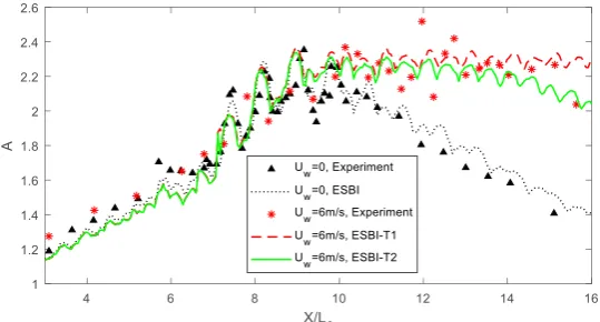
The numerical model is then validated through comparing its predictions with the results obtained in the laboratory by Touboul, et al. [5], in which the focusing wave is generated using the spatial-temporal focusing mechanism and wind velocity is 6 m/s. Simulations by using both ESBI-T1 and ESBI-T2 are performed, where the

𝜂𝜂!" = 0.5. The variation of the amplification factor, 𝐴𝐴(𝑋𝑋) = 𝐻𝐻!"# 𝑋𝑋 /𝐻𝐻!"#, where 𝐻𝐻!"# is the maximum wave

height recorded at location 𝑋𝑋, and 𝐻𝐻!"# is the mean wave height at the probe 1m away from the wave maker,

predicted using the ESBI are presented in Fig. 4, together with the experimental data[5]. It is found that without the wind, the ESBI successfully predicted the variation of 𝐴𝐴(𝑋𝑋) in space and the results agreed very well with experiment data. With the presence of wind, both ESBI-T1 and ESBI-T2 reasonably capture the changes of 𝐴𝐴(𝑋𝑋)

behind the focusing point, although slight differences between the numerical and experimental results were observed. It implies that both ESBI-T1 and ESBI-T2 can give acceptable predictions of the amplification factor and thus can be used for modelling the focusing wave with wind presence.

Figure 4. Comparison of the amplification factor

3.Results and discussion

The validation cases presented in the previous section conclude the results obtained by using the ESBI model are satisfactory, which implies that the ESBI model can deliver reliable results for the purpose of this study. In this section, it is employed to explore the wind effects on rogue waves in spreading seas. The computational domain covers 32×32 peak wave lengths and is resolved into 1024×1024 collocation points, which for example corresponding to a domain size of 23km2 _{considering a typical wave length 150m in the North Sea. A convergent}

test indicates that the current resolution is sufficient to demonstrate the local effects of wind on the rogue waves

modelled by using the focusing wave technique in a short time window, after comparing with the results produced by using further refinement of the mesh (2048×2048) (the error of the maximum surface elevation is about 1.3%). The JONSWAP spectrum with 𝑘𝑘!𝐻𝐻!= 0.3 (𝑘𝑘! the peak wave number) and peak enhancement factor 𝛾𝛾 = 3 are

employed, where the spreading function 𝐺𝐺 𝜃𝜃 = 2/𝜋𝜋 cos! _{𝜃𝜃 is adopted.}

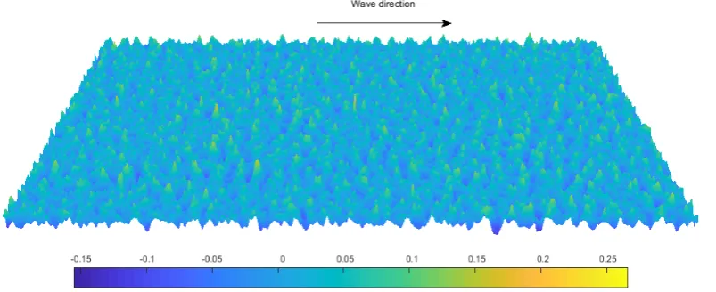
A focusing wave is embedded in the random background waves, by using the method suggested by Wang, et al. [25], where the spectrum is split into three parts, i.e., a transient part, a background part and a correction part. The rogue wave is then embedded by the phase coherence of the transient part, while the spectral shape of the JONSWAP configuration is preserved. Here we only use 1% of the total spectral energy to generate the focusing waves. Since the sheltering mechanism is only effective within a limited time window, the duration of the simulation is made lasting for 20 peak periods, where the focusing occurs at the 10th _{peak period at the centre of the}

computational domain. To have a glance at the spatial scale of the simulation, an illustration of the free surface at the focusing time without presence of wind is shown in Figure 5.

Figure 5. Illustration of the free surface spatial distribution

Three cases with different magnitude of wind speed are considered, i.e., 𝑈𝑈!/𝑐𝑐!= 4, 4.5 and 5, where 𝑐𝑐! is the

wave phase speed corresponding to the peak component, and 𝜂𝜂!"= 0.35. The simulations without the presence of

wind are also performed for comparison, while the cases with wind effects are simulated by using both the ESBI-T1 and ESBI-T2. Note that wave broke in the case 𝑈𝑈!/𝑐𝑐!= 5 by using the ESBI-T2 causing the simulation to

terminate early.

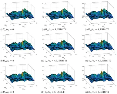
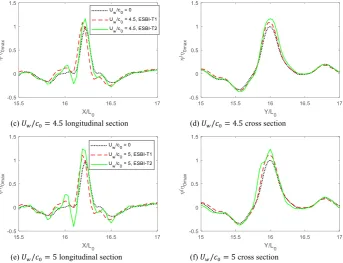
Due to the nonlinearities, the real focusing point and time will be shifted from the specified ones. Therefore, a zoom in look at the free surface spatial distribution at the real focusing time are displayed in Figure 6. A detailed look along the longitudinal and cross sections are displayed in Figure 7.

The results by using both the ESBI-T1 and ESBI-T2 indicate that the maximum crest height of the rogue wave is enlarged due to the wind input as shown in Figure 7(a)(c)(e), as well as the width in cross direction as shown in Figure 7(b)(d)(f). This broadening of the crest is presumably due to the local nonlinear effects [33,34], which is triggered by the local enhancement of waves by the wind. To better examine the magnitude of enlargement, the crest ratio at focusing, i.e., the maximum surface elevation with wind over that without wind, in terms of the wind speed is presented in Figure 8(a), while the energy ratio, i.e., total energy at focusing time against that at initial time, is given in Figure 8(b). It can be found that the crest ratio gradually increases with the increase of the wind speed, as well as the energy ratio, which is understandable as stronger wind can lead to higher drag before breaking occurs and drag is saturated [13].

Jinghua Wang et al. / Procedia IUTAM 26 (2018) 214–226 221 Wang, et al./ Procedia IUTAM 00 (2018) 000–000 7

(a) Without wind presence (b) With wind presence

Figure 3. Free surface spatial distribution. ‘Black line’: ESBI-T1; ‘Red X’: Kharif, et al. [6].

2.2.1 Spatial-temporal focusing wave

The numerical model is then validated through comparing its predictions with the results obtained in the laboratory by Touboul, et al. [5], in which the focusing wave is generated using the spatial-temporal focusing mechanism and wind velocity is 6 m/s. Simulations by using both ESBI-T1 and ESBI-T2 are performed, where the

𝜂𝜂!"= 0.5. The variation of the amplification factor, 𝐴𝐴(𝑋𝑋) = 𝐻𝐻!"# 𝑋𝑋 /𝐻𝐻!"#, where 𝐻𝐻!"# is the maximum wave

height recorded at location 𝑋𝑋, and 𝐻𝐻!"# is the mean wave height at the probe 1m away from the wave maker,

predicted using the ESBI are presented in Fig. 4, together with the experimental data[5]. It is found that without the wind, the ESBI successfully predicted the variation of 𝐴𝐴(𝑋𝑋) in space and the results agreed very well with experiment data. With the presence of wind, both ESBI-T1 and ESBI-T2 reasonably capture the changes of 𝐴𝐴(𝑋𝑋)

behind the focusing point, although slight differences between the numerical and experimental results were observed. It implies that both ESBI-T1 and ESBI-T2 can give acceptable predictions of the amplification factor and thus can be used for modelling the focusing wave with wind presence.

Figure 4. Comparison of the amplification factor

3.Results and discussion

The validation cases presented in the previous section conclude the results obtained by using the ESBI model are satisfactory, which implies that the ESBI model can deliver reliable results for the purpose of this study. In this section, it is employed to explore the wind effects on rogue waves in spreading seas. The computational domain covers 32×32 peak wave lengths and is resolved into 1024×1024 collocation points, which for example corresponding to a domain size of 23km2 _{considering a typical wave length 150m in the North Sea. A convergent}

test indicates that the current resolution is sufficient to demonstrate the local effects of wind on the rogue waves

8 Wang, et al./ Procedia IUTAM 00 (2018) 000–000

modelled by using the focusing wave technique in a short time window, after comparing with the results produced by using further refinement of the mesh (2048×2048) (the error of the maximum surface elevation is about 1.3%). The JONSWAP spectrum with 𝑘𝑘!𝐻𝐻!= 0.3 (𝑘𝑘! the peak wave number) and peak enhancement factor 𝛾𝛾 = 3 are

employed, where the spreading function 𝐺𝐺 𝜃𝜃 = 2/𝜋𝜋 cos! _{𝜃𝜃 is adopted.}

A focusing wave is embedded in the random background waves, by using the method suggested by Wang, et al. [25], where the spectrum is split into three parts, i.e., a transient part, a background part and a correction part. The rogue wave is then embedded by the phase coherence of the transient part, while the spectral shape of the JONSWAP configuration is preserved. Here we only use 1% of the total spectral energy to generate the focusing waves. Since the sheltering mechanism is only effective within a limited time window, the duration of the simulation is made lasting for 20 peak periods, where the focusing occurs at the 10th _{peak period at the centre of the}

computational domain. To have a glance at the spatial scale of the simulation, an illustration of the free surface at the focusing time without presence of wind is shown in Figure 5.

Figure 5. Illustration of the free surface spatial distribution

Three cases with different magnitude of wind speed are considered, i.e., 𝑈𝑈!/𝑐𝑐!= 4, 4.5 and 5, where 𝑐𝑐! is the

wave phase speed corresponding to the peak component, and 𝜂𝜂!" = 0.35. The simulations without the presence of

wind are also performed for comparison, while the cases with wind effects are simulated by using both the ESBI-T1 and ESBI-T2. Note that wave broke in the case 𝑈𝑈!/𝑐𝑐!= 5 by using the ESBI-T2 causing the simulation to

terminate early.

Due to the nonlinearities, the real focusing point and time will be shifted from the specified ones. Therefore, a zoom in look at the free surface spatial distribution at the real focusing time are displayed in Figure 6. A detailed look along the longitudinal and cross sections are displayed in Figure 7.

The results by using both the ESBI-T1 and ESBI-T2 indicate that the maximum crest height of the rogue wave is enlarged due to the wind input as shown in Figure 7(a)(c)(e), as well as the width in cross direction as shown in Figure 7(b)(d)(f). This broadening of the crest is presumably due to the local nonlinear effects [33,34], which is triggered by the local enhancement of waves by the wind. To better examine the magnitude of enlargement, the crest ratio at focusing, i.e., the maximum surface elevation with wind over that without wind, in terms of the wind speed is presented in Figure 8(a), while the energy ratio, i.e., total energy at focusing time against that at initial time, is given in Figure 8(b). It can be found that the crest ratio gradually increases with the increase of the wind speed, as well as the energy ratio, which is understandable as stronger wind can lead to higher drag before breaking occurs and drag is saturated [13].

maximum elevation compared with the CFD simulations where the wind effects are directly modelled, no matter how the critical surface gradient is selected from the range [0.3, 0.4] (see discussionsin Yan & Ma [8]).

(a) 𝑈𝑈!/𝑐𝑐!= 0 (b) 𝑈𝑈!/𝑐𝑐!= 4, ESBI-T1 (c) 𝑈𝑈!/𝑐𝑐!= 4, ESBI-T2

(d) 𝑈𝑈!/𝑐𝑐!= 0 (e) 𝑈𝑈!/𝑐𝑐!= 4.5, ESBI-T1 (f) 𝑈𝑈!/𝑐𝑐!= 4.5, ESBI-T2

(g) 𝑈𝑈!/𝑐𝑐!= 0 (h) 𝑈𝑈!/𝑐𝑐!= 5, ESBI-T1 (i) 𝑈𝑈!/𝑐𝑐!= 5, ESBI-T2

Figure 6. Comparison of the free surface at focusing

(a) 𝑈𝑈!/𝑐𝑐!= 4 longitudinal section (b) 𝑈𝑈!/𝑐𝑐!= 4 cross section

(c) 𝑈𝑈!/𝑐𝑐!= 4.5 longitudinal section (d) 𝑈𝑈!/𝑐𝑐!= 4.5 cross section

(e) 𝑈𝑈!/𝑐𝑐!= 5 longitudinal section (f) 𝑈𝑈!/𝑐𝑐!= 5 cross section

Figure 7. Comparison of the section surface profiles

(a) (b)

Figure 8. Crest ratio (a) and energy ratio (b) at focusing against wind speed

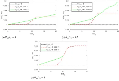
Furthermore, another interesting comparison of the energy ratio evolving in time is shown in Figure 9, from which it can be observed that the total energy in the simulations by using the ESBI-T1 increases suddenly during the focusing stage, and remain constant after de-focusing, while in the ESBI-T2 simulations, the total energy gradually grows over time. This is because the pressure forcing term is not acting on the free surface unless the maximum gradient exceeds the specified value by using the ESBI-T1. However, there is no such assumption and the pressure keeps acting on the free surface during the wave propagation by using the ESBI-T2. In addition, the rate of the energy variation increases significantly when focusing wave occurred in the ESBI-T2 simulations, as can be observed by looking at the slope of the green solid line in Figure 9(b).

Jinghua Wang et al. / Procedia IUTAM 26 (2018) 214–226 223 Wang, et al./ Procedia IUTAM 00 (2018) 000–000 9

maximum elevation compared with the CFD simulations where the wind effects are directly modelled, no matter how the critical surface gradient is selected from the range [0.3, 0.4] (see discussionsin Yan & Ma [8]).

(a) 𝑈𝑈!/𝑐𝑐!= 0 (b) 𝑈𝑈!/𝑐𝑐!= 4, ESBI-T1 (c) 𝑈𝑈!/𝑐𝑐!= 4, ESBI-T2

(d) 𝑈𝑈!/𝑐𝑐!= 0 (e) 𝑈𝑈!/𝑐𝑐!= 4.5, ESBI-T1 (f) 𝑈𝑈!/𝑐𝑐!= 4.5, ESBI-T2

(g) 𝑈𝑈!/𝑐𝑐!= 0 (h) 𝑈𝑈!/𝑐𝑐!= 5, ESBI-T1 (i) 𝑈𝑈!/𝑐𝑐!= 5, ESBI-T2

Figure 6. Comparison of the free surface at focusing

(a) 𝑈𝑈!/𝑐𝑐!= 4 longitudinal section (b) 𝑈𝑈!/𝑐𝑐!= 4 cross section

10 Wang, et al./ Procedia IUTAM 00 (2018) 000–000

(c) 𝑈𝑈!/𝑐𝑐!= 4.5 longitudinal section (d) 𝑈𝑈!/𝑐𝑐!= 4.5 cross section

(e) 𝑈𝑈!/𝑐𝑐!= 5 longitudinal section (f) 𝑈𝑈!/𝑐𝑐!= 5 cross section

Figure 7. Comparison of the section surface profiles

(a) (b)

Figure 8. Crest ratio (a) and energy ratio (b) at focusing against wind speed

Furthermore, another interesting comparison of the energy ratio evolving in time is shown in Figure 9, from which it can be observed that the total energy in the simulations by using the ESBI-T1 increases suddenly during the focusing stage, and remain constant after de-focusing, while in the ESBI-T2 simulations, the total energy gradually grows over time. This is because the pressure forcing term is not acting on the free surface unless the maximum gradient exceeds the specified value by using the ESBI-T1. However, there is no such assumption and the pressure keeps acting on the free surface during the wave propagation by using the ESBI-T2. In addition, the rate of the energy variation increases significantly when focusing wave occurred in the ESBI-T2 simulations, as can be observed by looking at the slope of the green solid line in Figure 9(b).

(a) 𝑈𝑈!/𝑐𝑐!= 4 (b) 𝑈𝑈!/𝑐𝑐!= 4.5

(c) 𝑈𝑈!/𝑐𝑐!=5

Figure 9. Comparison of the energy ratio

Moreover, the real focusing time and location are extracted and examined. It is observed that the focusing time is shifted earlier by the wind in the simulation by using the ESBI-T1, and remain the same despite of the increase of the wind speed. On the contrary, the focusing time is postponed by the wind in the simulations by using the ESBI-T2, where higher wind speed causes further delay. Meanwhile, the focusing location are pushed to the upstream in both the simulations of the ESBI-T1 and ESBI-T2. However, further investigations need to be carried out in order to confirm this observation, as the initially specified focusing time and location can both affect the results as pointed out by Yan & Ma [9].

(a) (b)

Figure 10. Shift of focusing time (a) and location (b) against wind speed

4.Conclusions

In this paper, three-dimensional rogue waves on large scale (32×32 peak wave lengths which is equivalent to 23km2 _{considering a typical wave length 150m in the North Sea) with the presence of wind are simulated in a}

phase-resolved manner by using the Enhanced Spectral Boundary Integral method based on the fully nonlinear potential theory. The wind effects are modelled by using the techniques suggested by Touboul, et al. [5] and Yan & Ma [8]. The results by using both the techniques indicate that higher wind speed produces rogue waves with larger crests

and more energy input. However, the results by using the technique by Touboul, et al. [5] shows a slightly lower maximum crest height and total energy compared with that by using the technique by Yan & Ma [8]. In addition, the focusing time and the location of the rogue waves are also shifted compared with that without the presence of wind. However, only waves with an underlying JONSWAP spectrum are considered, while the range of wind speed is very limited. The conclusion may change if these conditions are different. More tests on a wider range of input parameters will be carried out in the future.

Acknowledgements

The authors gratefully acknowledge the financial support of EPSRC, UK (EP/N006569/1, EP/N008863/1 and EP/M022382/1) and DST-UKIERI project (DST-UKIERI-2016-17-0029).

References

1. C. Kharif, E. Pelinovsky and A. Slunyaev, Rogue Waves in the Ocean, Berlin Heidelberg: Springer-Verlag, 2009.

2. T. A. A. Adcock and P. H. Taylor, The physics of anomalous ('rogue') ocean waves, Reports on Progress in Physics, 2014; 77(10): 105901. 3. N. Mori, P. C. Liu and T. Yasuda, Analysis of freak wave measurements in the Sea of Japan, Ocean Engineering, 2002; 29 (11): 1399-1414. 4. J. P. Giovanangeli, C. Kharif and E. Pelinovski, Experimental study of the wind effect on focusing of transient wave groups, arXiv preprint

physics, 2006; 0607010.

5. J. Touboul, J. P. Giovanangeli, C. Kharif and E. Pelinovsky, Freak waves under the action of wind: experiments and simulations, European Journal Mechanics B/Fluid, 2006; 25: 662-676.

6. C. Kharif, J. P. Giovanangeli, J. Touboul, L. Grare and E. Pelinovsky, Influence of wind on extreme wave events: experimental and numerical approaches, J. Fluid Mech., 2008; 594: 209-247.

7. S. Yan and Q. W. Ma, Numerical simulation of interaction between wind and 2D freak waves, European Journal of Mechanics-B/Fluids, 2010; 29 (1): 18-31.

8. S. Yan and Q. W. Ma, Improved model for air pressure due to wind on 2D freak waves in finite depth, European Journal Mechanics B/Fluid, 2011; 30: 1-11.

9. S. Yan and Q. W. Ma, Numerical study on significance of wind action on 2-D freak waves with different parameters, Journal of Marine Science and Technology, 2012; 20(1): 9-17.

10. K. Iwano, N. Takagaki, R. Kurose and S. Komori, Mass transfer velocity across the breaking air–water interface at extremely high wind speeds, Tellus B: Chemical and Physical Meteorology, 2013; 65 (1): 21341.

11. A. Chabchoub, N. Hoffmann, H. Branger, C. Kharif and N. Akhmediev, Experiments on wind-perturbed rogue wave hydrodynamics using the Peregrine breather model, Physics of Fluids, 2013; 25(10): 101704.

12. N. Takagaki, S. Komori and N. Suzuki, Estimation of friction velocity from the wind-wave spectrum at extremely high wind speeds, IOP Conference Series: Earth and Environmental Science , 2016; 35(1): 012009.

13. N. Takagaki, S. Komori, N. Suzuki, K. Iwano and R. Kurose, Mechanism of drag coefficient saturation at strong wind speeds, Geophysical Research Letters, 2016; 43(18): 9829-9835.

14. A. Toffoli, D. Proment, H. Salman, J. Monbaliu, F. Frascoli, M. Dafilis, E. Stramignoni, R. Forza, M. Manfrin and M. Onorato, Wind generated rogue waves in an annular wave flume, Physical Review Letters, 2017; 118(14): 144503.

15. D. Eeltink, A. Lemoine, H. Branger, O. Kimmoun, C. Kharif, J. Carter, A. Chabchoub, M. Brunetti and J. Kasparian, Spectral up-and downshifting of Akhmediev breathers under wind forcing, Physics of Fluid, 2017; 29(10): 107103.

16. X. Hao and L. Shen, Numerical investigation of energy transfer in coupled wind and wave system, In APS Meeting Abstracts, Portland, Oregon, 2016.

17. T. Li and L. Shen, Numerical study of wind-wave generation at the initial stage, Bulletin of the American Physical Society, Denver, Colorado, 2017.

18. Z. Yang, S. Tang, Y. H. Dong and L. Shen, Numerical study of wind over breaking waves and generation of spume droplets, Bulletin of the American Physical Society, Denver, Colorado, 2017.

19. W. Xiao, Y. Liu, G. Wu and D. K. P. Yue, Rogue wave occurrence and dynamics by direct simulations of nonlinear wave-field evolution, J. Fluid Mech., 2013; 720: 357-392.

20. D. Clamond and J. Grue, A fast method for fully nonlinear water-wave computations, J. Fluid Mech., 2001; 447: 337-355.

21. D. Fructus, D. Clamond, J. Grue and O. Kristiansen, An efficient model for three-dimensional surface wave simulations Part I: Free space problems, Journal of Computational Physics, 2005; 205: 665-685.

Jinghua Wang et al. / Procedia IUTAM 26 (2018) 214–226 225 Wang, et al./ Procedia IUTAM 00 (2018) 000–000 11

(a) 𝑈𝑈!/𝑐𝑐!= 4 (b) 𝑈𝑈!/𝑐𝑐!= 4.5

(c) 𝑈𝑈!/𝑐𝑐!=5

Figure 9. Comparison of the energy ratio

Moreover, the real focusing time and location are extracted and examined. It is observed that the focusing time is shifted earlier by the wind in the simulation by using the ESBI-T1, and remain the same despite of the increase of the wind speed. On the contrary, the focusing time is postponed by the wind in the simulations by using the ESBI-T2, where higher wind speed causes further delay. Meanwhile, the focusing location are pushed to the upstream in both the simulations of the ESBI-T1 and ESBI-T2. However, further investigations need to be carried out in order to confirm this observation, as the initially specified focusing time and location can both affect the results as pointed out by Yan & Ma [9].

(a) (b)

Figure 10. Shift of focusing time (a) and location (b) against wind speed

4.Conclusions

In this paper, three-dimensional rogue waves on large scale (32×32 peak wave lengths which is equivalent to 23km2 _{considering a typical wave length 150m in the North Sea) with the presence of wind are simulated in a}

phase-resolved manner by using the Enhanced Spectral Boundary Integral method based on the fully nonlinear potential theory. The wind effects are modelled by using the techniques suggested by Touboul, et al. [5] and Yan & Ma [8]. The results by using both the techniques indicate that higher wind speed produces rogue waves with larger crests

12 Wang, et al./ Procedia IUTAM 00 (2018) 000–000

and more energy input. However, the results by using the technique by Touboul, et al. [5] shows a slightly lower maximum crest height and total energy compared with that by using the technique by Yan & Ma [8]. In addition, the focusing time and the location of the rogue waves are also shifted compared with that without the presence of wind. However, only waves with an underlying JONSWAP spectrum are considered, while the range of wind speed is very limited. The conclusion may change if these conditions are different. More tests on a wider range of input parameters will be carried out in the future.

Acknowledgements

The authors gratefully acknowledge the financial support of EPSRC, UK (EP/N006569/1, EP/N008863/1 and EP/M022382/1) and DST-UKIERI project (DST-UKIERI-2016-17-0029).

References

1. C. Kharif, E. Pelinovsky and A. Slunyaev, Rogue Waves in the Ocean, Berlin Heidelberg: Springer-Verlag, 2009.

2. T. A. A. Adcock and P. H. Taylor, The physics of anomalous ('rogue') ocean waves, Reports on Progress in Physics, 2014; 77(10): 105901. 3. N. Mori, P. C. Liu and T. Yasuda, Analysis of freak wave measurements in the Sea of Japan, Ocean Engineering, 2002; 29 (11): 1399-1414. 4. J. P. Giovanangeli, C. Kharif and E. Pelinovski, Experimental study of the wind effect on focusing of transient wave groups, arXiv preprint

physics, 2006; 0607010.

5. J. Touboul, J. P. Giovanangeli, C. Kharif and E. Pelinovsky, Freak waves under the action of wind: experiments and simulations, European Journal Mechanics B/Fluid, 2006; 25: 662-676.

6. C. Kharif, J. P. Giovanangeli, J. Touboul, L. Grare and E. Pelinovsky, Influence of wind on extreme wave events: experimental and numerical approaches, J. Fluid Mech., 2008; 594: 209-247.

7. S. Yan and Q. W. Ma, Numerical simulation of interaction between wind and 2D freak waves, European Journal of Mechanics-B/Fluids, 2010; 29 (1): 18-31.

8. S. Yan and Q. W. Ma, Improved model for air pressure due to wind on 2D freak waves in finite depth, European Journal Mechanics B/Fluid, 2011; 30: 1-11.

9. S. Yan and Q. W. Ma, Numerical study on significance of wind action on 2-D freak waves with different parameters, Journal of Marine Science and Technology, 2012; 20(1): 9-17.

10. K. Iwano, N. Takagaki, R. Kurose and S. Komori, Mass transfer velocity across the breaking air–water interface at extremely high wind speeds, Tellus B: Chemical and Physical Meteorology, 2013; 65 (1): 21341.

11. A. Chabchoub, N. Hoffmann, H. Branger, C. Kharif and N. Akhmediev, Experiments on wind-perturbed rogue wave hydrodynamics using the Peregrine breather model, Physics of Fluids, 2013; 25(10): 101704.

12. N. Takagaki, S. Komori and N. Suzuki, Estimation of friction velocity from the wind-wave spectrum at extremely high wind speeds, IOP Conference Series: Earth and Environmental Science , 2016; 35(1): 012009.

13. N. Takagaki, S. Komori, N. Suzuki, K. Iwano and R. Kurose, Mechanism of drag coefficient saturation at strong wind speeds, Geophysical Research Letters, 2016; 43(18): 9829-9835.

14. A. Toffoli, D. Proment, H. Salman, J. Monbaliu, F. Frascoli, M. Dafilis, E. Stramignoni, R. Forza, M. Manfrin and M. Onorato, Wind generated rogue waves in an annular wave flume, Physical Review Letters, 2017; 118(14): 144503.

15. D. Eeltink, A. Lemoine, H. Branger, O. Kimmoun, C. Kharif, J. Carter, A. Chabchoub, M. Brunetti and J. Kasparian, Spectral up-and downshifting of Akhmediev breathers under wind forcing, Physics of Fluid, 2017; 29(10): 107103.

16. X. Hao and L. Shen, Numerical investigation of energy transfer in coupled wind and wave system, In APS Meeting Abstracts, Portland, Oregon, 2016.

17. T. Li and L. Shen, Numerical study of wind-wave generation at the initial stage, Bulletin of the American Physical Society, Denver, Colorado, 2017.

18. Z. Yang, S. Tang, Y. H. Dong and L. Shen, Numerical study of wind over breaking waves and generation of spume droplets, Bulletin of the American Physical Society, Denver, Colorado, 2017.

19. W. Xiao, Y. Liu, G. Wu and D. K. P. Yue, Rogue wave occurrence and dynamics by direct simulations of nonlinear wave-field evolution, J. Fluid Mech., 2013; 720: 357-392.

20. D. Clamond and J. Grue, A fast method for fully nonlinear water-wave computations, J. Fluid Mech., 2001; 447: 337-355.

21. D. Fructus, D. Clamond, J. Grue and O. Kristiansen, An efficient model for three-dimensional surface wave simulations Part I: Free space problems, Journal of Computational Physics, 2005; 205: 665-685.