Fast belief estimation in evidence network models

Fast Belief Estimation in Evidence Network Models

Massimiliano Vasile

Professor, Aerospace Centre of Excellence, Mechanical and Aerospace Engineering University of Strathclyde, James Weir Building, 75 Montrose Street, Glasgow, UK

Email: [email protected]

Gianluca Filippi

Postgraduate Researcher, Aerospace Centre of Excellence, Mechanical and Aerospace Engineering University of Strathclyde, James Weir Building, 75 Montrose Street, Glasgow, UK

Email: [email protected]

Carlos Ortega Absil

PhD candidate, Aerospace Centre of Excellence, Mechanical and Aerospace Engineering University of Strathclyde, James Weir Building, 75 Montrose Street, Glasgow, UK

Email: [email protected]

Annalisa Riccardi

Lecturer, Aerospace Centre of Excellence, Mechanical and Aerospace Engineering University of Strathclyde, James Weir Building, 75 Montrose Street, Glasgow, UK

Email: [email protected]

Summary

This paper introduces a novel approach to model complex engineering systems in the form of a network of interconnected nodes. Each node is associated to a value and an evidence measure associated to that value. The Belief and Plausibility associated to the total value of the network is then estimated with a fast decomposition technique that allows for several order of magnitude reduction in computational time under some assumptions on the properties of the network. The modeling approach and associated Belief estimation technique are proposed for the optimisation of complex engineering systems under epistemic uncertainty. The methodology is applied to the preliminary design of a small satellite where some quantities are affected by an epistemic uncertainty. In addition, the paper describes a surrogate method that provides a faster evaluation of the belief curve.

Keywords:Evidence, Belief, Decomposition, Optimization.

1 Introduction

The quantification of uncertainty in complex engineering systems is computationally challenging. Part of the challenge comes from the computational cost of propagating uncertainty through the system model. This cost is typically exponential with problem dimension and can become quickly untreatable even for systems of moderate size. Uncertainty can be modeled as a random process with an associated probability distribution. In a number of cases, however, the knowledge on the probability distribution is missing or is uncertainty in itself. In this later case the uncertainty is epistemic as there is a fundamental lack of knowledge or information.

The paper proposes to model a complex engineering system as a particular network of interconnected

components. Each component is exchanging information with other components through a set of exchange variables. The quantity associated to each component and the exchange variables are assumed to be affected by uncertainty, where this uncertainty can be epistemic in nature. In particular, we propose the use of Dampster-Shafer theory of evidence to model epistemic uncertainty.Shafer(1976a) _{For this reason the network model} representing the engineering system is here called Evidence Network Model (ENM). Evidence theory, that belongs to a class of mathematical theories known as Imprecise Probabilities, can be seen as an extension to standard probability theory and is devised to properly handle the imprecision that comes with epistemic uncertainty.

characterised by a global quantity of interestF:

F:D×U⊆Rm+n→R (1)

whereF depends on some uncertain parametersu∈U⊂

Rm and design parametersd∈D⊂Rn. The setDis the available design space andU the uncertain space. One or more intervals are defined for each uncertain variable ui

and for each one of those intervals a level of confidence on the values of u (bpa, basic probability assignment) is assigned. All the Cartesian products of the uncertain intervals with a non-zero basic probability assignment are called Focal Elements (FE). Assuming strong independence among uncertain variables the bpa associated to each FE is the product of the bpas associated to each interval. For a given design d, we can then calculate two cumulative quantities, Belief (Bel) and Plausibility (Pl),Shafer(1976b)that provide the lower and upper belief in the occurrence of a particular event or the truth of a proposition on the value of the network.

Once the ENM is defined, a decomposition technique is used to quickly quantify the uncertainty associated to

F. The decomposition approach, proposed in this paper, starts from some suitable assumptions on the nature of the exchange variables and the dependency of the quantity of interest F on these variables. It then proceeds by decomposing the ENM and incrementally reconstructing Belief and Plausibility at a computational cost that is orders of magnitude lower than a full computation of Belief and Plausibility.Alicino and Vasile(2014a)

The paper presents some illustrative examples: three synthetic function and one real problem, the design of a small satellite in which three subsystems are affected by epistemic uncertainty.

2 Evidence Network Models

A generic complex system can be represented as a network, where each node represents one of its subsystem and links represents sharing of information between subsystems. We can then define a functionFas

F(d,u) =

N

∑

i=1

gi(d,ui,hi(d,ui,ui j))

whereNis the number of subsystems involved,hi(d,ui,ui j)

is the vector of scalar functionshi j(d,ui,ui j)where j∈Ji

andJi is the set of indexes of nodes connected to thei-th

node; ui are the uncertain variables of subsystem i not

shared with any other subsystems andu_{i j}are the uncertain variables shared among subsystems i and j. Please note that accordingly to our notationui j=ujiand the functions gi(·,·,·) represent quantities computing by the governing

equations of the different subsystems. In a fully connected

network as in Figure 1 the functionFis:

F(d,u) = g1(d,u1,h12(d,u1,u12),h13(d,u1,u13)))+

g2(d,u2,h21(d,u2,u12),h23(d,u2,u23)))+

g3(d,u3,h31(d,u3,u13),h32(d,u3,u23)).

(2) We then callui,uncoupledvariables because they influence

u12

u23

u13 g1(d,u1,u12,u13)

g2(d,u2,u12,u23) g3(d,u3,u13,u23)

Figure 1: Evidence Network Model of a generic systemF

composed of three sub-systems with coupled variablesu12, u13andu23.

only one subsystem andui jcoupledvariables because they

influence two subsystems. Hence for the example in Figure 1 the uncertain vector can be ordered as

u= [u1,u2,u3,u12,u13,u23]T.

In the following we will study only the case in which the functionsgi(·,·,·)are always positive semidefinite and are

monotonic with respect to each functionhik.

Given a design, or decision, value ˜d∈ D we will call

worst case scenario the vector u that corresponds to the maximum ofFover the spaceU:

u=argmax

u∈U

F(ed,u) (3)

likewise we can callbest case scenariothe quantity: ¯

u=argmin

u∈U

F(ed,u) (4)

We can now define an event in the space U, or a proposition on the value ofF, as the setAsuch that:

From this definition it is clear that for every designd∈D

the worst case scenario corresponds to A =U, because

ν=maxu∈UF(d,u), and analogously the best case scenario

has zero measure. Each uncoupled uncertain vectorui is

defined over a set of boxes named Θi=∪kθk,i and each

coupled uncertain vectorui jis defined over the set of boxes

Θi j=∪kθk,i j. We define the set

Θ=[

i

θi= (×m_i=u1Θi)×(×

mc

i,j=1Θi j)

where mu is the number of uncoupled uncertain vectors

(equal to the number of subsystems) andmcis the number

of coupled uncertain vectors. and the hyperpower set

DΘ_{= (}

Θ,∪,∩) (6)

as the set composed of the elements ofΘ, their union and intersection. In the following the spaceU :=DΘ_{. We} can then define quantities associated to the belief in the occurrence of the eventA:

Bel(A) =

_∑

θ⊂A,θ∈U

bpa(θ) (7)

Pl(A) =

_∑

θ∩A6=0,θ∈U

bpa(θ) (8)

where bpa(θ) is the basic probability assignment

associated to θ, an element of the power set. It is

important to note that if the hi j functions were known

with certainty the nodes composing the network would be decoupled and statistically independent. We also note that in order to identify if aθ is fully included inAwe need to find the maximum ofF with respect tou∈θ. Likewise an intersection with A requires computing the minimum ofFwith respect tou∈θ. Given that the subsetsθ, their unions and intersections come from a cross product, it is clear that the number of maximisation and minimisation increases exponentially with the number of dimensions. The computation of the Belief in the occurrence ofA is, therefore, an exponentially complex operation. In the following section a technique is proposed to compute an approximation to (7) by exploiting some of the properties of the ENM listed above. In particular we will exploit the following three properties:

1. The contribution of the coupled varaible ui j to the

valueFmanifests through the scalar functionshi jand hji.

2. Allgifunctions are positive semidefined.

3. All gi functions are monotonically increasing with

respect tohi jfor every j.

3 Decomposition Algorithm

In order to reduce the computational complexity of the calculation of Bel(A) we propose a decomposition

technique that exploits the three properties defined in the previous section. The decomposition algorithm aims at decoupling the sub-systems over the uncertain variables in order to optimise only over a small sub-set of the Focal Elements (Algorithm 1); this procedure requires the following steps:

1. Solution of the optimal worst case scenario problem: min

d∈Dmaxu∈UF(d,u) (9)

2. Maximisation over the coupled variables and computation ofBel(A).

3. Maximisation over the uncoupled variables. 4. Reconstruction of the approximationBelf(A).

Point 1 will not be discussed in this paper. An algorithm can be found in,Vasile(2014)Alicino and Vasile(2014b) and more recently in.Ortega and Vasile(2017) _{The result of the solution of} problem (9) are the values ˜dandu, thus, in the following the assumption is that ˜dis already available.

3.1 Maximisation over the coupled variables and evaluation of the partial Belief curves

For each coupled vectorui ja maximisation is run over each

Focal Elementθk,i j⊆Θi j⊆U, givenedand keeping fixed all the other components ofu. Taking again the example in Figure 1 we have:

ˆuk,12= argmax

u12∈θk,12

F(ed,u₁,u₂,u₃,u12,u13,u23),∀θk,12⊂Θ12

ˆuk,13= argmax

u13∈θk,13

F(ed,u₁,u₂,u₃,u₁₂,u13,u23),∀θk,13⊂Θ13

ˆuk,23= argmax

u23∈θk,23

F(ed,u₁,u₂,u₃,u₁₂,u₁₃,u23),∀θk,23⊂Θ23

(10) For easiness in the notation we will indicate with

F(ui j):=F(d˜,u1, ...,ui j, ...,ui+1j, ...).

We can then compute the partial belief associated only to the coupled variables with indexi j:

Bel(F(ui j)<ν) =

∑

θk,i j|maxu_{i j}∈θ_{k,i j}F(ui j)≤ν

bpa(θk,i j) (11)

The calculation of the partial belief can be found in Algorithm 1, line 6. Once the partial belief curve, for each coupled vector, is available, one can sample these curves, by taking a succession of{ν1, ...,νNS=ν}values, and find the corresponding values of the coupled vectors_buq_{k,i j}. These values will be used in the next step to decouple the functions

gi(gj) and compute the maxima of eachgi(gj) with respect

3.2 Optimization over the uncoupled vectors

For each levelq, given a fix value of the coupling functions, one can study eachgiindependently of the others. The idea

is to run an optimisation for each functiongiover only the

uncoupled vectorui. With the example in Figure 1 in mind,

having

ˆ

h_{i j}q(ui):=hi j(d˜,ui,uˆq_{i j})

where ˆuq_{i j}:=uˆq_k∗_{,i j} :k∗=argmax_kF(uˆq_{k,i j}), is one of the

maxima of the maxima attained by the coupled variableui j.

For every Focal Elementθk,i∈Θiwe have:

ˆuq_k,1=argmax

u1∈θk,1

g1(ed,u1,bhq₁₂(u1),bhq₁₃(u1)),∀θk,1⊂Θ1

ˆuq_k,2=argmax

u2∈θk,2

g2(ed,u2,bh

q

21(u2),bh

q

23(u2)),∀θk,2⊂Θ2

ˆuq_k,3=argmax

u3∈θk,3

g3(ed,u3,bhq₃₁(u₃),bhq₃₂(u₃)),∀θ_k,3⊂Θ₃

(12) with the corresponding values ˆgq_k,1, ˆg_kq_,2and ˆgq_k,3.

3.3 Complexity Analysis

From the definition of the hyperpower set in (6) it is clear that the number of focal elements increases exponentially with the number of dimensions. Even if one limits theU

space to the soleΘthe total number of Focal Elements (FE)

for a problem withmuncertain variables, each defined over

Nkintervals, is:

NFE= m

∏

k=1

Nk. (13)

In terms of coupled and uncoupled uncertain vectors we can write:

NFE = mu

∏

i=1

pu i

∏

k=1 N_iu_,k

! _m

c

∏

i=1

pc i

∏

k=1 N_ic_,k

!

. (14)

wherepu_i and pc_i are the number of components of the i− thuncoupled and coupled vector, respectively, andN_iu_,kand

N_ic_,kare the number of intervals of thek−thcomponents of thei−thuncoupled and coupled vector respectively. The total number of focal elements that needs to be explored in the decomposition is instead:

N_FEDec=Ns mu

∑

i=1 N_FEu _,i+

mc

∑

i=1

N_FEc _,i (15)

considering the vector of uncertainties ordered as u= [u1, ...,umu

| {z }

uncoupled

,u1, ...,umc

| {z }

coupled ]

where andNsis the number of samples in the partial belief

curves, N_FEc _,i =∏p

c i

k=1Nic,k and NFEu ,i =∏ pu

i

k=1Niu,k. This

means that the computational complexity to calculate the

maxima of the function F within the focal elements is polynomial with the number of subsystems and remains exponential for each individual uncoupled or coupled vector.

3.4 Reconstruction

Once all the maxima over the focal elements of the uncoupled variables are available for each sample q one can calculate an approximation of Bel(F(d,u) <ν) as follows. From Eq. (12), for each sampleq the maximum associated to focal elementθk =θk1,1×θk2,2×θk3,3, for k=1, ...N_FE,1·NFE,2·NFE,3, given the condition of positive semidefinition ofgi, is:

max (u1,u2,u3)∈θk

F(d˜,u1,u2,u3,uˆq12,uˆ

q

13,uˆ

q

23) =gˆ

q k1,1+gˆ

q k2,2+gˆ

q k3,3

(16) with associated basic probability assignment:

bpaq(θk) =bpa(θk1,1)bpa(θk2,2)bpa(θk3,3)∆Bel q ₍₁₇₎

where∆Belq=∏i j∆Belqi jare the contributions of the partial

belief curves in (11). In other words, thebpaof eachθkis

the product of all thebpa’s of the FE of each uncoupled variable scaled with the product of the belief values of the samples drawn from the partial belief curves(Line 18). The approximation of the belief is then computed as:

f

Bel(F(d,u)≤ν) =

_∑

∑

bpaq(θk) (18)

If the decomposition drastically reduces the number of maximisations, the reconstruction still requires an exponential number of multiplications of bpa’s. Thus, the computational cost of the reconstruction step would increase exponentially with the number of sub-systems if the full curve was required. In this case the number of times that (17) has to be evaluated would be:

Nevals=Ns mu

∏

i=1

N_FEu _,i (19)

If the decomposition is used to evaluateBel(F(d,u)< ν), for a given dand a single threshold ν, then a partial belief curve could be reconstructed only in a neighborhood ofνat a reduced computational cost.

For a given sampleq, consider the vector ˆgq_i = [gˆq_i,1, ...,gˆq_i,Nu

FE,i]

T

of all the maxima of a functiongiover all the focal elements θk,iand the collection of vectors

Γ= [γqik] _{q =1, ...,N} S i =1, ...,mu k =1, ...,N_FEu _,i

organised as in Table 1. The approximated belief curve in Eq. (18) can be computed by taking the sum of the bpa’s for every row ofΓand then adding up all the rows.

Now, givenν one can filter out all the components ˆgq_k,i

of each vectorˆgq_i that satisfies the relationship:

ˆ

gq_k,i+

NU

∑

i=1 min

k ˆg q

i >ν (20)

If condition (20) is applied to every vector in Γ we obtain a new collection ΓL. Symmetrically we can also

construct the collectionΓRby filtering the vectors inΓwith

the following condition:

ˆ

gq_k,i+

NU

∑

i=1 max

k ˆg q

i <ν (21)

The computation of Bel(F(d,u)≤ν) is now realised by

taking from each row of the two collections ΓL and ΓR

the ones that contain the least amount of focal elements, i.e. the ˆgq_i vectors with the lowest number of components, and form the new collectionΓν. We can now calculate the

approximated belief as in Eq.(18) but using the rows and columns of matrixΓν.

Table 1: information used in the reconstruction step

sub1 sub2 ... subi ... submu

sample1 ˆg11 ˆg12 ... ˆg1i ... ˆg1mu sample2 ˆg21 ˆg22 ... ˆg2i ... ˆg2mu

... ... ... ... ... ... ...

sampleq ˆgq1 ˆg

q

2 ... ˆg

q

i ... ˆg q mu

... ... ... ... ... ... ...

sampleNs ˆg

Ns

1 ˆg

Ns

2 ... ˆg

Ns

i ... ˆg Ns

mu

The new computational cost of the reconstruction after filtering is:

Nevals=

Ns

∑

q=1

mu

∏

i=1

dim(ˆgq_i), ˆgq_i ∈Γν (22)

Figure 2 shows an example of reconstruction, after decomposition, in a neighborhood ofν=300. The black curve in Figure 2 is the exact belief curve computed for problem in test case 1 in the results section. In this case, the reconstruction without filtering (red curve in Figure 2 ) requiresNevals=2(9×9) =162, while the reconstruction after filtering (blue curve in Figure 2 ) requiresNevals=90. 4 Theoretical Considerations

In this section we prove that the decomposition, as explained in the previous sections, always produces an approximated belief that is lower or equal to the exact one. Suppose that a function F has the following form (for easiness of notation we omit the design variabled that is fixed during the decomposition and we assume only two

0 50 100 150 200 250 300 350 400 450 0

0.1 0.2 0.3 0.4 0.5 0.6 0.7 0.8 0.9 1

objective function

Belief

Exact Curve

Decomposition with partial reconstruction Decomposition with total reconstruction

Figure 2: Reconstruction of the Belief curve in the neighborhood of the threshold ν = 300. The objective

function is Test case 1 withu∈ {[−5,−1]∪[−3,0]∪[1,2]}6 andbpa= [0.3,0.3,0.4]6; the curve has been reconstructed with two samples in different positions compared with Figure 3.

uncoupled vector and one coupled vector):

F(u1,u2,u12) =g1(u1,h12(u1,u12)) +g2(u2,h21(u2,u12)) (23) withu1∈Θ1,u2∈Θ2,u12∈Θ12andΘ=Θ1×Θ2×Θ12; and the functionsg1(·,·)andg2(·,·)are positive definite i.e. g1(u1,h12(u1,u12)) ≥0, (24) g2(u2,h21(u2,u12)) ≥0 ∀(u1,u2,u12)∈Θ If we introduce the spacesΩ12⊆Θ12andΩ=Θ1×Θ2×

Ω12⊆Θwe can define the maximiser of functionF inΩ

as:

(u₁,u₂,ˆu12) =argmax

u12∈Ω12

F(u₁,u₂,u12) (25) whereu₁andu₂are the uncoupled components of vectoru solution of problem (3). We can now prove the following lemmas.

Lemma 4.1. Given a function F as in (23) if the following monotonicity conditions hold true: givenu1₁₂andu2₁₂inΩ12

g1(u1,h12(u1,u112)) ≤ g1(u1,h12(u1,u212)) l

h12(u1,u112) ≤ h12(u1,u212) and

g2(u2,h21(u2,u1₁₂)) ≤ g2(u2,h21(u2,u2₁₂)) l

h21(u2,u112) ≤ h21(u2,u212)

(26)

for allu1∈Θ1andu2∈Θ2. Then

F(u1,u2,u12)≤maxu1∈Θ1g1(u1,h12(u1,ˆu12))

+maxu2∈Θ2g2(u2,h21(u2,ˆu12))

(27)

Algorithm 1Decomposition 1: Initialise

2: Uncoupled vectorsuu= [u1,u2, ...,ui, ...,umu] 3: Coupled vectorsuc= [u12,u13, ...,ui j, ...,umc] 4: fora given designed do

5: Compute (ed,u_u,u_c) = (argmaxF(ed,u_u,uc)

6: forallui j∈ucdo

7: forall Focal Elementsθk,i j⊆Θi jdo

8: Fbk,i j=maxui j∈θk,i jF(ed,uu,ui j) 9: _bu_k,i j=argmaxui j∈θk,i jF 10: Evaluatebpa(θk,i j)

11: Evaluate partial Belief curveBel(F(ui j)≤ν) 12: end for

13: fornumber of samplesdo 14: Evaluate∆Belq,_buk,i jandFbk,i j

15: end for 16: end for

17: forall the combinations of samplesdo 18: forallu_i∈u_udo

19: forall Focal Elementsθk,i⊆Θido

20: Run

Fmax,k,i=maxθk,iF(ed,buc,ui) 21: Evaluatebpa(θk,i)

22: end for 23: end for

24: forall the combinations of Focal Elements

θt∈Θ1×Θ2×...×Θmu do 25: EvaluateFmax,k≤ν 26: Evaluatebpak

27: end for

28: Evaluate the Belief for this sample by constructing collectionΓν

29: end for

30: Add up all belief values for all samples 31: end for

Proof. Given monotonicity condition (26) and the fact that functionsg1(·,·)andg2(·,·)are positive semidefined, we have:

F(u1,u2,u12) =g1(u1,h12(u1,u12)) +g2(u2,h21(u2,u12)) ≤g1(u1,h12(u1,ˆu12)) +g2(u2,h21(u2,ˆu12)) ≤maxu1∈Θ1g1(u1,h12(u1,ˆu12))+

+maxu2∈Θ2g2(u2,h21(u2,ˆu12))

(28) for all(u1,u2,u12)∈Ω.

Lemma 4.2. Given a function F as in (23), if monotonicity condition (26) holds true then there is at least one ˆu12∈

θ12⊂Ω12such that:

max (u1,u2,u12)∈Ω

F(u₁,u₂,u₁₂) = max

u1∈Θ1

g1(u1,h12(u1,ˆu12))+

+max

u2∈Θ2

g2(u2,h21(u2,ˆu12)) (29)

Proof. From Lemma 4.1, since the inequality holds

∀(u1,u2,u12)∈Ωit holds also for the value that attains the

maximum: max (u1,u2,u12)∈Ω

F(u1,u2,u12)≤ max

u1∈Θ1

g1(u1,h12(u1,ˆu12))+

+ max

u2∈Θ2

g2(u2,h21(u2,ˆu12))

(30) Let us assume now that the solution (u∗₁,u∗₂,u∗₁₂) := argmax_(u

1,u2,u12)∈ΩF(u1,u2,u12)is such that: F(u∗₁,u∗₂,u∗₁₂)< max

u1∈Θ1

g1(u1,h12(u1,ˆu12))+

max

u2∈Θ2

g2(u2,h21(u2,ˆu12)) (31) In this case solution(u∗₁,u∗₂,u∗₁₂)is not a global maximiser. As a consequence if solution (u∗₁,u∗₂,u∗₁₂) is a global maximum ofFthen it must be that:

max (u1,u2,u12)∈Ω

F(u1,u2,u12) = max

u1∈Θ1

g1(u1,h12(u1,ˆu12))+

+max

u2∈Θ2

g2(u2,h21(u2,ˆu12))

(32)

Lemma 4.1 and 4.2 allow us to demonstrate the following fundamental theorem on the accuracy of the decomposition.

Theorem 4.3. If the decomposition is applied to calculate an approximation Belf(F(u)<ν) of Bel(F(u)<ν) and monotonicity condition (26) holds true, then:

f

Bel(F(u1,u2,ˆu12)≤ν)≤Bel(F(u1,u2,u12)≤ν) (33) foru1∈Θ1,u2∈Θ2,u12∈Ω12,ˆu12∈Ωˆ12andΩ12⊂Ωˆ12. Furthermore,

f

Bel(F(u1,u2,ˆu12)≤ν) =Bel(F(u1,u2,u12)≤ν) (34) whenΩ12=Ωˆ12.

Proof. For a givenνconsider the corresponding set of focal

elements

Ων=

[

t

{θt: max u1,u2,u12∈θt

F(u1,u2,u12)<ν} (35)

where for everytit exists a set of indexes{i,j,k}such that

then the exact cumulative belief function is:

Bel(F(u1,u2,u12)≤ν) =

_∑

bpa(θ1,i)bpa(θ2,j)bpa(θ12,k)

(37) Consider now the approximated cumulative belief function

f

Belq(F(u₁,u₂,u₁₂)≤ν)constructed as follows: f

Belq(F(u1,u2,u12)≤ν) =

_∑

∑

bpa(θ1i)bpa(θ2,j)Belq(Ω12)

(38) for allθ1,i∈Θ1andθ2,j∈Θ2such that:

maxu1∈θ1,ig1(u1,ˆu

q

12) +maxu2∈θ2,jg2(,u2,ˆu

q

12)<ν (39) with

ˆuq₁₂=argmax

u12∈Ωq₁₂

F(u₁,u₂,u12) (40) Note that for a single sample q the ∆Belq in (17) is

computed from Bel=0, therefore, ∆Belq=Belq. From

Lemma 4.1 we can say that:

max_(u1,u2,u12)∈θtF(u1,u2,u12)< maxu1∈θ1,ig1(u1,ˆu

q

12) +maxu2∈θ2,jg2(u2,ˆu

q

12) ∀q|Ων⊂Ωq

(41)

which means that by construction f

Belq(F(u1,u2,u12)≤ν)≤Bel(F(u1,u2,u12)≤ν).

From Lemma 4.2 we know that forΩν=Ωq:

max_(u

1,u2,u12)∈ΩνF(u1,u2,u12) =

maxu1∈Θ1g1(u1,ˆu q

12) +maxu2∈Θ2g2(u2,ˆu q

12)

(42) Therefore, comparing Eq.(38) with Eq.(37) we can say that

f

Belq(F(u1,u2,u12)≤ν) =Bel(F(u1,u2,u12)≤ν).

Eq. (41) suggests a possible definition of monotonicity for multivariate functions. LetP(Θ) be the set of all the

subsets ofΘ. IfΩ1andΩ2are two elements ofP(Θ)we say

thatFis monotonically increasing with respect tou∈P(Θ)

if:

max

u∈Ω1

F(u)≤max

u∈Ω2

F(u)⇔Ω1⊆Ω2 (43) 5 Surrogate Approach

The decomposition drastically reduces the number of optimisations required to calculate the cumulative belief function. However, the number of focal elements for each coupled or uncoupled vector can be considerable. Thus, in this paper we propose the use of a surrogate of the space of the maxima over the indexes of the focal elements to further reduce the number of maximisations required to compute the belief curve.

To be more specific, if ji is the index identifying

the j−th interval along dimension i, assuming that all intervals are adjacent and the frame of discernment is

limited to Θ, the idea is to construct an approximation to the functionF∗(j1, ...,ji, ...,jm):N→Rsuch that, for each focal elementθkdefined by the product of a particular

combination of intervals identified by the vector of indexes J_k= [j1,j2, ...ji, ...jm]T_k, the valueF∗(Jk)is the maximum

ofF(u)withu∈θk.

Given ed ∈ D, we will use a Kriging modelTardioli et al(2015)Tardioli, Kubicek, Vasile, Minisci, and Riccardi to interpolate some of the maxima F∗ evaluated for a limited set index vectors Jk, and to predict the value of

the maxima at other locations (other combinations of intervals). Once an estimation of the belief is computed with the surrogate model a further refinement can be obtained via decomposition or full belief calculation.

The surrogate of the functionF∗ could be constructed also over theU space. However, in this case, in order to sample the surrogate one would need to generate sample vectorsuin such a way that each vector falls in only one focal element. Thus, one would need, anyway, to first take a sample of indexes and then generate auvector within the focal element corresponding to the sampled index set.

Note that in this specific case, as the number of intervals per dimension tends to infinity, the number of focal elements also tends to infinity and the distribution of bpa’s approaches a continues density function.

6 Robust Design Trade-off Curve

Once the cumulative belief value is computable for each designdand eachν, one can maximise the belief associated toν by selecting an optimald. This can be formulated as the following bi-objective problem:

minν

max_dBel(F<ν) (44)

The value of ν for which Bel is maximal, can be obtained by solving a deterministic global min-max problem:

νmax=min

d maxu F(d,u) (45)

Likewise the best value of ν for which Pl = 0 can be obtained by solving the deterministic global min-min problem:

νmin=min

d minu F(d,u) (46)

Once the min-max and min-min values are available one can use the decomposition technique to estimate Bel for every ν ∈[νmin,νmax] and optimise the whole Bel curve

following Algorithm 2. Note that the result is a set of d values in which each d provides the maximum belief only for a given ν. This means that the belief curve

corresponding to thedassociated to a particularν can be suboptimal for otherν’s.

7 Results

Algorithm 2Robust Trade-off Curve 1: Initialisation

2: Computeνmin=min min andνmax=min max

3: foreachν∈[νmin,νmax]do

4: Compute maxdBelf(F≤ν) 5: end for

problem. The first four cases are testing the decomposition algorithm and its ability to deliver a good approximation to the true belief curve at a fraction of the computational cost. The fifth case will test the use of the surrogate model and the optimisation of the belief curve for differentν’s.

7.1 Decomposition Test Set

In test cases 1 and 2 each partial belief curves was sampled the same number of timesNs=costmc.

On the contrary, in test cases 3 and 4, different partial Belief curves were sampled differently so that the number of samples is:

Ns= mc

∏

i=1 Ns,i

Table 2 reports the number of intervals per dimension, in the uncertainty space, the range of thedvector and the bpa’s associated to each interval, for cases 1,2 and 3. Case 1 in particular was solved for an increasing number of intervals per dimension. In all tests, the uncertainty space isU=Θ

and uncertain variables are uncorrelated.

Table 2: Design, uncertain parameters and bpa structure for test cases 1, 2 and 3.

# Parameters

1

d∈[−5,5]2

u∈ {[−5,−1],[−3,0],[1,2]}6 u∈ {[−5,−1],[−3,0],[1,2],[3,5]}6 u∈ {[−5,−1],[−3,0],[1,2],[2.5,4],[3,5]}6

u∈ {[−5,−1],[−3,0],[1,2],[2.1,3],[3.1,4.5],[4,5]}6 u∈ {[−5,−1],[−3,0],[1,2],[2.1,3],

[3.1,4.5],[4,5],[3,7]}6

2

d∈[0,3]13

u∈ {[−5,−4],[−3,0],[−1,3]}13 bpa =[0.1,0.25,0.65]13

3

d∈[0,3]8

u∈ {[−5,−4],[−3,0],[−1,3]}8 bpa =[0.1,0.25,0.65]8

7.1.1 Decomposition: test case 1

In test case 1, the cost function F is composed of two sub-functionsg1andg2:

  

 

F=g1+g2

g1=10u21+|u2|u25+

u4 6

100+d1|d2| g2=|u3|+u24

|u5|

10 +u26+|d1|

The uncertain vectoruis: 

   

   

u= (u₁,u₂,u₁₂)

dim(u1) =2 u1= (u1,u2) dim(u₂) =2 u₂= (u3,u4) dim(u12) =2 u12= (u5,u6)

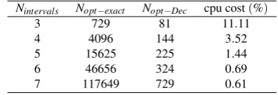
whereu12 is the vector of coupled variables and u1 and u2are the vectors of uncoupled variables. Different belief curves were computed for an increasing number of intervals per dimension. Tab 3 shows the computational cost of the decomposition compared to an exact calculation of the curve. The first column is the number of intervals per dimension, the second column the number of maximisation required for an exact calculation of the belief, while the third column is the number of maximisation used in the decomposition. The last column is the computational time of the decomposition with respect to the exact calculation. The gain in computational time increases as the number of intervals increases.

Tab 4 and Fig 3 show, for a fixed number of interval u∈ {[−5,−1]∪[−3,0]∪[1,2]}6_{, the convergence of the} curve computed with the decomposition for an increasing number of samples. The last column in Tab 4 is the relative computational cost. To be noted that for 6 samples the approximated curve is almost identical to the exact one but the computational cost is only 16%.

Table 3: Test case 1; results with 4 samples in the partial Belief curve.

Nintervals Nopt−exact Nopt−Dec cpu cost(%)

3 729 81 11.11

4 4096 144 3.52

5 15625 225 1.44

6 46656 324 0.69

7 117649 729 0.61

Table 4: Test case 1; results with 3 intervals for each dimension ofuand different number of samples.

N_samplespartial N_samplestotal Nopt−exact Nopt−Dec cpu cost(%)

1 1 729 27 3.7

2 2 729 45 6.17

3 3 729 63 8.64

4 4 729 81 11.11

5 5 729 99 13.58

6 6 729 117 16.05

7.1.2 Decomposition: test case 2

0 50 100 150 200 250 300 350 400 450 objective function 0 0.1 0.2 0.3 0.4 0.5 0.6 0.7 0.8 0.9 1 Belief exact Belief 1 sample 2 samples 3 samples 4 samples 5 samples 6 samples

Figure 3: Test case 1, convergence withu∈ {[−5,−1]∪

[−3,0]∪[1,2]}6_{andbpa= [0.3,0.3,0.4]}6

                          

F=g1+g2+g3+g4

g1= 2

∑

i=1

(di−ui)2+1₂

9

∑

i=6

(di−ui)2

g2= (d3−u3)2+1₂ 7

∑

i=6

(di−ui)2+1₂

11

∑

i=10

(di−ui)2

g3= (d4−u4)2+(d8−u8) 2

2 +

(d10−u10)2

2 +

1 2

13

∑

i=12

(di−ui)2

g4= (d5−u5)2+₂1(d9−u9)2+1₂ 13

∑

i=11

(di−ui)2

where the uncertain vectoruis composed of four uncoupled vectors:u1,u2,u3andu4, and six coupled vectors,u12,u13, u14,u23,u24andu34. The results are shown in Fig 4 and Tab 5 In this case only 3 samples are sufficient to achieve almost the exact value of the belief, though with a computational cost of 0.82% of the exact one.

                                              

u= (u₁,u₂,u₃,u₄,

u12,u13,u14,u23,u24,u34)

dim(u₁) =2 u1= (u1,u2)

dim(u2) =1 u2= (u3)

dim(u₃) =1 u3= (u4)

dim(u4) =1 u4= (u5)

dim(u12) =2 u12= (u6,u7)

dim(u13) =1 u13= (u8)

dim(u14) =1 u14= (u9)

dim(u23) =1 u23= (u10)

dim(u24) =1 u24= (u11)

dim(u34) =2 u34= (u12,u13)

1.8 1.85 1.9 1.95 2 2.05 2.1 2.15 2.2

objective function _×104

0 0.2 0.4 0.6 0.8 1 1.2 Belief exact Belief 1 sample 2 samples 3 samples

Figure 4: Test case 2, convergence with bpa = [0.1,0.25,0.65]13

Table 5: Test case 2 with different number of samplings.

N_samplespartial N_samplestotal Nopt−exact Nopt−Dec cpu cost(%)

1 1 1594323 48 3e−3

2 64 1594323 1182 7.4e−2

3 729 1594323 13152 0.82

4 4096 1594323 73758 4.6

7.1.3 Decomposition: test case 3

The functionFis here composed of three sub-functions:

                  

F=g1+g2+g3

g1= (d1−u1)2+1₂ 7

∑

i=4

(di−ui)2

g2= (d2−u2)2+12 5

∑

i=4

(di−ui)2+12(d8−u8)2

g3= (d3−u3)2+1₂ 8

∑

i=6

(di−ui)2

0 50 100 150 200 250 300

objective function

0 0.1 0.2 0.3 0.4 0.5 0.6 0.7 0.8 0.9 1

Belief

exact Belief 1 sample 2 samples 4 samples 8 samples 30 samples 108 samples 243 samples

Figure 5: Test case 3, convergence with bpa = [0.1,0.25,0.65]8

the partial curves. 

          

          

u= (u1,u2,u3,u12,u13,u23)

dim(u1) =1 u1= (u1)

dim(u2) =1 u2= (u2)

dim(u3) =1 u3= (u3)

dim(u12) =2 u12= (u4,u5) dim(u13) =2 u13= (u6,u7) dim(u23) =1 u23= (u8)

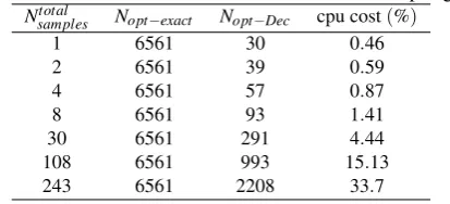
Table 6: Test case 3 with different number of samplings.

N_samplestotal Nopt−exact Nopt−Dec cpu cost(%)

1 6561 30 0.46

2 6561 39 0.59

4 6561 57 0.87

8 6561 93 1.41

30 6561 291 4.44

108 6561 993 15.13

243 6561 2208 33.7

7.1.4 Decomposition: test case 4 Spacecraft

The Decomposition technique is here applied to the minimisation of the mass of a spacecraft, as shown in Figure 7. The system is composed of three sub-systems, whose model can be found in this paper.Alicino and Vasile(2014a) The mass of the Attitude and Orbit Control System (AOCS),

MAOCS, is the sum of the mass of the reaction wheelMrw

and magneto-torqueMmag. The same two components give

the total power consumptionPAOCS: MAOCS=Mrw+Mmag

PAOCS=Prw+Pmag (47)

0 50 100 150 200 250 300

objective function

0 0.2 0.4 0.6 0.8 1 1.2

Belief

exact Belief samples in the left samples in the right

Figure 6: Test case 3. Belief curves generated with a fixed number of samples taken in two different parts of the partial belief curves.

Figure 7: Schematic of spacecraft sub-systems

The Telemetry and Telecommand System (TTS) is composed of an antenna, with massMant, a set of amplified

transponders, with mass Mamp, and a radio frequency

distribution network (RFDN), with massMr f dn. The total

mass and power requirement of the TTS is:

MT TC=Mant+Mamp+Mr f dn PT TC=Pamp

(48)

The AOCS and TTS submit their power requirements to the Electrical Power System (EPS). The EPS is composed of a solar array, a battery pack, a power conditioning and distribution unit (PCDU). The total mass of the power system is:

MEPS=Msa+Mbatt+Mpcdu (49)

The mass of each element of the power system is a monotonic function of the power requirement. The power requirement is the sum of thePAOCSandPT T S. Therefore,

are coupled variables and their effect manifests through

PT T SandPAOCSrespectively.

In this model, the design vector consists of 10 components (dim(d)=10), while the uncertain vector has 16 components (dim(u)=16), out of which, 11 uncertain components influence one and only one of the functions, thus they are collected in the uncoupled vector:

    

   

u_un−c= (uAOCS,uT TC,uEPS) dim(uAOCS) =4

dim(u_{T TC}) =2

dim(uEPS) =5

The other 5 uncertain variables belong to the coupled vector:

    

   

uc= (uAOCS→T TC,uAOCS→EPS,uT TC→EPS) dim(uAOCS→T TC) =0

dim(uAOCS→EPS) =2 dim(uT TC→EPS) =3

As one could see in Figure 8, there is a unidirectional flow of information: AOCS influences EPS but on the other hand EPS’s variables are not input to the AOCS; similarly for TTC and EPS; Figure 8 explains that AOCS and TTC influence EPS respectively with their power requirement.

Figure 8: Decomposition of the spacecraft system

The results obtained by applying the decomposition algorithm are shown in Figure 9. The number of optimisations required to generate the approximated curve can be estimated to be:

Noptimisation=12+52Ns (50)

The computational cost for each approximation can be found in Table 7.

7.2 Surrogate Approach and Robust Trade-off

The surrogate method is here applied to test case 1. First we computed the error in the representation of the space of the

1.5 1.6 1.7 1.8 1.9 2 2.1 2.2

objective function 0

0.2 0.4 0.6 0.8 1 1.2

Belief

exact Belief 1 sample 9 samples 24 samples

Figure 9: Convergence for the Spacecraft’s Belief curve with different numbers of samples (1, 9 and 24).

Table 7: Test case 4

N_samplestotal Nopt−exact Nopt−Dec cpu cost(%)

1 65536 64 9.7656e−04

4 65536 220 0.34

9 65536 480 0.73

16 65536 844 1.29

20 65536 1052 1.61

24 65536 1260 1.92

maxima for different numbers of intervals per dimension (see Tab 8). As expected, as the number of intervals per dimension increases, the space of the maxima tends to a continuous function and the representation with the surrogate becomes more and more accurate.

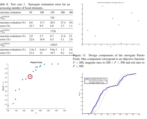
Then we addressed the solution of problem (44). The Pareto front in Fig 10 is the solution of problem (44). Each point along the curve was optimised using the surrogate to calculate the belief. Figure 11 show the design components of the elements in the Pareto Front.

Table 8: Test case 1. Surrogate estimation error for an increasing number of focal elements.

maxima evaluation 50 100 150 200 400

N_FEproblem 729

maxima evaluation (%) 6.8 13.7 20.5 27.4 54.8

error (%) 22.7 9.9 6.9 3.7 1.1

N_FEproblem 1728

maxima evaluation (%) 2.9 5.7 8.7 11.6 23.1

error (%) 22.6 10.9 6.5 5.1 2.9

N_FEproblem 15625

maxima evaluation (%) 3.2e-3 6.4e-3 9.6e-3 1.3 2.6

error (%) 21.2 12 10.7 8.2 4.4

Figure 10: Robust Pareto Front with Surrogate Model (test case 1)

evaluations also increases to a value that is anyway one order of magnitude lower than for a full calculation. 8 Conclusions

In this paper we introduced the concept of Evidence Network Models to represent complex engineering systems composed of a number of interconnected sub-systems. The uncertainty associated to each of the sub-systems and their interconnections is modeled with evidence theory. The calculation of the belief in the total value of the ENM is shown to be exponentially complex in the general case. Therefore, a decomposition algorithm is introduced to obtain an approximation in polynomial time. Furthermore, a surrogate-based approach is proposed to further reduce the computational cost when the belief needs to be maximised with respect to the decision (or design) variables.

The methodology is applied to a number of test cases, proving that, under suitable assumptions, a good approximation can be obtained at a fraction of the computational cost of an exact calculation. The paper

−5 −4 −3 −2 −1 0 1 2 3 4 −4

−3 −2 −1 0 1 2 3 4

Pareto Front’s distribution of the design vector d ∈ D

d

1

d2

Figure 11: Design components of the surrogate Pareto Front: blue component correspond to an objective function

F<200, magenta ones to 200<F<300 and red ones to

F>300.

0 50 100 150 200 250 300 350 400 450

0 0.1 0.2 0.3 0.4 0.5 0.6 0.7 0.8 0.9 1

F

Bel(F<

ν

)

exact Belief 3501387 f−eval Decomposition 242435 f−eval Surrogate 124881 f−eval

Figure 12: Comparison between the exact Belief curve and the reconstruction with the Decomposition and the Surrogate method. The legend includes the number of function evaluations in the three cases.

50 100 150 200 250 300 350 400 450

0 0.1 0.2 0.3 0.4 0.5 0.6 0.7 0.8 0.9 1

Exact curve 50 maxima evaluated 100 maxima evaluated 150 maxima evaluated 200 maxima evaluated 400 maxima evaluated

proposed also one theorem and two lemmas that proof that the approximated belief is always lower or equal to the exact one. This is a very important property as it provides a conservative expectation in the occurrence of an event or the truth of a proposition.

It was also shown that the method proposed in this paper allows for the fast estimation of the total belief of the network at a cost that is polynomial with the number of subsystems. This property is very important as it allows for an increases of the size and complexity of the system while maintaining the computation of the belief affordable. More work is required to study the behaviour of the ENM and estimation algorithms for different topologies and considering the full hyper-power set.

9 Acknowledgements

This work is partially supported by ESTECO Spa. and Surrey Satellite Technologies Ltd. through the project

Robust Design Optimization of Space Systems(European Space Agency - Innovation Triangle Initiative).

References

[Alicino and Vasile(2014a)] Alicino S, Vasile M (2014a) Evidence-based preliminary design of spacecraft. In: SECESA 2014

[Alicino and Vasile(2014b)] Alicino S, Vasile M (2014b) An evolutionary approach to the solution of multi-objective min-max problems in evidence-based robust optimization. In: 2014 IEEE Congress on Evolutionary Computation (CEC2014)

[Ortega and Vasile(2017)] Ortega C, Vasile M (2017) New heuristics for multi-objective worst-case optimization in evidence-based robust design. In: 2017 IEEE Congress on Evolutionary Computation (CEC2017) [Shafer(1976a)] Shafer G (1976a) A Mathematical Theory

of Evidence. (English). Princeton University Press [Shafer(1976b)] Shafer G (1976b) A Mathematical Theory

of Evidence. Princeton University Press

[Tardioli et al(2015)Tardioli, Kubicek, Vasile, Minisci, and Riccardi] Tardioli C, Kubicek M, Vasile M, Minisci E, Riccardi

A (2015) Comparison of non-intrusive approaches to uncertainty propagation in orbital mechanics. AAS Astrodynamics Specialists Conference, Vail, Colorado, USA AAS 15-545