City, University of London Institutional Repository
Citation:
Sahin, Ali (2016). Three essays in accounting. (Unpublished Doctoral thesis, City, University of London)This is the accepted version of the paper.
This version of the publication may differ from the final published
version.
Permanent repository link:
http://openaccess.city.ac.uk/17043/Link to published version:
Copyright and reuse: City Research Online aims to make research
outputs of City, University of London available to a wider audience.
Copyright and Moral Rights remain with the author(s) and/or copyright
holders. URLs from City Research Online may be freely distributed and
linked to.
THREE ESSAYS IN ACCOUNTING
by
ALI SAHIN
Thesis
Submitted to City University of London Sir John Cass Business School
for the degree of Doctor of Philosophy (PhD) in Accounting and Finance
Department of Finance
CONTENTS
List of tables 4
Acknowledgements 7
Abstract of the Thesis 8
Introduction 9
Chapter 1 Do analysts understand accruals’ persistence? Evidence revisited Abstract 12
1.1 Introduction 13
1.2 Literature review and Hypotheses 15
1.3 Data and sample selection 18
1.4 Empirical analysis 21
1.5 Sensitivity analyses 25
Appendix A 32
Tables 36
Chapter 2 How multi business segmentation affects the probability of meeting analysts’ earnings forecasts and economic consequences associated with it?
Abstract 50
2.1 Introduction 51
2.2 Literature review and Hypotheses 53
2.3 Data and sample selection 57
2.4 Empirical analysis 62
2.5 Sensitivity analyses 70
2.6 Conclusion 74
Appendix B 75
Tables 79
Chapter 3 Does unconditional accounting conservatism provide a rational explanation to B/P effect in stock returns?
3.1 Introduction 93
3.2 Literature review and Hypotheses 95
3.3 Data and sample selection 101
3.4 Empirical analysis and portfolio sorts 104
3.5 Sensitivity analyses 109
3.6 Conclusion 112
Appendix C 114
Tables 115
List of Tables
Chapter 1
Table 1.1 Descriptive statistics and correlations for ROA, accruals and conservatism
36
Table 1.2 Descriptive statistics and correlations for extended accrual decomposition
37
Table 1.3 Descriptive statistics for earnings forecast errors 38
Table 1.4 Correlations between analysts forecast errors, accruals and conservatism across 12 Months
39
Table 1.5 Regressions for forecast errors on total accruals and cash flows over 12 months
40
Table 1.6 Forecast errors and accrual components over 12 months
41
Table 1.7 Return regressions on cash flows (CF) and accruals (1976-2013)
43
Table 1.8 Forecast errors and accrual components on high/low conservatism portfolios
44
Table 1.9 Forecast error regressions on decile ranked accruals
45
Table 1.10 Forecast error regressions on high accrual
quintiles over the first 6 months
47
Table 1.11 Forecast error regressions on high/low total accrual (TACC) quintiles over the first 6 months
48
Table 1.12 Absolute forecast errors on Total Accrual (TACC) over the first 6 months
49
Chapter 2
Table 2.1 Descriptive statistics (Single vs Multi Segment firms) during 1999-2014
79
Table 2.2 Correlations-Pearson (above diagonal) and Spearman (below diagonal), 1999-2014
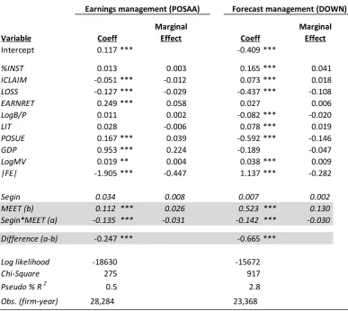
Table 2.3 Logit analysis of POSAA(DOWN) on MEET and Segin, 1999-2014
81
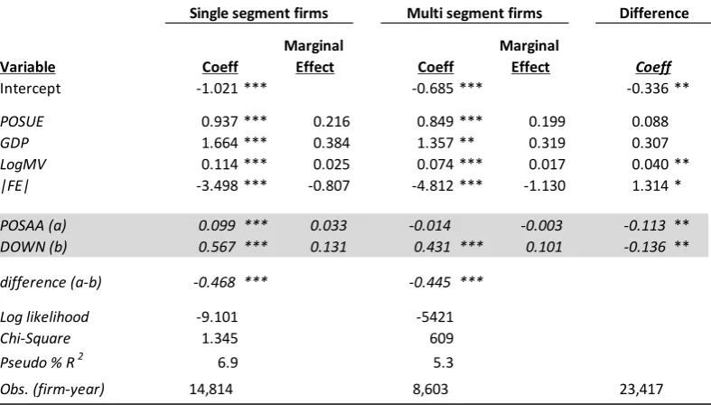
Table 2.4 Logit analysis of meeting probability (MEET) on POSAA(DOWN), 1999-2014
82
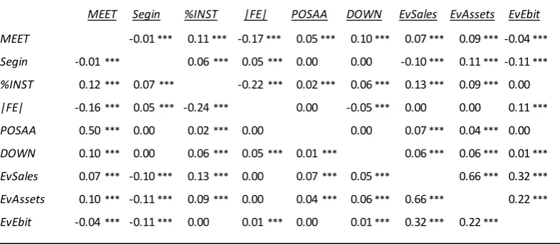
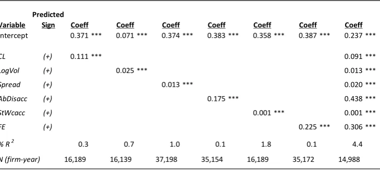
Table 2.5 Segment indicator regressions on information asymmetry proxies, 1999-2014
83
Table 2.6 Logit analysis of meeting probability (MEET) on information asymmetry
84
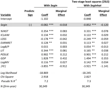
Table 2.7 Logit analyses of meeting probability (MEET) on Segin, 1999-2014
85
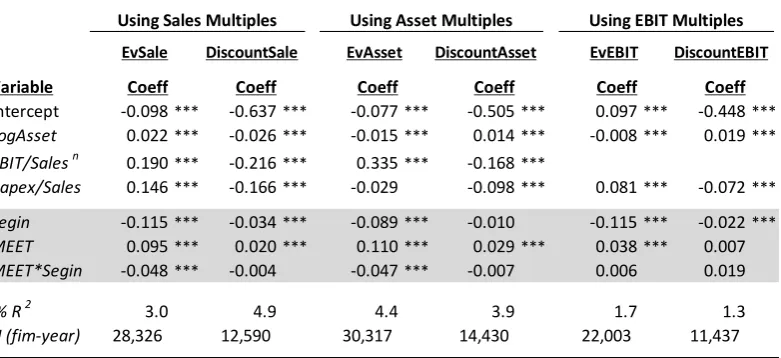
Table 2.8 Regressing EV and Discount (EV<0) on MEET and Segin, 1999-2014
86
Table 2.9 Regressing Excess Values (EV) on MEET and Segin by POSAA(DOWN), 1999-2014
87
Table 2.10 Returns regressions on MEET and Segin by POSAA(DOWN), 1999-2014
88
Table 2.11 Logit analysis of meeting probability (MEET) on POSAA(DOWN) separately, The effects of Institutional Ownership (INS), 1999-2014
89
Table 2.12 Logit analysis of meeting probability (MEET) on POSAA(DOWN) separately
90
Table 2.13 Logit analyses of meeting probability (MEET) on NofSeg, 1999-2014
91
Chapter 3
Table 3.1 Descriptive statistics for variables used in the analysis
115
Table 3.2 Correlation matrix—Pearson (above diagonal) and Spearman (below diagonal)
116
Table 3.3 Characteristics of HR/P portfolios with respect to other variables used in the tests
117
Table 3.4 Mean Annual Returns (%) to LTE/P and HR/P portfolios
118
Table 3.5 Mean Earnings Growth (%) to LTE/P and HR/P
portfolios
Table 3.6 Mean annual returns (%) to B/P and HR/P portfolios
120
Table 3.7 Mean Earnings Growth (%) to B/P and HR/P portfolios
121
Table 3.8 Mean Earnings Growth (%) to B/P and returns portfolios
122
Table 3.9 Mean Earnings Growth (%) to HR/P and returns portfolios
123
Table 3.10 Mean Annual Returns (%) to ALTE/P and HR/P
portfolios
124
Table 3.11 Mean Annual Returns (%) to LTE/P and
HR/NOA portfolios
125
ACKNOWLEDGEMENTS
This work would not have been possible without the help of a number of people.
First of all, I would like to take time to express my sincere and deepest gratitude to
my supervisor Ivana RAONIC, who has been a great mentor providing constant
support and encouragement from the very first meeting. I envy her patience and
greatly thankful for her insightful comments that improved the quality of my work.
I would also like to show my gratitude to Peter F. POPE whose wisdom and kind
support has immensely contributed to my knowledge and research. I am very
fortunate to have worked with him. I also wish to deliver my special thanks to Ian
MARSH, who has been most welcoming and approachable. His presence as a PhD
director has been a source of great comfort for all PhD students. I must also
acknowledge that I have received great support and kindness from the PhD office,
Malla PRATT and Abdul MOMIN. Finally, my wife, Ebru AKYEL SAHIN was a
huge inspiration to me. She encouraged me to undertake such a hard journey,
supported me endlessly and patiently from start to finish. I am extremely fortunate
ABSTRACT OF THE THESIS
INTRODUCTION
The first chapter of the thesis revisits the question whether analysts anticipate the persistence of accruals in future earnings. Previous research finds that accruals are
less persistent than cash flows, that investors fail to understand this property (e.g.,
Sloan, 1996), and also that analysts who provide information to investors do not
inform investors about the predicted future reversals of accruals (e.g., Bradshaw,
Richardson and Sloan, 2001). This research finds that analysts are overoptimistic
with respect to working capital accruals, and this is interpreted as their failure to anticipate accruals’ persistence. However, this interpretation is challenged by other
research findings. For instance, analysts’ forecasting abilities are praised by another
research (e.g., Fried and Givoly, 1982). There is also substantial evidence that
analysts can be strategic in their forecasts (e.g., Francis and Philbrick 1993), and
evidence indicates that traditional accrual definition omitting noncurrent operating
and financing activity accruals results in noisy measures of both accruals and cash
flows (e.g., Richardson, Soliman, Sloan, and Tuna, 2005). Therefore, we argue that analysts’ optimism with respect to working capital accruals might not be related to
their lack of sophistication, but due to incomplete accrual information. We give
consideration to ‘total accruals’ covering also noncurrent operating and financing
activity accruals, and revisit the issue.
Our results overall do not warrant the lack of sophistication argument; we find no
association between forecast errors and total accruals. Analysts seem to reflect predicted earnings reversals of total accruals in their forecasts. We also find strong evidence that analysts’ optimism with working capital accruals documented by
previous research is a result of analysts focusing on total accruals. Since accrual
components have different persistence degrees, and total accruals’ persistence is an average of its components’ persistence, it is likely that individual components are
associated with forecast errors if separately tested. Hence, a low persistent working
capital accruals may exhibit optimistic errors, while a high persistent financing
activity accruals pessimistic errors. Indeed, we find optimistic (pessimistic) forecast
errors with less (high) persistent accrual components, and no association between
forecast errors and middle persistent accrual components. Our results remain robust
The second chapter investigates whether multi segmentation affects the probability of meeting analysts’ forecasts, and whether the ‘diversification’ discount that multi
segment firms appear to suffer from is mitigated/exacerbated when multi segment firms meet/miss analysts’ forecasts. Analysis of this issue is important because previous research shows that meeting/missing analysts’ earnings forecasts leads to
premium/discount (e.g., Kasznik and McNichols 2002), and despite their obvious
importance in the economy, we lack evidence about the meeting/missing forecast
behaviour of multi segment firms. The subject becomes even more important given
the evidence that multi segment firms suffer from higher agency conflicts (traded
at discount, Berger and Ofek, 1995), and exhibit more complex information
environment (e.g., Bushman et al. 2004), both of which significantly affect also
meeting forecast probability (e.g., Matsumoto, 2002).
We argue that higher agency conflicts induce higher monitoring, and discourage multi segment firms’ managers from earnings/forecast management activity to meet
forecasts while more complex information environment leads to greater forecast
bias making forecasts harder to meet, and both will lead to lower probability of meeting analysts’ forecasts for multi segment firms. Our findings confirm these
expectations; multi segment firms exhibit less (no) earnings (forecast) management
activity to meet forecasts, more complex information environment and lower probability of meeting analysts’ forecasts relative to single segment firms.
We next test whether the ‘diversification’ discount is alleviated/exacerbated when multi segment firms meet/miss analysts’ forecasts. We argue that if the discount is
a results of higher agency conflicts, then meeting analysts’ forecasts does not
mitigate the discount. We also argue that investors will be aware that multi segment
firms show more complex information environment and use less earnings/forecast
management to meet forecasts. Hence, we expect that investors react less strongly
to meeting/missing forecasts by multi segment firms. Confirming this argument, we
find no evidence that meeting forecasts results in a premium in multi segment
setting, or that it reduces the diversification discount, while single segment firms experience significant premium (discount) when they meet (miss) forecasts.. We
management is used to meet forecasts implying that there are significant costs for
multi segment firms from engaging in these activities to meet forecasts.
The third chapter tests whether unconditional accounting conservatism provides a
rational explanation to book to price (B/P) effect in stock returns. Research shows
that stocks with higher ratios of fundamentals to price, i.e., high B/P tend to yield
higher future returns than stocks with lower ratios of fundamentals to price (e.g.,
(e.g., Graham and Dodd, 1934; Rosenberg, Reid, and Lanstein, 1985, Chan, Hamao,
and Lakonishok, 1991; Fama and French, 1992). Various explanations have been
brought forward to the phenomenon from both mispricing (e.g., DeBondt and
Thaler, 1985; Lakonishok, Shleifer, Vishny, 1994) and rational pricing of risk
perspective (e.g., Fama and French 1993), but challenged by subsequent evidence.
We offer a risk explanation using the mechanisms of unconditional accounting
conservatism following Penman and Reggiani (2013). In a pricing equation, a
risk-free earnings growth adds to price, while a risky growth adds to required return
rather than price making B/P ratio higher due to denominator effect. Accordingly,
a higher B/P corresponds to higher return. Conservative accounting produces such
risky growth (earnings are deferred under uncertainty producing earnings growth
that can be deemed at risk), and can explain the phenomenon.
We test the above argument within unconditional conservatism setting, which we
proxy by hidden reserves to price (HR/P) based on immediately expensed intangible
investments (Penman and Zhang, 2002).
We argue and find that HR/P is positively associated with both future returns and
subsequent earnings growth for any given B/P and long term earnings that we
construct to capture the risky earning growth following. Our paper makes several
contributions. We show unconditional accounting conservatism rationally explains
B/P effect in stock returns. We also show that stock market anomalies can be traced
within the accounting system, and by documenting that accounting conservatism is
a response to risk, and this risk perception aligns with the investors’ risk perception,
CHAPTER 1
Do analysts understand accruals’ persistence? Evidence revisited
Abstract
In this paper, we revisit the question whether analysts anticipate accruals’ predicted reversals (or persistence) in future earnings. Prior evidence shows that analysts are over optimistic with respect to working capital accruals, and this is interpreted as their inability to understand accruals’ persistence. However, using total accruals that cover also noncurrent operating and financing accruals as well as working capitals, we show that analysts’ forecast errors are uncorrelated with accruals. Since accruals have different components with different persistence characteristics, and total accruals reflects an average of its components’ persistence, it is likely that forecast errors are correlated with individual components if separately tested, but this does not indicate analysts’ lack of sophistication as long as analysts correctly anticipate total accruals. Consistent with this conjecture, we find low persistent accruals (e.g., working capital accruals) are optimistically, but high persistent accruals (e.g., financing accrual) pessimistically associated with forecast errors, while in the middle persistent, the association approaches zero. Overall these results do not warrant the analysts’ lack of sophistication argument.
Keywords: earnings/accrual persistence, analyst earnings/revenue forecast errors, efficiency
1.1. Introduction
In this paper, we revisit the question whether sell side security analysts anticipate the persistence (or predicted reversals) of accruals in future earnings. Analysis of
this issue is important, because evidence shows that accrual components of earnings
are less persistent than cash flows, investors do not seem to anticipate this property
(they experience negative future returns for buying high accruals, see Sloan, 1996),
and that analysts who provide information to investors also fail to inform them of
this accrual problem; Analysts are found to be overoptimistic with respect to high
working capital accruals (e.g., Bradshaw et al., 2001), and this is mainly interpreted
as their lack of necessary sophistication to fully understand accruals’ persistence.
However, this interpretation does not reconcile with other research findings. For
instance, analysts’ forecasting abilities are highly praised in another research; they
issue more accurate forecasts than earnings expectation models (e.g., Fried and
Givoly, 1982). There is also substantial evidence that analysts can be strategic in
their forecasts, which indicates their sophistication (e.g., Francis and Philbrick
1993). Finally, traditional accrual definition used in forecast error tests seems to
omit economically important accrual categories that can be highly relevant to
analysts (e.g., Richardson, Sloan, Soliman, and Tuna, 2005).
Therefore, we argue that analysts’ optimism with respect to working capital
accruals might not be due to lack of sophistication, but driven by incomplete accrual
information, hence give consideration to ‘total accruals’ suggested by Richardson
et al. (2005) covering also noncurrent operating and financing activity accruals.
Our empirical tests show no correlation between analysts’ forecast errors and total
accruals. Findings are robust to different samples, periods, specifications, decile
ranked accruals, high accruals, absolute forecast errors, controlling for cash flows
and high conservatism. We then decompose total accruals into components, and
repeat the same test for individual accrual components [to be comparable to these
tests, we also test the persistence degree of individual components as auxiliary, and
find that different components exhibit different persistence degrees with working
argue that if analysts focus on achieving minimum forecast error1, they should be
focusing on the accuracy of total accruals (given earnings= total accruals + cash flows), hence, it is highly likely that forecast errors may be correlated with individual accrual components that significantly deviate from the total accruals’
persistence (in individual cases associations maybe observed as previous research documents, but this does not indicate analysts’ not understanding of accruals’
persistence as long as total accruals are not associated with forecast errors). To be
precise, forecast errors can exhibit optimism (pessimism) with accrual components
that are less (higher) persistent than total accruals. Confirming, our argument, we
find that forecast errors are optimistically correlated with less persistent working
capital, but pessimistically correlated with higher persistent financial accruals while
with noncurrent operating accruals (having almost equal persistence as total
accruals with %74), the correlation is insignificant. Optimism in working capital
accruals is consistent with prior research, but we additionally show forecasts errors
to be pessimistically correlated with financial accruals, which also challenges to the notion that analysts’ overall optimism in earnings forecasts may stem from their
over optimism about current accruals.
Our paper makes several contributions to existing knowledge. Firstly, our findings
do not warrant analysts’ lack of sophistication argument with respect to accruals,
rather reinforce the evidence praising analysts’ forecasting abilities (e.g., Fried and
Givoly, 1982; Elgers and Murray, 1992). Secondly, our findings do not also support
the argument that analysts’ optimism in earnings forecasts may stem from accruals’
overestimation (analysts may intentionally collude with management and exhibit
optimism by inflating accrual expectations, but we find no such overestimation in
total accruals). Thirdly, although forecast errors are uncorrelated with total accruals,
we find that stock returns are negatively correlated, supporting the evidence in
Sloan (1996), who find that stock prices act as if investors fail to anticipate accruals’
persistence. Our findings also corroborate Elgers et al. (2001; 2003) findings; who
find that investors fail to efficiently impound all earnings relevant information contained in analysts’ forecasts. Finally, we find that the effect of conservative
1We assume that analysts’ ultimate objective is to achieve minimum forecast error given that the
accounting on accruals’ persistence is well understood by analysts, which provides
further support to their sophistication with respect to accruals.
The remainder of the paper is organised as follow. The next section provides
literature review and develops hypotheses. Section 1.3 describes the data, Section
1.4 explains research design and presents the results. Section 1.5 reports sensitivity
analyses and Section 1.6 concludes.
1.2. Literature review and hypotheses
1.2.1. Literature review
Evidence shows that earnings mean reverse (gradually decline in time), and accrual
components of earnings mean reverse quicker than cash flows, i.e., accruals are less
persistent2 than cash flows, but investors do not seem to anticipate this property.
Firms with high accruals are likely to experience lower earnings in future, and
investors without realising this property buy high accruals, and suffer from negative
stock returns (e.g., Sloan, 1996)3. This finding is important for analysts, because
they provide information to investors, and possibly affect their investment decisions
(Mendenhall, 1991). Hence, scholar also ask whether analysts inform investors
about this accrual problem, and by regressing forecast errors on past accruals, they
find analysts to be over optimistic with respect to working capital accruals (e.g.,
Bradshaw, Richardson and Sloan, 2001; Thomas and Zhang, 2002; Collins, Gong,
and Hribar, 2003; Elgers, Lo, and Pfeiffer 2001, 2003; Hanlon, 2005; Mashruwala,
Rajgopal, and Shevlin 2006; Drake and Myers, 2011), and this is interpreted as their
failure to anticipate the subsequent earnings declines associated with high accruals
consistent with the evidence in Sloan (1996).
However, this interpretation is not accommodated by other research findings. For
instance, analysts’ forecasting abilities are praised by another stream of literature;
they seem to provide superior and more accurate forecasts than estimates generated
by earnings expectation models (e.g., Brown and Rozeff, 1978; Fried and Givoly,
2Persistence indicates the continuity from one period to another. Evidence shows that earnings mean
reverse (gradually decline in time), and accruals mean reverse quicker than cash flows.
3 The is coined as accrual anomaly and explained by Sloan (1996) as investors’ fixation on reported
1982; Brown, Richardson, Schwager, 1987; Brown, Griffin, Hagerman, Zmijewski,
1987; Elgers and Murray, 1992). There is also growing evidence that analysts are
strategic in their forecasts indicating their sophistication (one cannot add bias into
a forecast without knowing the accurate one). Analysts issue optimistic forecasts to
curry favour with managers in order to obtain better access to private information,
to attract more investors and to boost investment banking fees, etc4. (e.g., Francis
and Philbrick 1993, Lin and McNichols, 1998; Teoh, Welch and Wong, 1998; Hong
and Kubik, 2003; Basu and Markov, 2004; Richardson, Teoh and Wysocki, 2004;
Cowen, Groysberg, and Healy, 2006; Raedy, Shane, and Yang, 2006; Teoh,
Groysberg, Healy, and Maber, 2011; Simon and Curtis, 2011). Evidence also suggests that analysts’ optimism in earnings is rational and originates in the loss functions underpinning analysts’ decisions (e.g., Gu and Wu, 2003; Basu and
Markov, 2004), which offers another challenge to lack of sophistication argument.
Finally, the accrual variable used in forecast error tests seems to be subject to
omitted information bias. Prior studies use working capital accruals assuming that they ‘do a better job’ in capturing accruals leading to earnings reversals. They argue
that accruals related to a number of special items (restructuring, impairments, equity
method losses, sale of plant/other investments, etc.) are nonrecurring, ‘tend to mean revert very quickly’ and ‘investors are more likely to anticipate’ their nature (e.g.,
Bradshaw et al., 2001). However, the evidence in Doyle, Lundholm, and Soliman
(2003) indicates that such “special” accruals are far from nonrecurring and relevant
to anticipate future stock returns. They show that firms with relatively large
omissions of such items in their definitions of pro forma earnings suffer from lower
returns. Similarly, Richardson et al. (2005) show that the accrual definition
proposed by Healy (1985) based on working capital excludes important accrual
categories, and results in noisy measures of both accruals and cash flows. They
document that the omitted parts of accruals (noncurrent and financial) also contain
measurement errors leading to significant security mispricing. For instance, great
subjectivity involves in the evaluation of noncurrent accruals (changes in tangible
4Analysts can also exhibit self-selection bias, i.e., they follow firms if they hold favourable views
intangible assets); capitalised interest expense5, write downs, depreciation amount,
etc., can restrict investors anticipating future economic benefits. There is also error
margin in the evaluation of financial accruals despite their higher reliability. Long
term investments and long term receivables can also be used to manipulate earnings.
1.2.2. Hypotheses
We argue that analysts’ optimism with respect to working capital accruals may not
be attributed to their lack of sophistication, but driven by incomplete accrual
information. Therefore, we focus on ‘total accruals’ in our analysis suggested by
Richardson et al. (2005) covering also noncurrent operating and financing accruals.
We assume that this broader accrual measure provides more powerful tests on
analysts’ sophistication regarding accruals as it hypothetically covers all relevant
accrual information available to analysts. Hence, if analysts lack the necessary
sophistication to understand accruals’ persistence, their forecast errors (realized
earnings minus forecast earnings) will also be associated with total accruals as
observed in previous research. Then we expect
H1: Analysts’ forecast errors are negatively correlated with current total
accruals.
On the other hand, if analysts fully understand accruals’ persistence, we expect6
H1A: Analysts’ forecasts errors are not correlated with current total accruals
Richardson et al (2005) disaggregate total accruals into components, and rate each
accrual category according to its reliability (reliability is determined by the degree
of measurement error the category involves). They find that less reliable accruals
lead to lower earnings persistence, and significant security mispricing, i.e., as the
persistence of an accrual component decreases it becomes harder to predict
5 Interest expense charged to assets (capitalised) transforms it into an operating item. There are also
similar transitions between operating and financing activities, and omitting this information possibly results in some relevant information loss to explain future earnings.
6There is also another alternative that analysts may collude with management to be optimistic by
(forecasting difficulty increases). They also find that working capital accruals are
less persistent than financial accruals (they explain this as working capital to be
subject to more measurement errors due to items containing subjective estimates
such as allowances for bad debts while financial items are mainly measured at fair
values). A related set of studies also finds that analysts issue more optimistic
forecasts for firms whose earnings are more difficult to predict (Das, Levine, and
Sivaramakrishnan, 1998, Ke and Yu, 2006), and that the difficulty of forecasting earnings interacts with analysts’ incentives to be optimistic which in turn, results in
optimistically biased forecast (Bradshaw, Lee, and Peterson, 2016). Therefore, if
the lack of sophistication argument holds, we expect
H2: Analysts’ forecast errors become more (less) optimistic as the persistence of an accrual component decreases (increases)
However, if the alternative holds (analysts fully understand accruals’ persistence),
analysts will focus on the accuracy of total accruals (since higher accuracy in total
accruals hypothetically leads to minimum forecast error given earnings=total accruals + cash flows). Accordingly, it is highly likely that forecast errors can be correlated with individual components whose persistence significantly deviate from total accruals’ persistence, and this will not indicate analysts’ lack of sophistication
as long as H1A holds (no association between forecast errors and total accruals). Therefore, given Richardson et al (2005), who find that working capital (financial)
accruals exhibit the lowest (highest) persistence among accrual components, and
that total accruals reflect an average of its components’ persistence, we expect, as
an alternative to H2,
H2A: Analysts’ forecast errors are optimistically (pessimistically) correlated with less (higher) persistent accruals, while in the middle
persistence, they approach zero.
1.3. Data and sample selection
In the data selection process, we follow Bradshaw et al. (2001) and Richardson et
al. (2005). We use non-financial US firms for the period between 1976 and 2013.
forecast data is from the IBES summary statistics file and stock returns data are
from CRSP daily files. To decompose accruals into components we rely on the
accrual definition from Richardson et al. (2005) 7:
TACC = ΔWC +ΔNCO + ΔFIN (1)
where TACC denotes total accruals, ΔWC is the change in noncash working capital,
ΔNCO is the change in net noncurrent operating assets and ΔFIN is the change in
net financial assets. TACC is further decomposed into its underlying components:
𝑇𝐴𝐶𝐶 = ∆𝐶𝑂𝐴 − ∆𝐶𝑂𝐿⏟ ∆𝑊𝐶
+ ∆𝑁𝐶𝑂𝐴 − ∆𝑁𝐶𝑂𝐿⏟ ∆𝑁𝐶𝑂
+ ∆𝑆𝑇𝐼 + ∆𝐿𝑇𝐼 − ∆𝐹𝐼𝑁𝐿⏟ ∆𝐹𝐼𝑁
(2)
Where ΔCOA (ΔCOL) denotes current operating assets (liabilities), ΔNCOA
(ΔNCOL) noncurrent operating assets (liabilities), and ΔSTI, ΔLTI and ΔLFINL short term investment, long term investment and financial liabilities respectively.
All variables are defined in Appendix A. Following Richardson et al. (2005), the
missing data on short term debt, investment and advances, long term debt, preferred
stock and short term investments are set to zero, while other missing observations
are eliminated from the analysis. Earnings variables (accruals and cash flows) are winsorised to +1 and -1 and deflated by average assets, while all other continuous
variables (e.g., earnings forecast errors) are winsorised to 1% and 99% to eliminate
the extreme observations. Following Bradshaw et al. (2001), we define earnings
forecast errors, Ferror, as the analysts’ consensus earnings forecasts minus the actual earnings provided by IBES deflated by share price from CRSP. We perform our tests across 12 months starting from the initial analysts’ forecasts, which are
generally issued in the first month after the prior period earnings announcement
date. Our final sample contains 48,142 firm-year observations per month.
1.3.1. Descriptive statistics and correlations
Table 1.1 Panel A reports descriptive statistics for earnings (ROA), total (TACC), working capital (ΔWC), noncurrent (ΔNCO) and financial (ΔFIN) accruals. It also
7 Richardson et al. (2005) define accrual-based earnings through the definition of net assets: Accrual
includes descriptive statistics for conservatism proxies, Hidden_reserves and
C_Score. Mean TACC is 0.051 or roughly 5% of total assets. Means of ΔWC and
ΔNCO are positive while mean ΔFIN is negative, which is indicative of an average
firm increasing its non-current operations, and financing this increase by net debt.
Panel B reports pairwise correlations, and reveals that all accrual components are
positively correlated with ROA, with ΔWC having the highest correlation. The positive correlation between ΔWC and ΔNCO suggests that they grow together. Both ΔWC and ΔNCO are negatively correlated with ΔFIN, in line with the suggestion that growth in operating activities is largely financed by debt.
Table 1.2 reports the descriptive statistics and pairwise correlations for the extended
accrual decomposition. Panel A shows that mean values of all accrual components
are positive with ΔNCOA (change in non-current assets) having the highest mean (0.055) while ΔLTI (change in long term investments) the lowest (0.002) suggesting that non-current operating accruals constitute the major part of accruals. Standard
deviations show that much of the variation in working capital accruals is attributed
to ΔCOA. Similar pattern is found with respect to ΔNCOA implying that the asset side of operating of accruals is more likely to be subject to measurement error. In
contrast, much of the variation in ΔFIN can be attributable to ΔFINL (financial liability). These observations suggest that the variation in operating accruals are
driven by assets, while the variation in financial activity accruals are driven by
liabilities. Panel B reports pairwise correlations and shows strong correlation
among accrual components. In particular, the positive correlation between ΔCOA and ΔCOL suggests that a growing (shrinking) business generally results in an increase (decrease) in both current operating assets and liabilities. There is also a
positive correlation between ΔCOA and ΔFINL suggesting that current operations are not only funded by operating liabilities, but also by financial debt. Moreover,
ΔNCOA is positively correlated with all liability accruals8
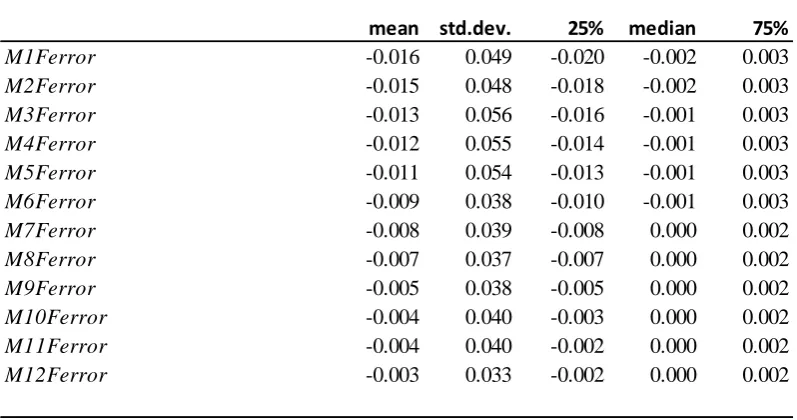
Table 1.3 reports the descriptive statistics of forecast errors across 12 months, and
shows negative means consistent with the prior evidence that analysts are optimistic
on average. It also shows that mean errors (and standard deviations) are gradually
8 Note that the liability component of accruals is substracted from the asset component to arrive at
disappearing as the earnings announcement date approaches (while initial earnings
forecast error is 1.6% of the share price, the last month forecast error is only 0.3%
of the price). This trend is expected, since the arrival of new information (e.g.,
quarterly earnings announcements) prompts analysts to revise their forecasts and
forecast errors decrease gradually.
Table 1.4 Panels A and B report Pearson correlations between forecast errors,
accrual components and conservatism proxies, and show that forecast errors are not
correlated with total accruals, but optimistically (pessimistically) correlated with
operating (financial) accruals. Similar pattern is observed for the extended accrual
components providing an initial support to H1A and H2A:
1.4. Empirical Analysis
1.4.1. Forecast error regressions on total accruals (TACC)
To test H1 (H1A), we use forecast error model by Bradshaw et al. (2001) employing total accruals (TACC), and extend the model by breaking TACC into components.
We conduct regressions using ordinary least squares (OLS) and cluster standard
errors by firm and year following Petersen (2009)9. We also use Fama and MacBeth
(1973) procedure that estimates annual cross sectional regressions and reports the
time series average of the resulting coefficients. The regressions are run for 12
consecutive months and also incorporate cash flows (CF) following Drake and Myers (2011), who argue that accruals and cash flows are the primary components
of earnings and that they are highly correlated.
𝐹𝑒𝑟𝑟𝑜𝑟𝑠,𝑖𝑡+1 = 𝛽0+𝛽1𝑇𝐴𝐶𝐶𝑖𝑡+ 𝛽2𝐶𝐹𝑖𝑡+ 𝜀𝑖𝑡+1 (3)
9 The method deals with the potential time and firm effects that can be present in panel data. Firm
Where Ferror denotes earnings forecast errors calculated as analysts’ forecasts of earnings minus actual earnings. While H1 requires a negative coefficient on TACC, the alternative hypothesis H1A requires insignificant coefficient on TACC.
Table 1.5 Panels A and B (without and with cash flows) present the results for
Equation (3). Both panels confirm H1A: analysts’ forecasts errors are not correlated with current TACC (the inclusion of CF does not alter the result). The coefficients on TACC are statistically and economically zero across all 12 months and t-stats are far below the thresholds.10
1.4.2. Forecast error regressions on accrual components
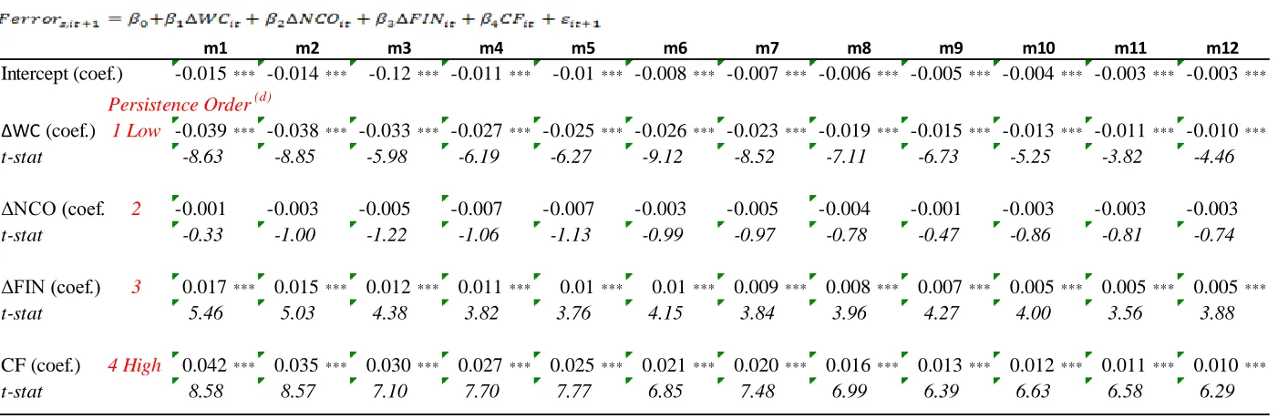
To test H2 (H2A), we next conduct the same analysis with the initial and extended accrual decompositions by fitting the following models:
𝐹𝑒𝑟𝑟𝑜𝑟𝑠,𝑖𝑡+1 = 𝛽0+𝛽1∆𝑊𝐶𝑖𝑡+ 𝛽2∆𝑁𝐶𝑂𝑖𝑡+ 𝛽3∆𝐹𝐼𝑁𝑖𝑡+ 𝛽4𝐶𝐹𝑖𝑡+ 𝜀𝑖𝑡+1 (4)
𝐹𝑒𝑟𝑟𝑜𝑟𝑠,𝑖𝑡+1 = 𝛽0+ 𝛽1𝛥𝐶𝑂𝐿𝑖𝑡+ 𝛽2𝛥𝐶𝑂𝐴𝑖𝑡+ 𝛽3𝛥𝑁𝐶𝑂𝐿𝑖𝑡+ 𝛽4𝛥𝑁𝐶𝑂𝐴𝑖𝑡
+𝛽5𝛥𝐿𝑇𝐼𝑖𝑡+ 𝛽6𝛥𝐹𝐼𝑁𝐿𝑖𝑡+𝛽7𝛥𝑆𝑇𝐼𝑖𝑡+ 𝛽8𝐶𝐹𝑖𝑡+ 𝜀𝑖𝑡+1 (5)
Where ΔWC +ΔNCO + ΔFIN=TACC. A negative (positive) sign on coefficients indicates forecast optimism (pessimism)11. Before running Equations (4) and (5),
to be comparable to these tests, we also run persistence tests for individual accrual
components following Richardson et al (2005). Reported in Appendix A panels A,
B and C, these tests show that CF has the highest persistent among earnings components with %80, while ΔFIN with %79 (0.791-0.002), ΔNCO with %74 (0.791-0.051), TACC with %73 (0.797-0.068), and ΔWC with %67 (0.791-0.122). This confirms accrual components exhibiting different persistence characteristics, and
TACC reflecting an average of its components’ persistence. Hence, if the lack of
10 Note that panel B shows pessimistic errors with CF, which has the highest persistent among
sophistication argument holds H2 will prevail. Since forecasting difficulty increases in less persistence, analysts will exhibit greater bias, and optimistic forecast errors
will increase as the persistence of an accrual component decreases, and vice versa (e.g., β1ΔWC< β2ΔNCO< β3ΔFIN< 0).
However, if analysts fully understand accruals’ persistence, then H2A will hold.
Forecast errors will be correlated with individual accrual components deviating
from total accruals’ persistence, i.e., errors can be optimistically (pessimistically)
correlated with working capital (financial) accruals, while in the middle persistent, they will approach zero (e.g., β1ΔWC< 0, β2ΔNCO=012, β3ΔFIN > 0). We acknowledge
that the confirmation of H2A will only support the argument of analysts fully understand accruals’ persistence if the H1A also holds, i.e., if there is no correlation
between forecast errors and TACC.
Table 1.6 reports the results for Equations (4) and (5) in Panels A and B. Confirming
H2A, both panels show that forecast errors are optimistically correlated with low persistence accruals, but pessimistically correlated with high persistence accruals
across 12 months, while the accruals of the medium persistence do not show any
association with errors (e.g., β1ΔWC=-0.039, β2ΔNCO=0, β3ΔFIN >=0.017 for month 1).
Moreover, the coefficient magnitudes in Panels A and B of Table 1.6 line up closely
with the relative persistence rankings reported in Appendix A Panels B and C (e.g.,
persistence degrees respectively are ΔCOL=%62.9 (0.803-0.177), ΔCOA=%66.8,
ΔNCOL=%70.6, ΔNCOA=%72.6, ΔLTI=%74.4, ΔFINL=%75.1, and ΔSTI=%76.9,
and their coefficients in forecast errors tests are ΔCOL=-0.062, ΔCOA=-0.037,
ΔNCOL=-0.031, ΔNCOA=-0.002, ΔLTI=0.006, ΔFINL=0.024, and ΔSTI=0.010.
F-tests confirm that the coefficients are different from each other).
In sum, both tests reported in Tables 1.5 and 1.6 confirm H1A and H2A and reject
H1 and H2, i.e., analysts’ forecasts errors are not correlated with current total accruals, and analysts’ forecast errors are optimistically (pessimistically) correlated
with less (higher) persistent accruals, while in the middle persistence, they approach
12 The persistence of ΔNCO is highly close to the persistence of TACC (%74 and %73), hence we
zero, these results indicate that analysts lack of sophistication argument with respect to accruals’ persistence is unwarranted.
1.4.1. Additional notes on empirical findings
When all accrual components are combined, they form total accruals (TACC), and we show that forecast errors are not correlated with TACC. We interpret this observation as analysts correctly anticipating accruals persistence, which is
plausible since accruals exhibit predicted reversals (Appendix A panels A, B and C
show that accrual components exhibit inherent persistence characteristics, i.e.,
components’ persistence degrees are not random, but can be predictable).
Richardson et al (2005) attribute these inherent properties to their degree of
reliability, which can be explained by the measurement errors they involve.
The fact that analysts correctly anticipate accruals’ persistence, does not also mean
that analysts are entirely correct in all their earnings estimates. There can be still
forecast errors explained by other factors such as strategic reasons and specific firm
characteristics, etc. Our results eliminate only one option, accruals.
We use actual EPS provided by IBES when examining analyst forecast accuracy.
Reported EPS is entered into the database on the same basis as analysts’ forecasts,
and by and large corresponds to earnings that represents core business activities as
opposed to net income (and may be quite different from the net income). Hence,
the database is considered to be the closest match with analysts’ forecasts. Evidence
also shows so. For instance, Bradshaw and Sloan (2002, p.41) find that ‘there has been a dramatic increase in the frequency and magnitude of cases where “GAAP” and “Street” earnings differ’. They also find that ‘market response to the Street
earnings number has displaced GAAP earnings as a primary determinant of stock prices’. See also, Ramnath, Rock, and Shane (2008) and Brown (2007) for studies
that use IBES EPS when investigating analyst forecast accuracy, analyst forecast
revisions, capital market reaction to earnings surprises published after 1990.
However, we have also performed forecast error tests using the Fully Reported
Bradshaw et al. (2001) use decile ranked accruals focusing on high/low magnitude
of accruals following Sloan (1996), who argues that accruals anomaly (negative
returns to past accruals) is caused by investors buying high accruals. However,
Richardson et al. (2005) findings indicate that the persistence rather than the
magnitude may drive security mispricing. They show that more measurement errors
lead to lower persistence, and lower persistence results in less predictability. This
implies that high magnitude does not always translate into more forecast errors, on
the contrary, low magnitude but low persistence (e.g., working capital accrual) can
cause greater forecast bias. Supporting this argument, Kraft, Leone, and Wasley
(2006) revisiting the accrual anomaly also show that it may not be the accruals’
magnitude that drives stocks mispricing, and Xie (2001) shows that investors
overprice the portion of abnormal accruals stemming from managerial discretion
(managerial discretion that adds greater measurement errors to accruals). Since the
persistence degree depends on measurement error, we consider more appropriate to
use actual values in our tests (decile ranking instead aims to eliminate measurement
errors). Nevertheless, our results remain robust to also decile ranked accruals, and
high/low accrual portfolios (reported in Tables 1.9, 1.10, and 1.11).
1.5. Sensitivity analyses
1.5.1. Future stock returns, accruals anomaly and analysts
Our first sensitivity test focuses on the associations between future stock return and
current accruals to examine whether investors and analysts exhibit the similar
behaviour in using accrual information. Even though, the evidence suggests that
investors follow analysts (e.g., Bartov and Mohanram, 2014), there is also strong
evidence that they use public information in different manners. Elgers et al. (2001,
2003) find that average investors make more accrual related error compared to
analysts, and give delayed response to more accurate analyst’ forecasts.
Hence, we predict investors to naively ignore the persistence of TACC and be negatively surprised by the subsequent earnings declines resulting in negative future returns as opposed to analysts’ zero TACC related error (there will be a
persistence decreases, i.e., investors will experience greater negative returns with
less persistent accruals, and vice versa. To test these predictions, we use the
following returns models
𝑅𝑒𝑡𝑖𝑡+1 = 𝛽0+ 𝛽1𝐶𝐹𝑖𝑡+ 𝛽2𝑇𝐴𝐶𝐶𝑖𝑡+ ∑𝑘𝑗=1𝛿𝑗𝑋𝑖𝑡+𝜀𝑖𝑡+1 (6)
𝑅𝑒𝑡𝑖𝑡+1 = 𝛽0+ 𝛽1𝐶𝐹𝑖𝑡+ 𝛽2𝛥𝑊𝐶𝑖𝑡+ 𝛽2𝛥𝑁𝐶𝑂𝑖𝑡+ 𝛽2𝛥𝐹𝐼𝑁𝑖𝑡 +
∑𝑘𝑗=1𝛿𝑗𝑋𝑖𝑡+𝜀𝑖𝑡+1 (7)
Where Ret denotes annual buy and hold stock returns for firm i at time t+1 adjusted by size and market returns. The accumulation starts in the fourth month after the
fiscal year end, and continues for 12 months. We control for firm size, market Beta, B/P, E/P and past returns following prior research (e.g., Fama and French, 1993).
Table 1.7 reports the results of Equations (6) and (7), and confirming our prediction
shows negative correlation between future returns and TACC (as opposed to analysts, who exhibit zero forecast error in TACC), while the coefficient on CF is statistically insignificant13.. In addition, we observe increasing investor optimism
as the accrual component’s persistence decreases, i.e., investors experience greater
(less) negative returns with less (high) persistent accruals consistent with Sloan
(1996), who documents stock prices act as if investors fail to anticipate accruals’
persistence. These findings overall show that analysts do a better job in anticipating
accruals’ persistence implying their relatively higher degree of sophistication. This
evidence also corroborates Elgers et al. (2001; 2003) who find that investors fail to
efficiently use earnings relevant information contained in analysts’ forecasts.
Note, even though we find that average investors seem to exhibit relatively less
sophistication than analysts in using accrual information, Lev and Nissim (2006,
p.193) show that the magnitude of accruals related trading is becoming small. ‘By
13Note, in a pricing equations, CF is used to calculate firm value; if it is correctly predicted, with a
and large, institutions shy away from extreme accruals firms’. They also show that
individual investors too are unable to profit from trading on accruals information
because of high information and transaction costs associated with implementing a
consistently profitable accruals strategy.
1.5.2. Accounting conservatism on earnings forecasts errors
Evidence shows, transitory shocks to earnings due to high conditional conservatism
lead to lower persistence of earnings (Konstantinidi, Kraft, and Pope, 2016) and
that analysts’ forecast bias becomes greater with high conditional conservatism
(Helbok and Walker 2004)14. Evidence also shows that intangible investments
immediately expensed due to unconditional conservatism result in more volatile
earnings (e.g., Kothari, Laguerre, and Leone, 2002; Amir, Guan, and Livne, 2007).
These findings suggest that in the presence of high conservatism, earnings become
less predictable. Therefore, we also test whether analysts anticipate accruals’
persistence under high conservatism, which would provide further evidence about
their sophistication. We use Hidden_reserves (Penman and Zhang 2002) and
C_Score (Khan and Watts, 2009)15 to proxy unconditional and conditional conservatism respectively (see Appendix A for definitions).
To distinguish between firms with high versus low unconditional (conditional)
conservatism, we group the sample into quintiles based on the magnitude of
Hidden_reserves (C_score) for the first three months before the quarterly earnings announcement, and use the following model.
𝐹𝑒𝑟𝑟𝑜𝑟𝑠,𝑖𝑡+1 = 𝛽0+𝛽1𝐶𝐹𝑖𝑡+ 𝛽2𝐷 + 𝛽3𝑇𝐴𝐶𝐶𝑖𝑡+ 𝛽4𝐷 ∗ 𝑇𝐴𝐶𝐶𝑖𝑡+ 𝜀𝑖𝑡+1 (8)
14Under conditional conservatism book values are written down when the news is bad, but not written up when the news is favourable (Basu, 1997). Under unconditional conservatism however, accounting generates pervasive bias regardless of news (Pope and Walker, 2003; Beaver and Ryan, 2005). It is determined at the inception of accounting transaction, and gives rise to hidden reserves (unrecorded goodwill) by means of an immediate expensing of R&D and advertising expenditures.
15 The variable is derived using Basu’s (1997) measure of asymmetric timeliness of bad relative to
good news, 𝑋𝑖𝑡= 𝛽1+ 𝛽2𝐷𝑖+ 𝛽3𝑅𝑖𝑡+ 𝛽4𝐷𝑖𝑅𝑖𝑡+ 𝑒𝑖𝑡 where the asymmetric timeliness is measured
Where D, conservatism dummy, differentiates between low/high Hidden_reserve (C_score) firm-years taking 1(0) if the earnings forecast error is in the high (low) conservatism quintile.
The coefficient on TACC measures the average forecast errors for low conservative firm-year, while the coefficient on interaction term measures the average
incremental forecast error for high versus low conservative firm-year. We predict
insignificant coefficient on TACC(D*TACC) if analysts fully understand accruals persistence (i.e., H1A holds, forecasts errors are not correlated with current TACC), We do not expect conservatism to play a significant role in the association between
accruals and forecasts errors.
Table 1.8 reports the results for Equation (8), and confirms our expectations. The
coefficients on TACC (D*TACC) are insignificant (marginally significant at %10 for D*TACC in one month). These findings overall indicate analysts’ sophistication with respect to accruals. Notice that the coefficients on D for conditional conservatism are negative and significant consistent with Helbok and Walker
(2004), who show greater forecast error under conditional conservatism.
1.5.3. Decile ranked accruals
We replace actual values of accruals with their decile ranks in the forecast error
regressions (3), (4) and (5) following Bradshaw et al. (2001). Each year, we rank
firms into deciles by the magnitude of accruals from low to high, and scale them to
(0,9) range so that lowest (highest) accrual firm years are assigned to 0 (9). The
scaling is used to alleviate nonlinearities in the data, and minimize the effects of
measurement errors.
The intercept in the decile rank regressions measures the average forecast error for
a low accrual firm year, while the coefficient on the accrual rank measures the
average incremental forecast errors for a high versus a low accrual firm year. If analysts’ understanding of accruals’ persistence is affected by the magnitude, we
should observe significant negative correlations between forecast errors and high
et al. (2001). However, we find the same pattern observed in Tables 1.5 and 1.6 that
confirm the alternatives, H1A and H2A.
Table 1.9 Panels A, B and C report the results of forecast error regressions on past
decile ranked accruals for Equations (3), (4), and (5), and confirm H1A that forecasts errors are not correlated with total accruals, and H2A forecast errors are optimistically (pessimistically) correlated with working capital (financing activity)
accruals, while in the middle persistence, forecast errors approach zero.
1.5.4. High/low accruals
We repeat the forecast error test for only the high accrual portfolios. Specifically,
each year, we rank firms into five quintiles from low to high by the magnitude of
accruals, and run Equations (3), (4), and (5) only with the high accrual portfolios.
We run these regressions for the first six months. Reported in Table 1.10 Panel A
and B, the results further confirm the hypotheses H1A and H2A.
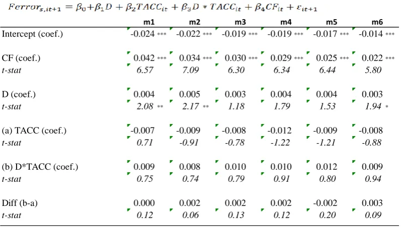
We also run forecast errors on high and low TACC portfolios. Each year we rank firms into five quintiles from low to high by the magnitude of TACC, then assign a dummy, D of 1 (0) to the high (low) TACC portfolios and run Equation (3) in the following form.
𝐹𝑒𝑟𝑟𝑜𝑟𝑠,𝑖𝑡+1 = 𝛽0+𝛽1𝐷 + 𝛽2𝑇𝐴𝐶𝐶𝑖𝑡+ 𝛽3𝐷 ∗ 𝑇𝐴𝐶𝐶𝑖𝑡+ 𝛽4𝐶𝐹𝑖𝑡+ 𝜀𝑖𝑡+1 (9)
D differentiates between low/high accruals. This method excludes middle quintiles from the test and keeps only the highest/lowest quintiles. Hence, the coefficient on
the TACC measures the average forecast error for the lowest TACC firm year, while the coefficient on the interaction term measures the average incremental forecast
errors for a high versus a low TACC firm year. Table 1.11 reports the results for Equation (9) and confirms H1A; insignificant coefficients on both TACC and
D*TACC (in some months marginally but pessimistic coefficients on D).
1.5.5. Absolute forecast errors and accruals
There are high correlations (some in opposite ways) among accrual components as
correlation between forecast errors and TACC, i.e., whether in the aggregate the opposite signed errors cancel each other’s effect on forecast errors. We also run
Equation (3) with absolute forecast errors to test this question. This method
eliminates the above possibility, but may lead to other problems such as the deviations both in the covariates’ coefficients and R2. Hence, the interpretation of
the results is limited to certain circumstances.
Since we use absolute values, a negative(positive) coefficient on accruals will now indicate analysts’ pessimism(optimism) contrary to signed error tests. Hence, with
absolute errors, we should observe a positive coefficient on TACC, if analysts lack the necessary sophistication, otherwise (with other signs) H1 will be rejected.
Table 1.12 reports the results for Equation (3) using absolute forecast errors for the
first six months, and shows significant negative coefficient on TACC. A negative sign means analysts’ pessimism, which rejects H1. Forecast errors should not
decrease as accruals increase in magnitude, just the opposite is expected, if the lack
of sophistication argument holds. Although, a significant coefficient on TACC does not confirm H1A too, it does not reject it either. Hence, we conclude saying ‘analysts’ lack of sophistication argument is unwarranted.
1.5.6. Other sensitivity analyses
We also performed forecast error tests using the Fully Reported (GPS) instead of
Actual IBES EPS. Forecast errors are calculated as Analyst Forecast of Earnings
minus the Fully Reported GPS and tests are run for the first six months. When using
the GPS, forecast errors seem to be optimistically correlated with both cash flows
and TACC, while optimism is greater with cash flows (e.g., the coefficient on TACC
is -0.029 while the coefficient on TACC is -0.115 and F-tests shows the coefficients are different from each other). This observation is inconsistent with both previous
research and with the theory. Therefore, we do not tabulate these results since using
Fully Reported (GPS) is unlikely to provide better outcome, and may even cause
greater noise and mislead the inferences
Our findings are also robust to Fama and MacBeth (1973) procedure, but we report
series regressions do not provide correct standard errors for autocorrelation in the
long term (stocks have weak time-series autocorrelation in daily and weekly
holding periods, but higher autocorrelation over long horizons, see Fama and
French, 1988). For alternative methods of correcting standard errors for time series
and cross-sectional correlations, we find appropriate to use Petersen (2009).
Other unreported tests which control for regulatory changes such as the enactment
of Regulation Fair Disclosure and the Global Analyst Research Settlement in 2002
reveal that the main findings remain robust. Regressions are also run by controlling
industry fixed effects using Fama and French industry classifications and for
different time periods such as using data post 1993 to test whether the main findings alter after the change in IBES’s method of calculating earnings (Konstantinidi et al.
2016). Our results remain robust also to these tests.
1.6. Conclusion
This paper revisits the question whether analysts anticipate the persistence of
accruals in future earnings. Previous research finds that accruals are less persistent
than cash flows, that investors fail to understand this property, and also that analysts
also fail to inform investors about this accrual problem. However, this research uses
working capital accruals to arrive that conclusion and substantial evidence indicates
that such accrual definition excluding noncurrent operating and financing activity
accruals can be subject to omitted information bias. Therefore, we use total accruals
in our analysis that covers the omitted parts of accruals, and revisit the issue.
Our results show that there is no correlation forecast errors and total accruals, and
that forecast errors increase in both highest and lowest persistent accrual
components while in the middle persistent, forecast errors approach zero. This
confirms our conjecture that analysts focus on total accruals’ accuracy (since
accruals components have different persistence degrees, and total accruals reflect
an average of its components’ persistence, it is plausible that individual components
are associated with forecast errors, but this will not indicate analysts’ lack of sophistication to anticipate accruals’ persistence as long as forecast errors
samples and model specifications, and therefore, our findings overall do not warrant
the lack of sophistication argument.
Appendix A
Variable definitions
Ferror Analysts’ earnings forecast errors computed as actual EPS from
IBES for year t+1 minus analysts’ consensus (median) forecast EPS from IBES in month s (s=1, 2, 3, ….12) scaled by price from CRSP in the first month year t earnings is announced. Ferror s, t+1 = [Actual EPS t+1 –Forecast EPS s, t+1] / P1,t
ROA Earnings. Operating income after depreciation (Compustat Item
OIADP, #178) deflated by average assets (Compustat Item AT, #6)
TACC Total accruals is the change in non-cash assets - change in liabilities deflated by average assets (Compustat Item AT, #6)
CF Cash flows (Compustat Item OANCF, #308) from operating
activities deflated by average assets.
ΔOPAC Operating accruals: change in non-cash working capital (ΔWCt) plus change in net non-current operating assets (ΔNCOt), deflated by average assets.
ΔWC Working capital accruals is the change in net working capital = WCt
- WCt-1. WC is current operating assets (COA) less operating liabilities (COL). COA=current assets (Compustat Item ACT, #4) - cash and short term investments (Compustat Item CHE, #1), and
COL=current liabilities (Compustat Item LCT, #5) - short term debt (Compustat Item DLC, #34).
ΔNCO Non-current operating accruals is the change in net non-current operating assets = NCOt - NCOt-1. NCO is = non-current operating assets (NCOA) - non-current op.liabilities (NCOL). NCOA=total assets (Compustat Item AT, #6) - current assets (Compustat Item ACT, #4) - investments and advances (Compustat Item IVAO, #32), and NCOL=total liability (Compustat Item LT, #181) - current liabilities (Compustat Item LCT, #5) - short term debt (Compustat Item DLC, #34) - long term debt (Compustat Item DLTT, #9)
ΔFIN Financing accruals is the change in net financial assets = FINt -FIN t-1. FIN=financial assets (FINA) - financial liabilities (FINL). FINA=short term investments (STI) (Compustat Item IVST, #193) + long term investments (LTI) (Compustat Item IVAO, #32). FINL= long term debt (Compustat Item DLTT, #9) + short term debt (Compustat Item DLC, #34) + preferred stock (Compustat Item UPSTKC, #130)
value-weighted average returns for all firms in the same size-matched decile. To form size deciles, market values are ranked annually, and assigned in equal numbers to ten portfolios.
E/P Earnings to price ratio calculated as operating income after depreciation (Compustat Item OIADP, #178) at time t deflated by market value at time t-1.
Size Natural log of market value of equity. Market value is calculated as the share price (Compustat item PRCC_F, #199) multiplied by common shares outstanding (Compustat item CSHO, #25)
B/P Book value of equity divided by market value of equity. Book value of equity = Common ordinary equity total (Compustat Item CEQ, #60) + Preferred treasury stock Current Assets (Compustat Item TSTKP, #227) + Preferred dividends in arrears (Compustat Item DVPA, #242)
Beta Estimated 60 month rolling regressions using the market model (𝑅𝑒𝑡𝑖𝑡 − 𝑅𝑓) = 𝛼 + 𝛽𝑖(𝑅𝑒𝑡𝑚𝑡− 𝑅𝑓) + 𝜖𝑖𝑡
Ret is the CRSP monthly buy and hold returns for 12 month for stock
i at time t, 𝑅𝑓 is risk the free rate, (𝑅𝑒𝑡𝑚𝑡− 𝑅𝑓) is the equity risk premium of the market portfolio. Rf is obtained from the US Federal Reserve, H15 report as the 10-year US Treasury bond rate for the relevant year. Retmt is the CRSP monthly value weighted return on a market portfolio cumulated over 12 months.
C_Score Firm specific conditional conservatism proxy varying across years developed using the following Khan and Watts (2009) model based on Basu (1997) asymmetric timelines of earnings measure;
𝑋𝑖𝑡 = 𝛽1+ 𝛽2𝐷𝑖+ 𝛽3𝑅𝑖(𝜇1+ 𝜇2𝑆𝑖𝑧𝑒𝑖+ 𝜇3 𝑀
𝐵𝑖
+ 𝜇4𝑙𝑒𝑣𝑖𝐷𝑖) +
𝛽4𝐷𝑖𝑅𝑖(𝛾1+ 𝛾2𝑆𝑖𝑧𝑒𝑖 + 𝛾3𝑀
𝐵 𝑖+ 𝛾4𝑙𝑒𝑣𝑖) + 𝛿1𝑆𝑖𝑧𝑒𝑖+𝛿2 𝑀
𝐵 𝑖+ 𝛿3𝐿𝑒𝑣𝑖+ 𝛿4𝐷𝑖𝑆𝑖𝑧𝑒𝑖+ 𝛿5𝐷𝑖𝑀
𝐵𝑖
+ 𝛿6𝐷𝑖𝐿𝑒𝑣𝑖 + 𝑒𝑖𝑡
The parameters are estimated annually, C_Score is calculated as 𝐶_𝑆𝑐𝑜𝑟𝑒𝑖𝑡 ≡ 𝛽4 = 𝛾1+ 𝛾2𝑆𝑖𝑧𝑒𝑖𝑡+ 𝛾3𝑀𝑖𝑡
𝐵𝑖𝑡
⁄ + 𝛾4𝑙𝑒𝑣𝑖𝑡