1417
Volume 66 141 Number 6, 2018
WHAT IS THE TRUE EFFECT OF
REBALANCING – A HIGHER
RETURN OR A LOWER RISK?
Martin Boďa
1, Mária Kanderová
11 Quantitative Methods and Information Systems Department, Faculty of Economics, Matej Bel University in
Banská Bystrica, Národná 1, 974 01 Banská Bystrica, Slovak Republic
To cite this article: BOĎA MARTIN, KANDEROVÁ MÁRIA. 2018. What is the True Effect of
Rebalancing – a Higher Return or a Lower Risk? Acta Universitatis Agriculturae et Silviculturae Mendelianae Brunensis, 66(6): 1417 – 1430.
To link to this article: https: / / doi.org / 10.11118 / actaun201866061417
Abstract
The paper is motivated by the fact that rebalancing in portfolio management has an effect recognisable with both return and risk, although its purported ambition is to control (or decrease) portfolio risk. Focusing upon rebalancing strategies in quadratic tracking, the paper investigates whether rebalancing contributes to higher returns or lower risks. The investigation is conducted as a case study of tracking the S & P 500 Index by means of its constituents in four different time periods spanning from 2011 to 2017. Different approaches to stock pre‑selection (according to investment styles induced by market capitalization and the P / B ratio), portfolio nominal sizes (ranging between 10 and 30 stocks) and rebalancing (including periodic, deviation or no rebalancing at all) are considered. The results suggest that the effect of rebalancing is generally more apparent with return and less with risk, and that risk may in times of turbulent markets be aggravated by rebalancing interventions.
Keywords: periodic rebalancing, deviation rebalancing, return, volatility, stock screening on size and multiples, quadratic tracking
INTRODUCTION
The problem of portfolio selection is primarily concerned with finding a selection of assets that warrants for the investor the maximum attainable (mean) return at a minimum risk. Before making the investment decision, the investor must take into account several factors such as risk, expected return, liquidity or transaction costs. Whenever a portfolio is chosen through the specification of asset weights, its optimality is challenged over the course of time. As the market environment changes, so do the return‑risk features of the portfolio change and the portfolio ceases to be optimal. In order to assure that the portfolio’s return‑risk features remain consistent over the entire investment horizon, the portfolio
deviation rebalancing, revisions are implemented wherever the portfolio return or risk deviates much from a pre‑set threshold. Nonetheless, any revision means a change in both the portfolio return and volatility. All in all, the actual effect of rebalancing is uncertain and the ambition of the paper is investigate whether the effect is more recognizable on return or risk. Needless to say, one would expect that rebalancing introduces a higher (mean) return and / or a lower risk, albeit this need not be necessarily so.
In this intent, the paper centres upon a small investor who desires to create a tracking portfolio that would be capable of copying or improving the performance of a suitable chosen market index. This small investor is willing to monitor his tracking portfolio continuously and is prepared to make revisions of its composition on a periodic basis or whenever there is a discrepancy from the desired development. For convenience, the investigation of rebalancing effects is accomplished empirically via a case study of the US stock market. The convenience of this choice rests in the fact that the US stock market is considered developed and liquid, and enjoys the reputation of a functioning financial market. In this set‑up, the research design aims at tracking the S & P 500 Index on the basis of the well‑known quadratic formulation, and considers as many as four investment styles for portfolio pre‑selection (i.e. investing only into big or small cap assets, an investing into value and growth assets) and nominal portfolio sizes of 10, 15, 20, 25 and 30 constituent stocks of the S & P 500 Index. These choices furnish the investigation with some amount of robustness and increase credibility of the comparison that is made: the buy‑and‑hold strategy of no rebalancing over a two‑year investment period is compared against four periodic rebalancing strategies (every month, 3 months, 6 months and 12 months) and four deviation rebalancing strategies (with deviation thresholds at 2.5 %, 5.0 %, 7.5 % and 10.0 % of the portfolio value). The effects of these investing / rebalancing strategies are studied for four consecutive and overlapping periods (datasets) that each consisted of a two‑year in‑sample horizon (used in portfolio choice) and a two‑year investment horizon (used for portfolio holding and rebalancing). These periods labelled as “20112014” to “20142017”.
Using a monthly frequency of data, the paper thus compares the return‑risk profiles of 720 tracking portfolios under different choices in different investment periods and accounts for the presence of transaction costs that are otherwise an inescapable element of investing, and examines how returns (measured by mean return) and risks (measured by volatility) change between the buy‑and‑hold strategy, four periodic and four deviation rebalancing strategies. The results are rather inconclusive and varied. Yet, it is found that rebalancing is more desirable in terms of return than risk in comparison to no rebalancing. Out of the rebalancing strategies
considered, period rebalancing strategies seem to be most contributive to the performance of tracking portfolios as they are seen in higher returns and smaller risk.
The rest of the paper is made up of four more sections. The following section describes rebalancing strategies and clarifies usefulness of rebalancing for the investor. It further summarizes and explains methodological technicalities employed in the design of the case study. The other section gives a detailed description of the case study and presents the results. One large tabular output is postponed to Appendix A. Eventually, the last section is concluding and contributes in terms of discussion.
MATERIALS AND METHODS
Dichtl et al. (2013) surveyed empirical studies in rebalancing and divided rebalancing strategies into two main groups: periodic rebalancing and deviation (interval) rebalancing. Periodic rebalancing strategies reallocate assets on a regular basis whereas deviation rebalancing reallocates assets only when there is a deviation from the desired development. There are several benefits associated with rebalancing. First, Dichtl et al. (2013) emphasize its ability to reduce risk considerably in comparison to the buy‑and‑hold strategy, but it fails to increase mean return (or it increases mean returns only by a slim margin). Second, Bouchey et al. (2012) and Willenbrock (2011) point out that rebalancing decreases risk concentration and downside risk. They assert that if the portfolio is well diversified from scratch, after a time it may become more concentrated (less diversified) on account of market trends. If the investor rebalances the portfolio during the investment horizon, he may avoid unnecessary concentration and the portfolio remains well diversified over the whole investment period.
are linear and benefits of rebalancing are quadratic, at a certain point rebalancing benefits will outweigh transaction costs and rebalancing will become desirable.
Rebalancing is not found uniformly recommendable as its net effects may depend on market trends and market volatility. For instance, Perold and Sharpe (1988) state fairly logically that rebalancing is most suitable for volatile markets without permanent rises or declines. On trendless markets rebalancing strategies are expected to bring about higher returns and reduce risk. This finding is also confirmed by Tokat and Wicas (2007) whose Monte Carlo experiments suggested that on trending markets rebalancing yields higher returns in comparison to less frequently rebalanced portfolios. On the other hand, their simulations show that on mean reverting markets a portfolio that was more frequently rebalanced exhibited a lower absolute return in comparison to a portfolio that was not rebalanced so frequently. In addition, the differences in risk between portfolios of different frequencies of rebalancing were relatively small, which follows from the fact that on mean reverting markets price rises are followed by prices falls, and so fluctuation of returns around mean return are quite moderate. Making use of US data for 1983 – 2012, Dayanandan and Lam (2015) examined whether there is a statistically significant difference in returns when different rebalancing strategies are employed in comparison to a non‑rebalanced portfolio (i.e. The buy‑and‑hold strategy). Their conclusion was that rebalancing strategies do not boost returns significantly except quarterly and semi‑annual rebalancing.
All these results indicate that it is not absolutely clear what the true effect of rebalancing really is‑whether it is to be seen in a higher mean return or a lower risk. This question becomes more apparent when even several rebalancing strategies are confronted. Here the investigation centres upon the buy‑and‑hold strategy, 4 periodic rebalancing strategies and 4 deviation rebalancing strategies to gain a better understanding how they perform and what they bring about.
Here the approach to portfolio selection is quadratic tracking of the underlying S & P 500 Index serving the role of a benchmark and is implemented here as a return‑based formulation (see formula (1) below). Return‑based portfolio tracking identifies the composition of the tracking portfolio by minimizing the discrepancy between historical tracking portfolio returns and benchmark returns. This discrepancy is expressed as tracking error variance that is nothing else but the mean square error. There are also extensions, e.g. Takeda et al. (2013) incorporated into the tracking task another factor that penalizes for great differences in weights of individual assets in the tracking portfolio. This leads to preferring portfolios that have almost uniform weights, and the authors maintain that this should warrant higher tracking accuracy
for the future. Sant’Anna et al. (2017) extended the objective function by an upper bound for absolute deviations between tracking portfolio and benchmark returns not to be exceeded over the in‑sample period. The reason for this upper bound is that large differences between portfolio returns in different periods should be avoided. On the other hand, value‑based formulations measure tracking error as a spread or distance between tracking portfolio values and benchmark values. These values are expressed in terms of historical trajectory and correspond to the values of the benchmark scaled by a constant factor such that the value at the end of the last historical period is equal to the value of the tracking portfolio.
Strub and Baumann (2018) call attention to disadvantages of both approaches as they claim that these approaches incur substantial transaction costs when rebalancing is accomplished periodically over the whole investment horizon. Value‑based formulations require more frequent rebalancing since rebalancing costs affect the distance betweeen trajectories only at the end of the in‑sample period and may be overcompensated by a reduced distance in the previous periods. To avoid these limitations, these authors proposed a new value‑based mixed‑integer linear programming formulation, which might be inspiration for further research.
the P / B ratio is just an indication of high growth potential. Conversely, value stocks are of those firms that attain lower earnings and are such that they preserve their market prices (and also value), which means the their P / B ratio must be relatively small. The procedure suggested by Fabozzi (1998, p. 60) for classifying stocks by value and growth is obeyed that consists in ordering stocks first by their P / B ratios and then dividing them into two classes by their accumulated market capitalization. Stocks whose accumulated market capitalization exceeds 50 % are treated as growth stocks (“G”) whereas those on the other side of the ordered axis are viewed as value stocks (“V”).
For presentational purposes, it is assumed that a sample of historical observations on benchmark returns and asset returns for assets pre‑selected for portfolio tracking is available. This historical sample consists of T historical observations of logarithmic returns of both the benchmark and some k pre‑selected assets. Let Y = (Y1, ..., YT)'
denote a (T × 1) vector of benchmark returns, let xt denote the vector of asset returns at any time t
(whereas t ∊{1, ...,T}) with elements xt = (xt,1, ..., xt,k)',
and eventually let X =(x1 | ... | xT)' denote a (T × k)
matrix of returns of the k assets that are to be represented in the tracking portfolio. The symbol ω
will stand for a (k × 1) vector of unknown portfolio weights w1, ..., wk that are obtained by minimizing
the following quadratic optimization problem (1)
in which 1 is a (k × 1) vector of ones. This general formulation of the optimization task allows an extension and can be complemented by the constraint banning short sales, i.e. w1, ..., wk ≥ 0.
This constraint is also employed here in the analysis as long‑only positions are sought, although also other constraints may be (and are) encountered in practice. Note that the expression to be optimized in (1) is just the mean square error and is called frequently tracking error variance (TEV). TEV is a non‑central measure and is thus influenced not only by random positive or negative deviations but also by underperformance or outperformance relative to the benchmark. A useful commentary on the computational aspects of (1) is provided by Rudolf et al. (1999).
Denote the moment of portfolio construction by the subscript τ (obviously satisfying τ ≥ T), denote the prices of individual assets at time τ by the symbols Pτ,1, ..., Pτ,k and the price of the benchmark as
Pτ,B. If the initial investment is Yτ, the following portfolio holdings are suggested: hτ,1 = Yτ∙w1 / Pτ,1, ...,
hτ,k = Yτ∙wk / Pτ,k. At the same time, a fictional
investment into the benchmark is done and the holding hτ,B = Yτ / Pτ,B is made. The symbol Y will
also denote the value of the tracking portfolio at any time denoted carefully in the subscript. Adding “B” in the subscript after the time instance will indicate
that the value of the benchmark investment is had in mind. Finally, assume that there is a percentage rate of transaction costs φ ∊ [0,1) that applies to the value of investment changes. Symbols that were introduced for a particular time extend naturally in their validity also for some future times. In consistency with the previous outline, there are several possibilities how to maintain this portfolio by the investor until the end of the investment horizon.
• The investor may choose not to revaluate the composition of the portfolio at all and opt for the buy‑and‑hold strategy. In such a case, transaction costs are incurred only at the moment of portfolio creation in the amount
i k
,i ,i i 1 h P ,
=
τ τ
=
ϕ
∑
⋅ (2)which reduces into φ ∙ Y when there is a ban on short sales (or when all holdings are positive). • Another possibility is to rebalance the portfolio
at regular time intervals of length, say, Dτ (Dτ > 0), no matter what the situation on the market is and how the tracking portfolio copies the index. In this case, at the next time τ + Dτ, the task presented in (1) is re‑solved with the updated data stored in Y and X. This updating is done on a sliding basis, keeping the length of observations to be T. New holdings are thus produced, hτ + Dτ, 1, ..., hτ + Dτ, k,
and the portfolio must be revised accordingly. In addition to the initial transaction costs resulting from the first portfolio construction given by (2), at the moment of revision, τ + Dτ, rebalancing transaction costs arise in the amount
i k
+ ,i ,i + ,i i 1 h h P .
=
τ Dτ τ τ Dτ
=
ϕ
∑
− ⋅ (3)This, of course, goes on a sliding basis at rebalancing times τ + Dτ, τ + 2Dτ, ... until the end of the investment horizon.
• Finally, another possibility is to set a threshold and to monitor discrepancy between the value of the tracking portfolio and the value of the investment into the benchmark. For this, some maximum tolerance threshold d (with d > 0) must be set. If at some future time τ + p (with p > 0) the situation |Yτ + p – Yτ + p,B | / Yτ + p,B > d first
happens to be the case, this is the impetus for an intervention and the portfolio is rebalanced. With this intervention portfolio, additional transaction costs are associated in the same manner as explained about the formula (3). However, one must bear in mind that to warrant consistency, it is necessary to rebalance also the index to the new value of the intervention tracking portfolio. Only then comparisons of values make sense.
here in the paper instead that there exists a separate account, from which these transaction costs are covered. Only the final value of the tracking portfolio is confronted with the volume of transaction costs (in an inflation‑free world), and the net value of the investment is computed by subtracting the transaction costs total from the portfolio value.
RESULTS
The analysis assumes that a small investor wishes to track the S & P 500 Index, which is a good informal descriptor of the US stock market. To maintain consistency of his tracking task, he considers in stock pre‑selection and later in portfolio selection only the basket of about 500 constituents represented in the index. Further, to control for the amount of transaction costs that will decrease his ultimate performance (e.g. non‑institutionalized and perhaps non‑advised), he is willing only to form a tracking portfolio of no more than 30 stocks. To this end, he uses 24 historical logarithmic returns of a monthly frequency for a period of two years (the in‑sample period) that are used in setting up portfolio weights by means of to the optimization model in (1). Having selected the optimal weights that minimize historical tracking error variance and seem to yield historically as close as possible the return‑risk profile of the benchmark S & P 500 Index, he creates a portfolio on the last day of the in‑sample period that coincides with year‑end. This portfolio is then held and monitored in the course of the next two years (the out‑of‑sample period or investment horizon) and as a result of this monitoring it may happen to be rebalanced, depending on the rebalancing strategy employed.
A total of four samples were created to move more towards generalizability and to ameliorate the effect of market trends. These samples (referred to later as “periods”) spanned a period of four years, with the first two years representing the in‑sample period of 24 monthly returns for portfolio selection and the last two years standing for the out‑of‑sample horizon of active investing and rebalancing. The samples started at 2011 (the start of the in‑sample period of Sample 1) and ended at 2017 (the end of the out‑of‑sample period of Sample 4). These samples are denoted in what follows as “20112014” to “20142017”.
The stock pre‑selection for each portfolio was rendered by the method of screening on size (market capitalization) and a multiple (the P / B
ratio) using the procedures detailed in the previous section. At the moment of portfolio creation the S & P 500 Index was screened for its constituents. The basket of effective constituents that could take part in the empirical investigation was limited by the availability of data. Some stocks represented in the index at the end of the in‑sample period did not have a sufficiently long history to be contained fully in the in‑sample and out‑of‑sample period. The reason being, some stocks were too fresh and were only newly added to the index in the in‑sample period, whilst others were relieved from the index during the out‑of‑sample period (e.g. in consequence of a merger). The available number of stocks according to the market capitalization and P / B ratio screening criteria for each sample is displayed in Tab. I. The effective basket of the S & P 500 constituents thus ranged from 450 (with period “20122015”) to 458 (with periods “20112014” and “20142017”).
Having considered 5 nominal portfolio sizes of 10, 15, 20, 25 and 30 stocks, all possible combinations were tagged by as “B10” to “B30”, “S10” to “S30”, “G10” to “G30”, and “V10” to “V30”. The meaning of these tags should actually be clear, e.g. “G15” is the situation in which 15 constituent stocks of the S & P 500 Index were selected that show the highest growth potential. In portfolio tracking, the initial investment was made at the end of the in‑sample period in the amount of US $ 10,000. Shorts sales were not permitted as well and the rate of transaction costs was set to φ = 0.4 % (this choice is not unconventional, e.g. Ionescu, 2002, Grobys, 2010).
As announced earlier, three kinds of rebalancing strategies were contrasted in total:
• The buy‑and‑hold rebalancing strategy, in which no revision is introduced into the portfolio composition over the whole out‑of‑sample period (investment horizon): Once the portfolio is created at the end of the in‑sample period, it remains intact and the only manipulation that is done with this portfolio that at the end of the out‑of‑sample period (investment horizon) its performance is measured and netted of the transaction costs incurred at the very inception. Their amount is represented by formula (2).
• Four periodic rebalancing strategies, in which revisions of the portfolio composition are undertaken periodically at regular time intervals regardless of whether it is actually necessary or not: The periodic revisions were introduced
I: Stocks available for investing identified by the screening across the samples
Number of stocks available Big caps („B“) Small caps („S“) Growth stocks („G“) Value stocks („V“)
Sample 1: period “20112014” 230 228 208 250
Sample 2: period “20122015” 233 217 216 234
Sample 3: period “20132016” 233 224 216 241
by every month (1M), every quarter (3M), every half‑year (6M) and every year (12M). Transaction costs are now higher and they include the transaction costs arisen at the inception of the portfolio in formula (2) and the transaction costs arisen regularly with every revision in formula (3).
• Four deviation rebalancing strategies, in which the portfolio is monitored at a monthly frequency and revisions are effected only when its value deviates significantly from the index upwards or downwards by a threshold d. The four thresholds specified here are d = 2.5 %, d = 5.0 %, d = 7.5 %, and d = 10.0 %. Thus, with threshold d = 2.5 % the portfolio is recomposed if whatever month its value deviates from the notional investment into the index by more than 2.5 %. Again, transaction costs are the sum of the transaction costs at the inception of the portfolio in formula (2) and the transaction costs arisen with every irregular revision in formula (3).
Notice that at the end of the out‑of‑sample period the portfolio was not actually liquidated and so transaction costs were spared. Only the terminal value of the portfolio was ascertained and adjusted by the total amount of transaction costs.
In sum, there were as many as 80 tracking portfolios constructed at the end of the in‑sample periods using the formulation of quadratic tracking (4 different samples × 4 different investment styles
× 5 nominal portfolio sizes) whose performance was further affected by the choice of one of the 9 rebalancing strategies (the “buy‑and‑hold strategy” plus 4 periodic rebalancing strategies plus 4 deviation rebalancing strategies). In total there were 80 × 9 = 720 portfolios with stratified performance and return – risk profiles.
In computations and preparing graphical presentations, the software R version 3.0.1 (R Core Team, 2013) was employed with several of its libraries, quantmod (Ryan et al., 2017), quadprog (Turlach and Weingessel, 2013), timeSeries (Wuertz and Chalabi, 2013) and PerformanceAnalytics (Peterson et al., 2014).
The results are in greater detail presented in Appendix A in a tabular format. The table organizes for the four periods and the 20 combinations of investment style and portfolio size five indicators of performance: mean return, volatility, mean active return, active volatility and net cumulative return. All these indicators are properly annualized (for volatilities using the traditional square‑root‑of‑time rule). Mean return and volatility measure the average (annualized) value of logarithmic tracking portfolio returns and their standard deviation over the entire out‑of‑sample period (investment horizon). The former is a measure of return of a tracking portfolio, whilst the latter is a measure of risk. Mean active return and active volatility
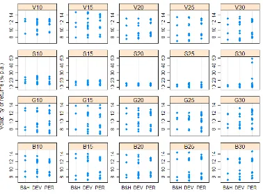
accomplish this measurement using logarithmic returns in excess of logarithmic benchmark returns (here returns of the S & P 500 Index) and measure thus return and risk of a tracking portfolio relative to the benchmark. Net cumulative return is the annual geometrically‑compounded average return after the deduction of transaction costs that arose at the inception of the portfolio and owing to its rebalancing. Theoretically, net cumulative return in comparison to mean return is more informative, but practically there are negligible differences between these two in the table of Appendix A. The table is prepared in such a way that it is possible to compare the return‑risk profiles of the buy‑and‑hold strategy and the rebalancing strategies. The indicators at the buy‑and‑hold strategy (B and H) are reported as they were observed, but for deviation and periodic rebalancing (DEV and PER) only averages are reported in order to conserve space. The values for mean return and volatility are further presented in Figs. 1 and 2 (the values are now for enhanced readability multiplied by a factor of 100 and expressed in percentages). Both figures show stripcharts that compare the mean returns and volatilities observed for the 20 combinations of investment style and portfolio size and for the buy‑and‑hold strategy (B and H) and two rebalancing strategies (DEV and PER) irrespective of the period. Every plotted point answers to one tracking portfolio.
The visualization of Figs. 1 and 2 suggests that there is not a compelling case in favour of any rebalancing strategy when compared to the buy‑and‑hold strategy as far as mean return or volatility is considered. The level and variability of mean returns and volatilities appear mostly much alike irrespective of whether the buy‑and‑hold strategy, periodic or deviation rebalancing is considered. Nonetheless, the stripcharts in Fig. 1 give a recurring impression that some configurations of rebalancing improve mean returns of the tracking portfolios in comparison to the buy‑and‑hold strategy. This is especially apparent for the investment styles “V”, “G” and “B” and the combination “S30”. A similar inclination of rebalancing strategies to increase volatility in some cases is discernible from the stripcharts in Fig. 2. This is especially true for the combination “S30” or “G30”. On the contrary, the combinations “B10” and “B15” are examples where rebalancing tend to decrease volatility.
The obtained results are evaluated by accounting for four explanatory factors of return and volatility: sample or period, investment style, nominal portfolio size and rebalancing style. A useful summary in this respect is presented in Tab. II that displays for each of these explanatory factors the percentage of cases when a rebalancing strategy was better than the buy‑and‑hold strategy. For example, with investment style “B” there were
II: Performance of the rebalancing strategies considered in comparison to the buy–and–hold strategy
Factor Proportion of preferable results
Mean return Volatility Net cumulative return
Style (B) 45.63 % 42.50 % 45.63 %
Style (S) 53.13 % 29.38 % 53.13 %
Style (V) 34.38 % 51.88 % 34.38 %
Style (G) 60.63 % 49.38 % 60.63 %
# assets = 10 38.28 % 38.28 % 38.28 %
# assets = 15 40.63 % 42.97 % 40.63 %
# assets = 20 57.03 % 40.63 % 57.03 %
# assets = 25 54.69 % 43.75 % 54.69 %
# assets = 30 51.56 % 50.78 % 51.56 %
Deviation strategy 36.56 % 33.75 % 36.56 %
Periodic strategy 60.31 % 52.81 % 60.31 %
Period (20112014) 51.25 % 60.63 % 51.25 %
Period (20122015) 41.25 % 40.00 % 41.25 %
Period (20132016) 36.25 % 25.00 % 36.25 %
Period (20142017) 65.00 % 47.50 % 65.00 %
III: Factors explanatory of the performance of the rebalancing strategies considered
Variable
Mean return
(% p.a.) Volatility (% p.a.) return (% p.a.)Mean active Active volatility (% p.a.) Net cumulative return (% p.a.)
LASSO BIC AICC LASSO BIC AICC LASSO BIC AICC LASSO BIC AICC LASSO BIC AICC
Style (B) 0.15 0.19 0.45
Style (S) 1.65 1.91 1.89 0.84 1.87 1.85 –0.49 1.25 1.75 1.75 Style (V) 5.13 4.93 4.93 –0.55 4.57 4.24 4.08
Style (G) 0.43 –0.31 0.53
# assets 0.06 0.05 0.05 0.01 –0.04 –0.04 0.05 0.05 0.00 –0.03 –0.03 0.06 0.04 0.04 Buy–and–hold
Deviation (0.025) Deviation (0.050) Deviation (0.075) Deviation (0.100)
Periodic (1M) 0.08
Periodic (3M) 0.63 1.23 0.17 0.54 0.40 1.19 0.48 0.51 0.58 1.66 1.66 Periodic (6M)
Periodic (12M) 0.04 0.28
Period (20112014) 15.71 16.65 16.59 8.53 10.75 10.69 1.77 14.62 16.01 16.11 15.93 17.45 17.45 Period (20122015) 1.75 2.69 2.62 10.16 12.38 12.32 –2.09 –4.28 –4.34 17.36 18.74 18.85 0.76 2.28 2.28 Period (20132016) 11.40 13.62 13.56 –3.27 –5.46 –5.52 18.02 19.41 19.51
Period (20142017) 6.39 7.33 7.27 7.97 10.19 10.13 –7.03 –9.23 –9.29 10.79 12.17 12.28 5.65 7.17 7.17 Adjusted R–square 0.85 0.85 0.85 0.95 0.95 0.95 0.49 0.50 0.50 0.98 0.98 0.98 0.82 0.82 0.82
Notes: 1) Blank cells indicate that respective parameters were not identified as qualifying for the fitted models and were not present in the regression specifications found optimal under LASSO or with respect to the BIC or AICC. 2) There is one numeric variable in the models (“# assets”) and three categorical variables that were transformed appropriately to dummy variables: “Style” (with four possible values “B” / ”S” / ”V” / ”G”), rebalancing strategy (“Buy‑and‑hold” plus four “Deviation” and four “Periodic” variations) and “Period” (covering nominal categories from “20112014” to “20142017”). Variables with nominal values ranging through several rows of the Tab. are separated by lines. In order to suppress the troubles associated with perferct collinearity, the intercept was omitted from considerations in search for the best model. each model.
merely 45.63 % portfolios (i.e. 73 portfolios) for which mean return was improved by rebalancing, 42.50 % occurrences (i.e. 68 portfolios) when volatility was smaller after rebalancing and again only 45.63 % cases (i.e. 73 portfolios) when net cumulative return was higher after rebalancing. Of course, this is in comparison to the buy – and – hold strategy where no revisions are made. Bold font at the percentages indicates a prevalence of cases. The incidences and frequencies of preferable results of rebalancing strategies are equal for both mean return and net cumulative return resulting in the respective columns of Tab. II being identical. This is but a consequence of the fact that there are factually minor differences between mean return and net cumulative return as can be deduced from Appendix A.
What is apparent is that volatility is not very improved by rebalancing for most of the factors considered. The buy‑and‑hold strategy seems to be universally more preferable in terms of volatility and whenever rebalancing on average improves volatility, it is not very convincing as the proportion of preferable results in comparison to the buy‑and‑hold strategy is not much greater than the threshold level 50 %. The only exception is the period “20112014” when there is a more compelling improvement of rebalancing in terms of volatility over non‑rebalancing. Otherwise, slight improvements of rebalancing over the buy‑and‑hold strategy are found for the investment style “V”, the nominal portfolio size 30 and periodic rebalancing.
More favourable towards rebalancing are the results concerning return of tracking portfolios no matter whether understood in terms of mean return or net cumulative return. In this regard, it is especially growth tracking portfolios and partly small‑cap tracking portfolios that are preferable over the buy‑and‑hold strategy, and then tracking portfolios of nominal size between 20 and 30 assets as well as periodically rebalanced portfolios. Rebalancing was also found more reliable in comparison to the buy‑and‑hold strategy in improving mean return and net cumulative return for the periods “20112014” and “20142017”.
It appears that periodic rebalancing is doubtless more desirable than deviation rebalancing as it is persuasive in increasing return (60.31 % cases in comparison to the buy‑and‑hold strategy) and decreasing volatility (52.81 % cases when drawn to comparison with the buy‑and‑hold strategy). It also seems that preferability of rebalancing strategies is also dependent on market trends that are embodied in samples or periods. The period “20112014” is characteristic of higher return and smaller volatility of rebalanced tracking portfolios (whereas the improvement in volatility is more conclusive), and the period “20142017” suggests the desirability of rebalancing strategies in terms of return only (yet, to a greater extent). In the other two period,
the buy‑and‑hold strategy fared overall better with respect to both return and risk.
In order to account for the factors that dominate in explaining the performance of the selected portfolios a search was initiated using traditional methods of regression model selection. Three competing approaches encompassed LASSO (for details see e.g. Tibshirani, 1996) and selections based upon the Bayesian information criterion (BIC) and the small‑sample corrected Akaike information criterion (AICC) (for details see e.g. Burnham and Anderson, 2002). Whereas LASSO houses its own approach to estimating the parameters (by least absolute shrinkage), in other cases the estimation method was OLS (ordinary least squares). The best models explaining mean return, volatility, mean active return, active volatility and cumulative return net of transaction costs (all of them treated in annualized form as percentages) are reported in Tab. VI with the associated adjusted R‑squared measures. In fitting, the results of individual datasets were merged into a larger dataset of 720 observations.
The selected regression models presented in Tab. III provide a varied picture in explaining the return‑risk profiles of the tracking portfolios constructed and rebalanced. Whereas BIC tends to identify a parsimonious specification, LASSO shows a tendency of overfitting for volatility, mean active return and net cumulative return. These observations may be inferred from the overview of Tab. III:
• The small‑cap investment style “S” appears to be most useful in improving mean return, mean active return and net cumulative return, whereas the value style “V” is obviously most contributive to risk irrespective of whether this is understood in terms of volatility and active volatility. In other words, small‑cap tracking portfolios are identified most recommendable in terms of return and value tracking portfolios are associated with higher risk.
• Portfolio size seems to boost return and generally reduces risk (in either case regardless of the measurement basis).
• Periodic rebalancing every three months is found sufficiently explanatory of all the five performance measures. It pushes towards higher return and higher risk. The former is as might be expected, whereas the latter is controversial.
CONCLUSION
According to many academic and empirical studies, the priority effect of rebalancing is decreasing portfolio volatility with differentiated consequences upon return. This claim is valid only when the aim of rebalancing is to preserve the return‑risk profile of the investor over the entire investment horizon and the portfolio is then reallocated toward the original return – risk preferences.
The paper investigated whether in quadratic tracking portfolio rebalancing is more discernible in a higher return or a lower risk. The design of the paper was empirical as it incorporated a case study of tracking the S & P 500 Index from the perspective of a small investor who is willing to create a portfolio of 30 equities at most represented in the S & P 500 Index. Several choices were accommodated to improve generalizability of findings concerning investment style, nominal portfolio size, type of rebalancing and period.
The evidence amassed by this empirical exercise is somewhat mixed and partly inconclusive as it is difficult to state firmly what effect rebalancing wields upon return and risk of tracking portfolios. The results are differentiated by investment style, portfolio size, rebalancing type and period, although the effect of rebalancing may be discernible more in increased returns than in decreased volatility of tracking portfolios in comparison to the buy – and – hold strategy. This is apparent from Tab. III. Nonetheless, it is 3 – month periodic rebalancing that has a positive effect upon return characteristics as well as an inflating effect upon risk characteristics of tracking portfolios, and the said effects are stronger when compared with the buy – and – hold strategy. The results established here are in conformity with the findings of Dichtl et al. (2013) who compared performance of various rebalancing strategies in a set – up of a similar case study using historical data and focusing upon US, UK and German markets. These authors concluded as well that quarterly period rebalancing yielded significantly higher returns than threshold rebalancing did. It becomes apparent that return and risk in rebalancing strategies go hand in hand. Higher returns are mostly compensated and downplayed by higher risk so rebalancing strategies cannot be effectively employed in controlling for lower risk as springs out of Tabs. II and III. The only exception is clearly periodic rebalancing strategies that translate into higher returns and smaller risk when put into comparison to the buy – and – hold strategy. Using US data, Dayanandan and Lam (2015) demonstrated similarly that there was no substantial difference between returns generated by various rebalancing strategies and returns generated by the buy – and – hold strategy except quarterly and semi – annual rebalancing. Their finding tallies again with the results of the present study.
When viewed through the prism of intuition and confronted with other studies (such as Dichtl et al., 2013; Bouchey et al., 2012), it is somewhat controversial to find out that rebalancing may inflate risk and does so indeed in many a case. The observation is possibly linked with phases through which the US stock market had to go over the investment horizons considered in the design of the case study. For individual years of each investment horizon and for the horizon itself, Tab. IV reports mean return and volatility of the S & P 500 Index and time – trending regression coefficients that indicate whether the index tended to rise or decline. These slope coefficients measure steepness of index values and come from traditional artificial time regression. Only the slope coefficient estimated for the yearly period 2015 was found insignificant since in that year the S & P 500 Index displayed a mixture of locally increasing and decreasing trends with no prevailing tendency.
The investment horizon in the period “20112014” displays high returns, the smallest volatility and a high slope coefficient, which is in line with the magnitude of regression coefficients in Tab. III. At that time, the market was calm and rebalancing strategies yielded favourable results in comparison to the buy – and – hold strategy on the scale of both return and risk as reads from Tab. II, which is
IV: Return, risk and trend development of the S & P 500 Index over the investments horizons considered
Yearly
period Mean return (p.a.) Volatility (p.a.) Slope Biperiod–annual Mean return (p.a.) Volatility (p.a.) Slope
2013 0.0216 0.0244 28.99***
2014 0.1079 0.0807 23.02*** 2013 – 2014 0.1836 0.0839 24.76***
2015 –0.0073 0.1351 –2.76ns 2014 – 2015 0.0503 0.1102 9.25***
2016 0.0911 0.1014 24.34*** 2015 – 2016 0.0419 0.1177 6.06**
2017 0.1775 0.0422 30.50*** 2016 – 2017 0.1343 0.0770 28.99***
Legend: The reported values are estimated from monthly data and converted to an annual frequency in a usual way. “Slope” is the regression coefficient identified by regressing values of the S & P 500 Index upon an artificially created time trend of values 1 to 12 (for yearly period) or 1 to 24 (for bi–annual period). The slope regression coefficients were estimated by OLS. The symbols at reported slopes are traditional labels for significances of regression coefficients: three asterisks “***” show significance at 0.001, two asterisks “**” indicate significance at 0.01 and the superscript “ ns“ signalizes
a finding in stark contrast to those by Perold and Sharpe (1988) and Tocat and Wicas (2007). The latter authors applied a somewhat different approach based on Monte Carlo simulations and observed that at steadily trending markets rebalancing produced a smaller return. On the other hand, their simulations suggested that differences in terms of risk between rebalanced and non – rebalanced portfolios were relatively negligible providing that markets were mean – reverting. A reversed situation similar to the period “20112014” is with the period “20142017” when again the market was calm and constantly trending upward. Nonetheless, then the effect was recognizable with returns only as attested by Tab. II, and not volatility.
All things considered, it may be said that the effect of rebalancing strategies is more pronounced upon return and less upon risk and that in the latter case the direction is not always as expected. All the same, this final summary observation must be taken with caution as the focus of the present study is highly selective and zooms in merely upon a fraction of the US stock market over a certain historical time frame using a few methodological choices, which is but a limitation shared by every case study of this sort. On one hand, it is therefore difficult to generalize and comment on general regularities. On the other hand, the case study provides evidence which challenges the dominant conviction that rebalancing chiefly reduces risk.
Acknowledgements
The support of a grant scheme of VEGA [# 1 / 0554 / 16] is acknowledged, and also usefulness of suggestions brought up by Andrea Kolková in discussing the first draft of the manuscript.
REFERENCES
BOUCHEY, P. et al. 2012. Volatility harvesting: Why does diversifying and rebalancing create portfolio
growth? Journal of Wealth Management, 15(2): 26 – 35.
BURNHAM, K. P. and ANDERSON, D. R. 2002. Model selection and multimodel inference: A practical
information‑theoretic approach. 2nd Edition. New York: Springer.
DAYANANDAN, A. and LAM, M. 2015. Portfolio rebalancing – hype or hope? Journal of Business Inquiry,
14(2): 79 – 92.
DE JONG, F. and DRIESSEN, J. 2013. The Norwegian government pension fund’s potential for capturing iliquidity
premiums. Report for the Norwegian Ministry of Finance. Available at: SSRN: http://dx.doi.org/10.2139/ ssrn.2337939 [Accessed: 2017, September].
DICHTL, H., DROBETZ, W. and WAMBACH M. 2013. Testing rebalancing strategies for stock‑bond
portfolios: What is the optimal rebalancing strategy? Applied Economics. 48(9): 772 – 788.
FABOZZI, F. J. 1998. Overview of equity style management. In: FABOZZI, F. J. (Ed.). Active equity portfolio
management. New Hope (PA): Frank J. Fabozzi Associates, pp. 57 – 70.
FAMA, E. F. and FRENCH, K. R. 1993. Common risk factors in the returns on stocks and bonds. Journal of
Financial Economics,33(1): 3 – 56.
IONESCU, G. 2002. Portfolio construction strategies using cointegration. Dissertation thesis. Bucharest: Academy of
Economic Studies Doctoral School of Finance and Banking.
GROBYS, K. 2010. Correlation versus cointegration: do cointegrated based index‑tracking portfolios perform
better? Zeitschrift für Nachwuchswissenschaftler, 1(2): 72 – 78.
MASTERS, S. J. 2003. Rebalancing. Journal of Portfolio Management, 29(3): 52 – 57.
PEROLD, A. F. and SHARPE, W. F. 1988. Dynamic strategies for asset allocation. Financial Analysts Journal,
44(1): 16 – 27.
PETERSON, B. G. et al. 2014. PerformanceAnalytics: econometric tools for performance and risk analysis. R package,
version 1.4.3541. [Online]. Available at: http://cran.r‑project.org/web/packages/Performance Analytics/ index.html [Accessed: 2017, September].
R CORE TEAM. 2013. R: a language and environment for statistical computing. Vienna: R Foundation for Statistical
Computing.
RYAN, A. J., ULRICH, J. M., THIELEN, W. and TEETOR, P. 2017. quantmod: Quantitative financial modelling
framework. R package, version 0.4‑12. [Online]. Available at: http://cran.r‑project.org/web/packages/ quantmod/index.html [Accessed: 2017, September].
RUDOLF, M., WOLTER, H.‑J. and ZIMMERMANN, H. 1999. A linear model for tracking error minimization. Journal of Banking & Finance,23(1): 85 – 103.
SANT’ANNA, L. R., FILOMENA, T. P., GUEDES, P. C. and BORENSTEIN, D. 2017. Index tracking with controlled number of assets using a hybrid heuristic combining genetic algorithm and non‑linear
programming. Annals of Operations Research, 258(2): 849 – 867.
STRUB, O. and BAUMANN, P. 2018. Optimal construction and rebalancing of index‑tracking portfolios. European Journal of Operational Research, 264(1): 370‑387.
TAKEDA, A., NIRANJAN, M., GOTOH, J. and KAWAHARA, Z. 2013. Simultaneous pursuit of out‑of‑sample
TIBSHIRANI, R. 1996. Regression shrinkage and selection via the Lasso. Journal of the Royal Statistical Society Series B, 58(1): 267 – 288.
TOKAT, Y. and WICAS, N. W. 2007. Portfolio rebalancing in theory and practice. Journal of Investing, 16(2):
52 – 59.
TURLACH, B. A. and WEINGESSEL, A. 2013. Quadprog: functions to solve quadratic programming problems. R
package, version 1.5‑5. [Online]. Available at: http://cran.r‑project.org/package =quadprog [Accessed: 2017, September].
WILLENBROCK, S. 2011. Diversification return, portfolio rebalancing, and the commodity return puzzle. Financial Analysts Journal, 67(4): 42 – 49.
WUERTZ, D. and CHALABI, Y. 2013. TimeSeries: Rmetrics ‑ financial time series objects. R package, version 3010.97.
[Online]. Available at: http://cran.r‑project.org/web/packages/timeSeries/index.html [Accessed: 2017, September].
Contact information Martin Boďa: [email protected]
St
rate
gy
Style and # asse
ts M ea n re turn V ola t M ea n ac ti ve re turn A ct iv e vo lat Ne t cu m re turn
Style and # asse
ts M ea n re turn V ola t M ea n ac ti ve re turn A ct iv e vo lat N et cu m re turn
Style and # asse
ts M ea n re turn V ola t M ea n ac ti ve re turn A ct iv e vo lat Ne t cu m re turn
Style and # asse
ts M ea n re turn V ola t M ea n ac ti ve re turn A ct iv e vo lat Ne t cu m re turn P eri o d 20112014 B a nd H B10 0. 1353 0.0945 – 0.0306 0. 1459 0. 1384 S10 0.2843 0. 1548 0. 1184 0.2070 0. 3131 G10 0. 1393 0.08 50 – 0.0266 0. 1284 0. 1428 V10 0. 128 7 0.08 86 – 0.0372 0. 1466 0. 1312 D EV 0. 1401 0.0948 – 0.0258 0. 1464 0. 1437 0.2779 0. 1521 0. 1120 0.2014 0. 3054 0. 1350 0.0910 – 0.0309 0. 138 1 0. 138 1 0. 1258 0.0929 – 0.0401 0. 1521 0. 1282 PE R 0. 1405 0.0920 – 0.0254 0. 1451 0. 1442 0.2903 0. 1557 0. 1244 0.2058 0. 3210 0. 1400 0.0946 – 0.0259 0. 1429 0. 1436 0. 1262 0.0926 – 0.0397 0. 1518 0. 128 6 B a nd H B15 0. 1616 0.0825 – 0.0043 0. 1345 0. 1675 S15 0.278 8 0. 158 5 0. 1129 0.2103 0. 3063 G15 0. 168 7 0.0797 0.0028 0. 1240 0. 1755 V15 0. 1523 0.078 7 – 0.0136 0. 1352 0. 1571 D EV 0. 1631 0.08 54 – 0.0028 0. 138 5 0. 1692 0.2764 0. 1557 0. 1105 0.2093 0. 3033 0. 1646 0.08 50 – 0.0013 0. 1321 0. 1708 0. 158 0 0.0820 – 0.0079 0. 1397 0. 1635 PE R 0. 1638 0.0899 – 0.0021 0. 1456 0. 1700 0.2574 0. 1348 0.0915 0. 18 58 0.28 00 0. 1594 0.08 71 – 0.0065 0. 1389 0. 1651 0. 1642 0.08 18 – 0.0017 0. 1417 0. 1705 B a nd H B20 0. 1442 0.08 52 – 0.0217 0. 1363 0. 1482 S20 0.2920 0. 1555 0. 1261 0.2142 0. 3228 G20 0. 1415 0.0916 – 0.0244 0. 1422 0. 1452 V20 0. 1662 0.08 38 0.0003 0. 1394 0. 1727 D EV 0. 1509 0.08 82 – 0.0150 0. 1407 0. 1556 0.2662 0. 1547 0. 1003 0.2107 0.2909 0. 1597 0.0928 – 0.0062 0. 1432 0. 1654 0. 1715 0.08 52 0.0056 0. 1410 0. 178 6 PE R 0. 1553 0.0898 – 0.0106 0. 1439 0. 1605 0.2595 0. 1479 0.0937 0.2034 0.2827 0. 1848 0.0895 0.0189 0. 1422 0. 1937 0. 1737 0.0847 0.0078 0. 1433 0. 18 11 B a nd H B25 0. 1278 0.0793 – 0.038 1 0. 1314 0. 1303 S25 0.2606 0. 1298 0.0947 0. 18 84 0.28 37 G25 0. 1741 0. 1053 0.0082 0. 1592 0. 18 16 V25 0. 1843 0.0841 0.0184 0. 1428 0. 1932 D EV 0. 1399 0.08 51 – 0.0260 0. 1396 0. 1435 0. 18 50 0. 1410 0.0191 0. 1920 0. 1947 0. 1762 0. 1053 0.0103 0. 1595 0. 1840 0. 18 17 0.08 54 0.0158 0. 1441 0. 1902 PE R 0. 1444 0.08 63 – 0.0214 0. 1413 0. 148 5 0. 1736 0. 1479 0.0077 0.2017 0. 18 18 0. 178 7 0.0996 0.0128 0. 1546 0. 18 69 0. 18 67 0.08 63 0.0208 0. 1458 0. 1959 B a nd H B30 0. 1542 0.08 84 – 0.0117 0. 1465 0. 1593 S30 0.2702 0. 1112 0. 1043 0. 1728 0.2956 G30 0. 1829 0.0922 0.0170 0. 1515 0. 1916 V30 0. 18 04 0.0896 0.0145 0. 1470 0. 18 87 D EV 0. 1643 0.0903 – 0.0016 0. 148 3 0. 1706 0.2382 0. 1391 0.0723 0. 18 87 0.2565 0. 1761 0.0928 0.0102 0. 1510 0. 18 38 0. 1825 0.0913 0.0166 0. 1490 0. 1912 PE R 0. 1618 0.0916 – 0.0041 0. 148 5 0. 1677 0.4311 0. 3266 0.2652 0. 3695 0. 5276 0. 1821 0. 1021 0.0162 0. 1607 0. 1907 0. 18 87 0.08 89 0.0228 0. 1470 0. 1982 P eri o d 20122015 B a nd H B10 0.0426 0. 1345 – 0.028 8 0. 1936 0.0416 S10 0.098 1 0. 1747 0.0267 0.238 1 0.098 6 G10 0.0534 0. 1319 – 0.018 0 0. 1928 0.0525 V10 0.0148 0. 1231 – 0.0566 0. 1924 0.0143 D EV 0.0231 0. 1245 – 0.048 3 0. 18 87 0.0225 0.0206 0. 1635 – 0.0508 0.2306 0.0209 0.0441 0. 1263 – 0.0273 0. 1895 0.0432 0.0249 0. 1266 – 0.0465 0. 1975 0.0242 PE R 0.0238 0. 1219 – 0.0475 0. 18 56 0.0231 – 0.0132 0. 1532 – 0.0846 0.2238 – 0.0126 0.0508 0. 1296 – 0.0205 0. 1930 0.0501 0.0339 0. 1270 – 0.0375 0. 198 7 0.0330 B a nd H B15 0.0461 0. 1294 – 0.0253 0. 1926 0.0452 S15 0.0339 0. 1293 – 0.0374 0. 1933 0.0331 G15 0.0482 0. 1384 – 0.0232 0.2000 0.0472 V15 0.038 5 0. 1189 – 0.0328 0. 1822 0.0376 D EV 0.0451 0. 1268 – 0.0262 0. 1943 0.0442 0.0066 0. 1327 – 0.0647 0. 1979 0.0069 0.0570 0. 1341 – 0.0143 0. 1970 0.0563 0.0375 0. 1219 – 0.0339 0. 18 73 0.0366 PE R 0.0512 0. 1258 – 0.0202 0. 1945 0.0504 – 0.0311 0. 1326 – 0. 1025 0.2012 – 0.0293 0.0720 0. 1350 0.0006 0. 1952 0.0715 0.0498 0. 1253 – 0.0216 0. 1916 0.0490 B a nd H B20 0.0438 0. 118 1 – 0.0276 0. 18 60 0.0429 S20 0.0421 0. 1226 – 0.0293 0. 1758 0.0411 G20 0.0262 0. 1321 – 0.0452 0. 1918 0.0254 V20 0.0405 0. 1118 – 0.0309 0. 1768 0.0396 D EV 0.0454 0. 1190 – 0.0260 0. 18 75 0.0445 0.038 8 0. 1261 – 0.0325 0. 18 59 0.0379 0.0390 0. 1217 – 0.0324 0. 18 58 0.038 1 0.0379 0. 1133 – 0.0335 0. 1777 0.0370 PE R 0.0463 0. 1241 – 0.0251 0. 1931 0.0455 0.0301 0. 1306 – 0.0412 0. 1906 0.0293 0.0795 0. 1236 0.008 1 0. 18 58 0.0791 0.0491 0. 1189 – 0.0223 0. 18 38 0.0482 B a nd H B25 0.0503 0. 1268 – 0.0211 0. 18 88 0.0493 S25 0.0736 0. 1126 0.0022 0. 1717 0.0731 G25 0.0479 0. 1208 – 0.0235 0. 1825 0.0469 V25 0.0658 0. 1125 – 0.0056 0. 1821 0.0651 D EV 0.0492 0. 1256 – 0.0221 0. 1901 0.0484 0.0847 0. 1015 0.0133 0. 1694 0.0847 0.0498 0. 118 7 – 0.0216 0. 18 18 0.0489 0.0672 0. 1131 – 0.0042 0. 1822 0.0665 PE R 0.0709 0. 1295 – 0.0005 0. 1895 0.0703 0.0568 0. 1059 – 0.0146 0. 1720 0.0561 0.0745 0. 1191 0.0031 0. 1848 0.0740 0.0548 0. 1171 – 0.0166 0. 18 69 0.0541 B a nd H B30 0.0327 0. 1278 – 0.038 7 0. 18 65 0.0318 S30 0.0691 0. 1135 – 0.0023 0. 1744 0.0684 G30 0.08 56 0. 118 1 0.0143 0. 18 33 0.08 55 V30 0.0393 0. 1147 – 0.0321 0. 18 05 0.0384 D EV 0.0402 0. 1204 – 0.0312 0. 18 57 0.0394 0.08 82 0. 1069 0.0168 0. 1748 0.08 84 0.0842 0. 1164 0.0129 0. 18 12 0.0841 0.0352 0. 1174 – 0.0362 0. 18 16 0.0343 PE R 0.0775 0. 1324 0.0061 0. 1965 0.0771 0.0652 0. 1126 – 0.0061 0. 178 3 0.0647 0.08 78 0. 1262 0.0164 0. 1905 0.08 78 0.0469 0. 1230 – 0.0244 0. 18 78 0.0460 No te : T he figur es r ep or
ted for the
buy – and – hold inves ting s tr at egy (“
B and H”) come as they wer
e ob
served, but those for the
devi
ation and p
erio di c r ebalancing s tr at egies (“ DE
V” and “PER
”, r esp ecti vel y) ar e a ver ag e v alues. T he figur es a t “ DE
V” arise as the
ari
thmeti
c a
ver
ag
e of four v
alues for the
four differ ent thr esholds 2. 5 %, 5 %, 7. 5
% and 10
%,
w
her
eas those a
t “PER
” as the
a
ver
ag
e of four v
alues for the
four differ
ent r
evision fr
equences 1M, 3M, 6M and 12M.
L eg end: „V ola t“ s
tands for v
ola
tili
ty and „N
et cum r
eturn“ for net cumula
ti
ve r
eturn.
APPENDIX
St
rate
gy
Style and # asse
ts M ea n re turn V ola t M ea n ac ti ve re turn A ct iv e vo lat N et cu m re turn
Style and # asse
ts M ea n re turn V ola t M ea n ac ti ve re turn A ct iv e vo lat N et cu m re turn
Style and # asse
ts M ea n re turn V ola t M ea n ac ti ve re turn A ct iv e vo lat N et cu m re turn
Style and # asse
ts M ea n re turn V ola t M ea n ac ti ve re turn A ct iv e vo lat Ne t cu m re turn P eri o d 20132016 B a nd H B10 0.0359 0. 1239 – 0.0242 0. 18 75 0.0350 S10 – 0.0059 0.238 3 – 0.0660 0.2723 – 0.0056 G10 0.008 5 0. 1261 – 0.0516 0. 1755 0.0082 V10 0.0343 0. 1300 – 0.0259 0. 1977 0.0334 D EV 0.0304 0. 1225 – 0.0298 0. 18 62 0.0297 – 0.0465 0.2454 – 0. 1067 0.2795 – 0.0435 0.0148 0. 1254 – 0.0454 0. 1760 0.0143 0.0303 0. 1297 – 0.0299 0. 1967 0.0295 PE R 0.0160 0. 1196 – 0.0442 0. 18 14 0.0155 – 0.0293 0.2434 – 0.0895 0.2782 – 0.0276 0.0427 0. 1222 – 0.0175 0. 1758 0.0418 0.0159 0. 1249 – 0.0443 0. 1911 0.0154 B a nd H B15 0.0356 0. 1405 – 0.0245 0. 1997 0.0347 S15 – 0.0077 0. 1779 – 0.0679 0.2117 – 0.0074 G15 0.0482 0. 1195 – 0.0119 0. 18 77 0.0473 V15 0.0418 0. 148 6 – 0.018 3 0.2113 0.0409 D EV 0.0413 0. 138 7 – 0.018 8 0. 1984 0.0405 – 0.0015 0. 1704 – 0.0617 0.2046 – 0.0014 0.0538 0. 1174 – 0.0064 0. 18 35 0.0529 0.0400 0. 1469 – 0.0201 0.208 5 0.0391 PE R 0.0306 0. 1289 – 0.0296 0. 1896 0.0298 – 0.0075 0. 1758 – 0.0677 0.2131 – 0.0071 0.0543 0. 1142 – 0.0059 0. 178 3 0.0535 0.0350 0. 1390 – 0.0252 0.2042 0.0342 B a nd H B20 0.0282 0. 1376 – 0.0320 0.2051 0.0274 S20 0.0532 0. 1477 – 0.0070 0.2067 0.0523 G20 0.0503 0. 118 8 – 0.0098 0. 18 54 0.0494 V20 0.0271 0. 1303 – 0.0330 0. 1934 0.0263 D EV 0.028 1 0. 1364 – 0.0321 0.2027 0.0273 0.0434 0. 1443 – 0.0167 0.2009 0.0426 0.0538 0. 1176 – 0.0064 0. 1823 0.0529 0.0323 0. 1305 – 0.0279 0. 1929 0.0314 PE R 0.0262 0. 1291 – 0.0340 0. 1973 0.0254 0.0327 0. 1445 – 0.0275 0.2016 0.0320 0.0558 0. 1157 – 0.0044 0. 1777 0.0550 0.0499 0. 128 1 – 0.0103 0. 1919 0.0490 B a nd H B25 0.0453 0. 1446 – 0.0148 0. 1996 0.0444 S25 – 0.0204 0. 1290 – 0.08 05 0. 1956 – 0.0193 G25 0.0049 0. 108 5 – 0.0553 0. 1749 0.0047 V25 0.0206 0. 1343 – 0.0396 0. 1927 0.0199 D EV 0.0477 0. 1356 – 0.0124 0. 1934 0.0468 – 0.0245 0. 1374 – 0.0846 0.2013 – 0.0231 0.0102 0. 1128 – 0.0499 0. 1769 0.0099 0.028 5 0. 1340 – 0.0317 0. 1916 0.0277 PE R 0.0417 0. 1336 – 0.0184 0. 1924 0.0408 – 0.0532 0. 1376 – 0. 1133 0. 1966 – 0.0493 0.0210 0. 1129 – 0.0392 0. 1743 0.0204 0.0479 0. 1279 – 0.0122 0. 18 89 0.0470 B a nd H B30 0.0504 0. 1263 – 0.0097 0. 1944 0.0495 S30 – 0.0115 0. 1317 – 0.0717 0. 1971 – 0.0110 G30 0.0348 0. 1170 – 0.0254 0. 18 58 0.0339 V30 0.0369 0. 1303 – 0.0233 0. 1967 0.0360 D EV 0.0471 0. 1249 – 0.0131 0. 1910 0.0462 – 0.0059 0. 1375 – 0.0661 0.2003 – 0.0056 0.0339 0. 1210 – 0.0263 0. 18 67 0.0330 0.0420 0. 1315 – 0.0182 0. 1962 0.0411 PE R 0.0399 0. 1227 – 0.0203 0. 18 76 0.0390 – 0.0225 0. 1341 – 0.0827 0. 1918 – 0.0212 0.0250 0. 1223 – 0.0352 0. 1842 0.0243 0.0565 0. 128 0 – 0.0037 0. 1922 0.0557 P eri o d 20142017 B a nd H B10 0. 1364 0.08 01 – 0.0309 0. 1067 0. 1397 S10 0. 1348 0.2022 – 0.0325 0. 1992 0. 1379 G10 0. 118 3 0.0774 – 0.0490 0. 1033 0. 1200 V10 0.0146 0. 1244 – 0. 1527 0. 1325 0.0140 D EV 0. 138 0 0.0825 – 0.0292 0. 1090 0. 1414 0. 1057 0.2191 – 0.0616 0.218 5 0. 1066 0. 1324 0.0756 – 0.0349 0. 1027 0. 1354 0.0627 0. 1160 – 0. 1045 0. 1317 0.0620 PE R 0. 138 8 0.0845 – 0.028 5 0. 1125 0. 1422 0.098 7 0.2152 – 0.068 6 0.2134 0.0992 0. 1371 0.0726 – 0.0302 0. 1016 0. 1404 0.0595 0. 1151 – 0. 1077 0. 1272 0.058 7 B a nd H B15 0. 1233 0.0730 – 0.0439 0. 1063 0. 1255 S15 0. 1339 0. 1736 – 0.0334 0. 1843 0. 1369 G15 0. 1178 0.0782 – 0.0495 0. 1028 0. 1195 V15 0.0592 0. 1071 – 0. 108 1 0. 1255 0.0584 D EV 0. 1208 0.0727 – 0.0465 0. 1064 0. 1228 0.0144 0. 1892 – 0. 1529 0. 1984 0.0139 0. 1331 0.0747 – 0.0342 0. 1000 0. 1362 0.0823 0. 1077 – 0.0849 0. 1272 0.0822 PE R 0. 1004 0.0767 – 0.0669 0. 1111 0. 1010 0.0318 0. 1957 – 0. 1355 0.2044 0.0311 0. 1363 0.0701 – 0.0310 0.0968 0. 1396 0.0951 0. 1058 – 0.0722 0. 1253 0.0955 B a nd H B20 0. 1135 0.0779 – 0.0538 0. 1072 0. 1149 S20 – 0.0156 0. 1524 – 0. 1829 0. 168 1 – 0.0149 G20 0. 1235 0.0789 – 0.0437 0. 1029 0. 1257 V20 0.0692 0.0749 – 0.098 1 0.0951 0.068 5 D EV 0. 1131 0.0789 – 0.0541 0. 1089 0. 1145 0.0059 0. 1445 – 0. 1614 0. 1628 0.0056 0. 1273 0.0776 – 0.0400 0. 1019 0. 1297 0.098 8 0.08 03 – 0.068 5 0. 1003 0.0997 PE R 0. 1131 0.08 32 – 0.0541 0. 1154 0. 1145 – 0.0013 0. 1452 – 0. 168 6 0. 1622 – 0.0012 0. 1275 0.0769 – 0.0398 0.098 5 0. 1299 0. 1335 0.0893 – 0.0337 0. 1045 0. 1367 B a nd H B25 0.098 5 0.0711 – 0.068 8 0.0994 0.0990 S25 – 0.0330 0. 1341 – 0.2003 0. 1501 – 0.0311 G25 0. 1321 0.0790 – 0.0352 0. 1041 0. 1350 V25 0.0472 0.0691 – 0. 1201 0.0926 0.0462 D EV 0.0957 0.0726 – 0.0715 0. 1024 0.0961 – 0.0103 0. 1304 – 0. 1776 0. 1457 – 0.0098 0. 1434 0.078 5 – 0.0238 0. 1039 0. 1476 0.08 16 0.0740 – 0.08 56 0.0955 0.08 17 PE R 0. 1030 0.0765 – 0.0642 0. 1097 0. 1039 – 0.0069 0. 1324 – 0. 1742 0. 1471 – 0.0065 0. 1717 0.078 6 0.0044 0. 1043 0. 1789 0. 1150 0.08 33 –0.0523 0.098 7 0. 1169 B a nd H B30 0.0962 0.0720 – 0.0711 0.098 8 0.0966 S30 0.0025 0. 1304 – 0. 1647 0. 1548 0.0024 G30 0. 1576 0.0827 – 0.0096 0. 1060 0. 1631 V30 0.0568 0.0729 – 0. 1105 0.0950 0.0559 D EV 0. 1004 0.0744 – 0.0669 0. 1033 0. 1010 0.028 0 0. 1289 – 0. 1393 0. 1535 0.0272 0. 168 0 0.0826 0.0007 0. 1063 0. 1747 0.08 36 0.0732 – 0.08 37 0.0937 0.08 36 PE R 0. 1100 0.0798 – 0.0572 0. 1097 0. 1113 0.0201 0. 1317 – 0. 1472 0. 1530 0.0200 0. 1775 0.08 03 0.0102 0. 1034 0. 18 54 0. 1254 0.0797 – 0.0419 0.0967 0. 1279 No te : T he figur es r ep or
ted for the
buy – and – hold inves ting s tr at egy (“
B and H”) come as they wer
e ob
served, but those for the
devi
ation and p
erio di c r ebalancing s tr at egies (“ DE V” and “PER ”, r esp ecti vel y) ar e a ver ag e v alues. T he figur es a t “ DE
V” arise as the
ari
thmeti
c a
ver
ag
e of four v
alues for the
four differ ent thr esholds 2. 5 %, 5 %, 7. 5
% and 10
%, w
her
eas those a
t “PER ” as the a ver ag
e of four v
alues for the
four differ
ent r
evision fr
equences 1M, 3M, 6M and 12M.
L eg end: „V ola t“ s
tands for v
ola
tili
ty and „N
et cum r
eturn“ for net cumula
ti
ve r