Testing the Performance of Simple Moving Average With the Extension of Short Selling

1

This master’s thesis is carried out as a part of the education at the University of Agder and is therefore approved as a part of this education. However, this does

not imply that the University answers for the methods that are used or the conclusions that are drawn.

University of Agder, 2016 School of Business and Law Department of Economics and Finance

Testing the Performance of Simple Moving Average

With the Extension of Short Selling

Geirmund Glendrange and Sondre Tveiten

Supervisor

2

Abstract

In this thesis, we test the performance of market timing based on simple moving average, which is one of the most popular trading strategies used by investors and practitioners to date. Previous studies have found evidence both in favour and against the effectiveness of the strategy, while a definite conclusion is yet to be commonly recognized. To address this, we reassess a previous study done on US portfolios with stocks from the NYSE, AMEX and NASDAQ, further investigate the effectiveness of the strategy in Norwegian portfolios constructed by stocks from the Oslo Stock Exchange (OSE). This thesis contributes with a new extension, possibly for the first time, testing the moving average strategy with short selling the underlying portfolio when triggered a sell signal. We use value-weighted portfolios with monthly returns from both the US and Norwegian market sorted by size, book to market and momentum. Our results revealed both lower risk and return in general by the moving average strategy compared with buying and holding, providing no evidence supporting superior performance of the strategy in neither US nor Norwegian portfolios. Shorting the underlying portfolio showed similar results, however, one interesting finding is the behaviour of the short strategy, which tend to amplify the normal simple moving average strategy’s performance.

3

Acknowledgements

We would like to thank our supervisor Valeriy Zakamulin for guidance throughout the semester giving clear guidelines, quick responses and constructive critic whenever needed. We are also grateful for support and the sharing of experience from fellow students at the university.

4

Table of content

4.1 The efficient market hypothesis ... 17

4.2 Market portfolio Theory ... 19

4.2.1 Markowitz ... 19

4.2.2 Sharpe ratio ... 21

4.3 Alpha as performance measure ... 21

4.3.1 The capital asset pricing model ... 21

4.3.2 Fama-French 3-factor model ... 23

4.3.3 Fama-French-Carhart 4-factor model ... 23

4.3.4 Regression models ... 24 5 Testing ... 25 5.1 Sharpe ratio ... 25 5.2 Alpha ... 26 6 Data ... 27 7 Results ... 29 7.1 Replicating Glabadanidis ... 29 7.2 US portfolios ... 34 7.3 Norwegian portfolios ... 37

7.4 Alternative sizes of look-back periods ... 41

8 Discussion ... 43 9 Conclusion ... 46 10 References ... 47 11 Appendix ... 51 11.1 Tables ... 51 11.2 Reflection note ... 62

5

List of tables

Table 1: Descriptive statistics ... 28

Table 2: Replicated results with look-ahead-bias ... 32

Table 3: Replicated results corrected for look-ahead-bias ... 33

Table 4: Summary statistics of MA and MAS (US) ... 36

Table 5: Summary statistics of MA and MAS (Norwegian) ... 40

Table 6: Summary CAPM (US) ... 51

Table 7: Summary FF3F (US) ... 52

Table 8: Summary FFC4F (US) ... 53

Table 9: Summary statistics for MA(8) and MAS(8) (US) ... 54

Table 10: Summary statistics for MA(12) and MAS(12) (US) ... 55

Table 11: Summary CAPM (Norwegian) ... 56

Table 12: Summary FF3F (Norwegian) ... 57

Table 13: Summary FFC4F (Norwegian) ... 58

Table 14: Summary statistics for MA(8) and MAS(8) (Norwegian) ... 59

Table 15: Summary statistics for MA(12) and MAS(12) (Norwegian) ... 60

Table 16: Alpha test (Norwegian) ... 61

List of figures

Figure 2: Moving-average-change-of-direction rule ... 13

Figure 3: Double-crossover rule ... 14

Figure 4: The Capital Allocation Line (CAL) ... 20

Figure 5: Alpha and Sharpe ratios (US) ... 31

Figure 6: Performance of MA/MAS (US) ... 34

Figure 7: Performance of MA/MAS (Norwegian) ... 37

Figure 8: Alpha and Sharpe ratios (Norwegian) ... 39

Figure 9: Alternative look-back periods (US) ... 41

Figure 10: Alternative look-back periods (Norwegian) ... 42

6

1 Introduction

Technical analysis involves the identification of trends by analysing historical data to predict the direction of future prices. The aim of technical analysis is to time the market by generating trading signals in time to be in a position to profit when price increases and reduce losses when prices decline.

One of the most widely used methods for market timing is the simple moving average strategy. The dynamic of this strategy is to compare the average price level of a financial asset over a fixed period of time to the current price level, referred to as look-back period. The purpose of moving averages is to filters out the noise from random price fluctuations, providing a better prediction of the trend. Trading signal are generated by the crossing of the average- and current price level, investing in a risky asset when the current price exceeds the average and liquidating the risky position when the current price falls below the average, usually investing the proceeds in a risk-free asset.

Several studies have been conducted investigating the profitability of the moving average strategy. The majority of previous studies show that market timing with moving average is able to outperform a passive position, documented by Brock, Lakonishok and LeBaron (1992), Faber (2007) and Kilgallen (2012) among others. However, the performance of moving average has also been questioned in several studies. Sullivan et al (1999) re-asses the study by Brock et al questioning its findings. Zakamulin (2014) argued that the performance of market timing strategies is highly uneven over time. Further Fifield, Power, and Sinclair (2005) finds that the strategy varied dramatically across markets. While the profitability of the strategy is heavily debated, the chase of an efficient indicator has become the holy grail in financial trading.

In this thesis, we further explore the predictability of moving average strategy. While previous studies have been both in favour and against the profitability of the strategy, a newly published article by Glabadanidis (2015) contributes with promising evidence supporting superior performance of market timing with moving average. It is intriguing how such a relatively simple method could dramatically improve the performance, which is why we wish to further explore the strategy by following closely the methodology of Glabadanidis (2015). We provide a new extension of selling short the underlying asset when a sell signal occurs (MAS), which is done in few or none previous studies. The idea of shorting the portfolio is to generate returns in excess of the risk-free rate of return when leaving the underlying portfolio.

7

Throughout the thesis, we test the performance of the active MA and MAS strategies on value-weighted portfolios sorted on size, book-to-market and momentum. In addition to the data sample from the US portfolios in the period January 1960 to December 2011 used in Glabadanidis (2015), we study the performance of the strategy in the Norwegian portfolios from February 1982 to December 2015 in order to investigate a different environment. We test the active strategies abilities to outperform the corresponding passive counterpart, buy and hold strategy (BH). As performance measures we first use the industry standard of the Sharpe ratio, secondly, we use alpha the excess risk-adjusted return estimated by an asset pricing model. Further, we test if there is a statistically significant difference between the performance measurements of the active and passive strategies.

In our study, we arrived at quite different results. In contrast to Glabadanidis (2015), we found no evidence of the MA strategy outperforming the BH strategy. We found considerably lower average return across all portfolios and none positive significant alphas nor significantly higher Sharp ratios. However, after extensive trials we settled at a possible explanation for the differences; we were able to produce similar results by implementing a look-ahead-bias using future price levels as an indicator, which would be impossible in real-life trading.

Further, we tested the strategy using shorter more commonly used look-back period. We noticed some minor improvements in both Norwegian and US data compared to the BH strategy, however, we could not find any statistically significant improvements. The properties of the new extension of MAS seems to be a more aggressive strategy, amplifying the effect of MA. However, as both strategies rely on the same underlying trading signals, we are not able to find any proof of MAS performing better than the BH strategy. It seem like market timing with MA strategy is not able to correctly time the market in the market conditions in our data sample.

8

2 Literature review

The basic principle in technical analysis involves identifying trends and using them to generate forecast signals. The technique has a long history of use in predicting commodities prices dating back to the 1600s when it was used by Japanese rice traders on the Dojima Rice Exchange Wong, Mazur, and Chew (2003). Modern technical trading probably dates back to Hamilton (1922) applying Charles Dow´s theories of price movements on the Dow Jones index in the early 1900´s. Trading rules based on historical data such as the moving average strategy has been a widely discussed topic in the field of finance since the introduction of the concept of efficient capital markets. Fama (1970) states that even in the weak form the efficient market hypothesis (EMH) trading rules based on historical data should be fruitless. Despite widely recognized studies doubting the usefulness of technical trading strategies based on historical data such as Fama and Blume (1966), Van Horne and Parker (1967) and Jenson and Benington (1970) the majority of studies the last decades finds evidence of the opposite (Park and Irwin (2007)). The performance of technical trading rules still remains a highly controversial subject, with some researchers arguing that it has significant forecasting power others remain sceptical. Despite the controversy, moving average trading strategy remains popular with traders and practitioners. We will in this literature review give an overview of some of the studies on the performance of the simple moving average strategy.

In an early widely discusses study Brock et al. (1992) presents compelling evidence of the simple moving average strategy outperforming the market by using data samples from the Dow Jones index. The study claims that stock returns are predictable and suggested two competing explanations (1) market inefficiency in which prices take swings from their fundamental values and (2) markets are efficient and the predictable variation can be explained by time-varying equilibrium returns. The forecast abilities of simple trading rules documented in the study have later been both been supported and questioned by several studies.

Bessembinder and Chan (1998) investigates the simple market timing methods used in Brock et al (1992) finding that simple moving average indeed has significant market timing properties and generating a profit when applied on the Dow Jones index, but the break-even transaction cost was fund to be relatively small compared to real life transaction costs, the study also argues that the forecast abilities of the simple moving average documented in Brock et al (1992) not necessarily are indicative of market inefficiencies. Further, Sullivan, Timmermann, and White (1999) reassess the results found Brock et al (1992) by applying out-of-sample tests and White Reality Check bootstrap methodology. The study finds that the results in Brock et al

9

appear to be robust against data-snooping, but the superior performance of the moving strategy was not significant after performing out-of-sample tests. Similar findings were found by Bauer and Dahlquist (2001) by measuring monthly, quarterly, and annual market-timing strategies for six major U.S. asset classes and LeBaron (1999) by implementing several robustness checks re-examining the data from the Dow Jones index.

Further, Faber (2007), Kilgallen (2012) and Naved and Srivastava (2015) among others presents evidence supporting the market timing abilities of simple trading rules presented in Brock et al. (1992). Faber (2007) tests the moving average strategy on monthly returns from a diverse pool of assets such as the Standard and Poor index, Goldman Sachs Commodity Index and the US Government 10-Year Treasury Bonds. Confirming the superior performance of trend following strategies. The study finds that the moving average reduces risk with almost no effect on the return, providing better risk-adjusted return compared to passive strategies. Further, similar findings were found in Kilgallen (2012), testing the moving average strategy across commodities, currencies, and global stock indices, finding that the strategy was both less volatile and generating higher return compared to the buy and hold strategy.

Naved and Srivastava (2015) investigated the profitability of moving averages trading strategy in the Indian stock market. The study involved the testing of five versions of moving averages: simple, triangular, exponential, variable, and weighted, the performance was checked with three trading rules: Direction of the moving average, price and moving average crossover and crossover of two moving averages with different periods on stocks from the Indian S&P CNX Nifty 50 index. The study finds that moving average was profitable in all three trading rules, but short term look-back period generated the best result and simple moving average performed better than the other versions on moving average.

Other studies such as Manzur, and Chew (2003) reported positive performance of moving average strategy on stocks from the Singapore stock market. In this study, the role of moving averages in signalling the timing of the stock market entry and exit was examined. The study indicated that using moving average as the indicators generated significantly positive returns, though transaction costs were not included is this study. While accounting for transaction cost in Sohail and Jehanzeb (2015) investigated the effectiveness of simple moving averages compared the buy and hold trading strategies using data from the Karachi Stock Exchange (KSE) 100 index. The study showed that the returns from the moving averages strategy could not outperform the buy and hold strategy, high transaction costs caused by frequent trading contribute to the inferior performance the of moving averages strategy.

10

Fifield, Power, and Sinclair (2005) analysed the forecasting abilities of two trading strategies using index data from eleven European stock markets. The study revealed that the simple moving averages outperformed the buy and hold strategies in the emerging markets even after the transaction costs were accounted for. However, the performance of the simple moving averages was found to be not only unpredictable but also varied dramatically across the markets. The unpredictable performance of the simple moving average strategy has also been documented in Zakamulin (2014) which tested the performance of the simple moving average strategy in the US market on both stock and bond. Finding that simple moving average strategy indeed is less risky but, in general generating a lower return. The study confirms that the performance of simple moving averages strategies is highly overrated. It further states that the performance of market timing strategies is highly non-uniform over time, with fairly short periods of superior performance and long periods of underperformance. Further, Zakamulin (2015) finds evidence of market timing with moving average outperforming the buy-and-hold strategy in bear states, but the study also finds that the strategy generated several false trading signals in both bear and bull states.

While several studies prior to Brock et al. (1992) finds that technical analysis is ineffective, in the recent decades the strategy has been increasingly popular (Park and Irwin (2007)) despite several studies presenting mixed findings on its true effectiveness and performance. In this brief overview, we find studies demonstrating strong predictive power and high profitability of simple averages trading strategy while other studies question its true performance. We find in previous studies that the performance of the moving average strategy may be dependent on several factors, such as in which market and time period it is applied in and level of transaction cost. In conclusion, the current literature is inconclusive as to the performance of simple averages as a trading strategy. Therefore, there is a need to continue with investigations in this area in order to build upon the current knowledge and consequently determine the performance of technical analysis in stock market trading.

11

3 Methodology

3.1 Moving average

In finance, technical analysis is a mathematical approach of forecasting the price level or the direction of the future price in a security by measuring historical prices and volumes. The prediction is called a technical indicator, which is any class of metrics that is derived from generic price activity in a stock or asset. The indicator is used as a trading signal, the direction of the forecast determines if one should buy, sell or stay invested in a security. The indicator may also give a forecast which turns out to be wrong, referred to as a false signal.

A widely used technical analysis is moving average strategy. The method is used to predict the trend by filtering out the noise from random price fluctuations. This is done by creating an average of a fixed size of historical price levels, the length of the fixed data set is referred to as the look-back period. Let Pjt be the price level of a risky portfolio j in the end of period t, wjt is the weight of price Pjt respectively in the computation of weighted moving average and L the length of the look-back period. The general weighted moving average denoted as MAjt-L is computed using the following formula:

!"_#$,& =(#$)#$+ (#$+,)#$+,+ (#$+-)#$+-+ . . . +(#$+&)#$+& (_#$+ (_#$+,+ (_#$+-+. . . +(_#$+& = (#$+0)#$+0 & 012 (_#$+0 & 012 , One of the most commonly used types of moving averages is the Simple Moving Average (SMA), which has all price levels weighted equally. However, since the first simple moving average, there has evolved several other more complex methods in an attempt to better catch future movements. Some of the most popular are the Linear (or linearly weighted) Moving Average (LMA) and the Exponential Moving Average (EMA). A less commonly used type of moving average is the Reverse Exponential Moving Average (REMA). The different Moving Averages is computed as following:

3!"_#$,& = 1 5 + 1 )#$+0 & 012 , 5!"_#$,& = 5 − 7 + 1 )#$+0 & 012 5 − 7 + 1 8 01, , 9!"_#$,& = :0)#$+0 & 012 :0 & 012 , ;!"_#$,& = :&+0)#$+0 & 012 :&+0 & 012 , where 0<λ≤1 is the decay factor.

12

The main difference between the moving averages is the weightings. The SMA is the most basic form where all data are equally weighted, meaning it does not discriminate the order of data within the look-back period. While LMA uses fixed increasing weights added on the next period prices as it comes closer to the current period throughout the data, resulting in the LMA is more sensitive to recent movements and less to the prior. The weakness of this method, however, is the rigidness of the weights. The similar method of the EMA uses exponential weighting with a decay factor λ, while LMA has linear weighting. The λworks as a smoothing parameter that can be adjusted to preferred sensitivity to the recent price. The justification for adding weightings is widespread belief that recent price movements are more relevant to the future direction of the stock than earlier movements.

The more uncommon method of RMA is the reversed form of EMA, that weights exponential the oldest data highest and the recent data less. However, the similarity of these methods is that all are depending on past events in a fixed period. To shorten this thesis, we will not go more in depth of the different methods, and not consider other methods than the SMA, from now only referred to as MA. Yet, all methods mentioned above can be applied to the technical trading indicators in the next section.

3.2 Indicators

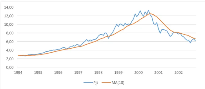
In this section, we will describe the three most common moving averages trading rules. Throughout this section the buy signals are triggered when the indicator is positive and a sell signal when its negative, for all trading rules. In all Figures presented in this section, we use data sample from value-weighted portfolios sorted on book-to-market, decile 1, from the US market. The period of the sample is from January 1994 to December 2002. We will start presenting a popular trading rule that is using the Price-Minus-Moving-Average rule (P-MA), also called price crossover. This indicator compares the current price level Pjt against the Moving Average MAjt,L indicating an upward trend when the MA exceeds the price level, trigging a buy signal. When MA is inferior, it indicates a downward trend triggering a sell signal. This leads to the following formula and further illustrated in Figure 1:

P − MA: @AB7CDEFG#$H+IJKL,M = )

13

Figure 1: Price-minus-moving-average rule

Figure 2: Price-Minus-Moving-Average rule presented by using a window of 10 months. Current price level Pjt presented with a blue line and the MA with 10 months look-back period noted as MA(10) is presented with an orange line. We see the indicator signals to invest in the portfolio mid 1994, and exit mid 2000 when the lines crosses. Also notice the false trading signal mid 1998.

The Moving-Average-Change-of-Direction rule (ΔMA) is triggered in the turning point of a MAjt,L indicating the trend is changing direction. Graphically, turning up from a low point indicates a buy signal and turning down from a peak indicates Sell signal. We can express the rule by the following formula and illustrate it in Figure 2:

∆!": @AB7CDEFG#$∆IJKL,M = !"

#$,&− !"#$+,,&,

Figure 2: Moving-average-change-of-direction rule

Figure 3: Moving-Average-Change-of-Direction rule presented by using a look-back period of 10 months. Current price level Pjt presented with a blue line, the MA with 10 months’ period noted as MA(10) is presented as orange and MA of previous period noted as MAt-1(10) presented as grey. We see the indicator signals to invest in the portfolio mid 1994, and exit mid 2000 as the MA changes direction indicated when the orange and grey line crosses at the bottom and top.

0,00 2,00 4,00 6,00 8,00 10,00 12,00 14,00 1994 1995 1996 1997 1998 1999 2000 2001 2002 Pjt MA(10) 0,00 2,00 4,00 6,00 8,00 10,00 12,00 14,00 1994 1995 1996 1997 1998 1999 2000 2001 2002 Pjt MA(10) MAt-1(10)

14

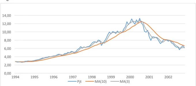
Finally, we have the Double-Crossover Method (DCM). Here it´s used two MA´s: one with a short look-back period and another with a long period. Instead of using the price as in the Price-Minus-Moving-Average rule, the longer MA will replace it, filtered for the noise of the volatility of the frequent return. When the shorter MA crosses above the longer, this indicates an increasing trend that triggers a buy signal, known as a golden cross. And when the shorter MA crosses below the longer, it indicates a declining trend that triggers a sell signal, know as a death cross. We can more formally express the indicator as following:

OP!: @AB7CDEFG#$QRIKL,S,M = !"

#$,T,& − !"#$,&,

where s denotes the MA with the shorter look-back period. On the next page we present the trading rule graphically.

Figure 3: Double-crossover rule

Figure 3:Current price level presented with a blue line, the long MA with 10 months look-back period noted as MA(10) is presented as orange and MA with a 3 months’ period noted as MA(3) as the short is presented as grey. We see the indicator signals to invest in the portfolio mid 1994, and exit mid 2000 as the short MA crosses the longer. Also notice the false trading signal mid 1998.

However, in this thesis we exclusively use the Price-Minus-Moving-Average rule throughout our calculations, which are consistent with the method used by Glabadanidis (2015).

0,00 2,00 4,00 6,00 8,00 10,00 12,00 14,00 1994 1995 1996 1997 1998 1999 2000 2001 2002 Pjt MA(10) MA(3)

15

3.3 Calculating return

Further, we use the indicator to determine if we invest or stay invested in the underlying portfolio when the indicator is positive, and sell the risky portfolio and invest or stay invested in a risk-free portfolio if the indicator is negative. We denote the return of the underlying portfolio as ;_#$. In the case where we are out of the risky portfolio, we invest in a risk-free asset where the risk-free rate of return is denoted as G_U$. We can more formally express the general rule as following:

;_#$,& = ;_G#$, 7V @AB7CDEFG#$+,> 0

U$, YEℎ[G(7\[ ,

where ;#$,& is the return of the active portfolio.

The strategies above were explained in the absence of any transaction costs imposed on the switches. For the rest of the paper and in all of the empirical results quoted, we consider returns after the imposition of a one-way transaction cost of τ at 50 points (0,05%). This is consistent with prior studies like Balduzzi and Lynch (1999), Lynch and Balduzzi (2000) and Han (2006), among others. Regarding the appropriate size of the transaction cost, Balduzzi and Lynch (1999) propose using a value between 1 and 50 basis points. Lynch and Balduzzi (2000) use a midpoint value of 25 basis points. On the side of caution, we use the highest proposed cost. Moreover, in this thesis, we exclusively use the Price-Minus-Moving-Average rule throughout our calculations, which are consistent with the method used by Glabadanidis (2015). Formally, this leads to the following four cases in the post-τ transaction cost returns:

;#$,IJ ;_#$, ;_#$− τ, G_U$, G_U$− τ, 7V )_#$+, > !"_#$+,,& 7V )_#$+, > !"_{#$+,,& 7V )}7V )#$+, < !"#$+,,& #$+,< !"#$+,,& DAB )_#$+- > !" #$+-DAB )_#$+-< !"_#$+- DAB )_#$+- < !" #$+-DAB )_#$+- > !" #$+-,

where ;_#$,IJ is the return of the MA portfolio.

Our extension to the strategy above, we test the moving average switching strategy with short selling the underlying asset and investing the proceeds in G_U$ if )_#$ < !"_#$+,,&. By shorting we will in addition to G_U$ get a payoff equal the difference in the sell price at time t and buy price at time t+1, which is positive given a correct trend prediction. Mathematically this leads to the following four cases:

16 ;_{#$,IJ_} ;_#$, ;_#$− 2τ 2G_U$ − ;_#$ 2G_U$ − ;_#$− 2τ 7V )_#$+,> !"_#$+,,& 7V )_#$+,> !"_#$+,,& 7V )_{7V )}#$+,< !"#$+,,& #$+,< !"#$+,,& DAB )#$+-> !" #$+-DAB )_#$+- < !"_#$+- DAB )_#$+-< !" #$+-DAB )_#$+-> !" #$+-,

where ;_{#$,IJ_} is the return of MAS portfolio.

In the section of results, we will also replicate the MAP portfolio done in Glabadanidis (2015). MAP portfolio is constructed of excess returns as zero-cost portfolios that are long the MA switching strategy and short the underlying portfolio to determine the relative performance of the MA strategy against the buy-and-hold strategy. It denotes the resulting difference between the return of the MA strategy for portfolio j at the end of month t, where ;_#$,IJ is the return on MA portfolio and ;_#$,ab is the return of the passive portfolio. Formally expressed as following:

;_#$,IJH = ;_#$,IJ− ;_#$,ab, c = 1, … , e,

17

4 Theory

4.1 The efficient market hypothesis

In the 1950´s computer applications were in the early phase of analysing the economic market. A natural candidate for the application was to find trends in the behavioural of stock market prices over time. Assuming that stock prices reflect the prospects of the firm, recurrent patterns of peaks and troughs in economic performance ought to show up in those prices. In an early study of serial correlation in stock return, Kendall (1953), in contrary to the assumption found no evidence of predictable patterns in the return of stocks, presenting evidence that prices randomly increased or decreased on any given day regardless of the historical performance. More precise, the price changes are independent of historical movements and identical normal distributed, this led to the theory that stocks follow a random walk, suggesting efficient capital markets.

Moreover, later several economists such as Fama (1965) explored the phenomena and found that price changes occur only when new unpredicted information is presented. These randomly evolving stock prices are a consequence of intelligent investors competing to discover relevant information before the rest of the market becomes aware of it. The movement of the stock price must be a response to the new information. By the definition of new information it can not be predicted, thus, the stock price can not be predicted.

The empirical research in Fama (1970) which led to the efficient market hypothesis (EMH) builds on a large body previous literature, most of which is concerned with general theories and intuitively implications of efficient market models on stock prices rather than empirical evidence. Fama (1970) presents empirical research on whether the movements of stock prices are consistent with the theory of random walk. The study finds extensive evidence in support of the efficient market model, he further distinguishes between the weak, the semi-strong and semi-strong forms of the market efficacy, he also argues that the semi-semi-strong form of the hypothesis should be viewed as the benchmark from which to evaluate deviations in market efficiency. The difference between the forms is what is considered as "all available information". We will briefly describe the market conditions explained in Fama (1970) determining the three states of market efficiency. Firstly, the weak form of the hypothesis defines all information as what can be derived from examining market trading data such as historical prices, trading volumes and short interests. This kind of information is publicly

18

available and relatively easy to obtain and virtually costless. Secondly, the semi-strong form of the hypothesis states that all information publically available regarding the prospects of a firm should already be reflected in the stock prices. In addition to the historical prices it includes fundamental data such as firms' product line, patents held, earning forecast etc. Finally, in the strong form of the hypothesis, it states that all relevant information of the firm is reflected in the stock price, including information that is only available to company insiders. This is the extreme form and might be more of a theory than of practical use. There is no denying inside information has powerful predictive power, as a consequent it is prohibited by law to profit by exploiting their privileged situation, commonly known as inside trading.

According to evidence presented in Fama (1970) markets in the weak form of the hypothesis is not enough to declare the market efficient, but the level of predictability in such markets is too low to be exploited by technical trading strategies due to transaction cost. In general the EMH stated that it is impossible to “beat the market” with technical analysis as markets in all three states of the hypothesis is sufficiently efficient.

Not surprisingly, the hypothesis is not fully accepted and the discussion is still ongoing. Mainly there are three issues that arguably causes the debate to never be settled. While most economists agree that the value of stocks is priced close to their fair value, thus there is needed large portfolios to exploit the minor mispricing to make it worth the effort. The magnitude issue addresses the problem of statistically proving that it was the portfolio manager contribution that led to a minor improvement in performance. Secondly, we have the selection bias issue. The selection of papers and articles observable to the public in biased by preselected failed attempts to find abnormal returns. Presenting a working strategy public would lead the market to adjust the price accordingly to the argument of the EMH. Consequently, there is no way of fairly evaluate the true abilities of portfolio managers to generate winning strategies. Finally, there is the lucky event issue. Some believe that the market could not be efficient because of the frequently published stories of portfolio managers making huge profits over a short period of time. It may be easy to forget that the participating in the stock market is a gamble, not surprisingly there are success stories, however, there are few studies that include how well they do in the next following periods.

While there is academics and practitioners believing that technical analysis is useful despite the EMH, the effectiveness is still being debated. As most economists agree that the values of stocks are prices close to their fair value, thus, there is needed insight to exploit the minor mispricing to make it worth the effort, the easy pickings have probably been picked. This might arguably be the drivers that lead to an efficient market.

19

4.2 Market portfolio Theory 4.2.1 Markowitz

The market portfolio theory describes how to construct a portfolio in order to maximize expected return on a given level of risk defined as standard deviation. This was first presented by Harry Markowitz (1952). The following is the essential estimations for his model.

Expected return and volatility for one single asset

9 G₀ = 1 f G0 g 0 h₀ = 1 f − 1 (G0 − 9[G0]) -g 01, ,

where 9 G₀ is the mean return in asset i and h₀ is the volatility in the return G₀ respectively. T is the sample size.

Further, we can express expected return and volatility in a portfolio

9 G_m = (₀9[G₀] 0 , h_m = (₀(_#h₀h₀n_0# # 0 ,

where 9 Gm is the expected return of the portfolio, 9[G0]is the expected return in asset i and wi

is the weighting of asset i in the portfolio and n_0# is the correlation coefficient between asset i

and j.

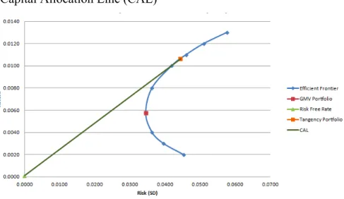
By combining a risky portfolio with risk-free asset one can construct a to capital allocation line (CAL) illustrated in Figure 5. that shows all possible combinations that lead to different expected return given the level of risk along a straight line where the best possible combination is where the CAL tangents the efficient frontier. This line is more formally expressed as:

9 Go = GU+ ho

9 G₀ − G_U h₀ ,

20

where ri is the return of the risky portfolio, rf is the risk-free rate of return and G_o and h_o is the return and standard deviation on the complete portfolio respectively.

We can by these expressions construct optimal weight of assets in a portfolios that offers the highs expected return for a defined level of risk, thru diversification. Displaying graphically all the combinations of optimal portfolios we get a hyperbola. The lowest possible risk along the hyperbola shows the global minimum variance portfolio (GMV), which is obtained by minimizing the expression for portfolio volatility. All portfolio combinations above the point of GMV on the hyperbola is located on what Markowitz refer to as the efficient frontier. Beneath the GMV is not defined as efficient as one can choose a different combination of assets in a portfolio that produces a higher expected return with the same risk.

Figure 4: The Capital Allocation Line (CAL)

Figure 4: The hyperbola marked as blue illustrates all outer points of possible combinations of risky portfolios. Above the GMV portfolio is defined as the efficient frontier. The CAL marked as green illustrates the the possible expected returns by combinations of risky- and risk free assets (this case the risk free rate of return is 0).

21

4.2.2 Sharpe ratio

Building on the market portfolio theory of Markowitz (1952), the Sharpe ratio was developed and named after William Sharpe for evaluating assets (Sharpe (1966)). The ratio is used to calculate the risk-adjusted return and is still the industry standard, which we also use in this thesis to evaluate portfolio performance. We can express the ratio as following:

3ℎDGp GDE7F = 9 G0 − GU h_0+U ,

where Let (9 G₀ − G_U) be the return on a risky asset in the excess of the risk-free rate of return and denote h_0+U as the respective volatility.

4.3 Alpha as performance measure

We will in this section briefly describe the portfolio performance measure alpha and theory behind the models used in our thesis to estimate it. The asset pricing models use market factors to estimate the expected rate of return in a certain portfolio through regression at a given time. The alpha is the intercept of the regression indicating whether the the actual return is higher or lower compared to what’s expected given the current circumstances. Alpha is a key measure for performance in modern portfolio theory, due to it’s applicability to any portfolio, and are relatively simple to interpret. It is suitable for comparisons since it uses a percentage measures of the deviation between the actual return and the expected risk-adjusted return of an equity security.

4.3.1 The capital asset pricing model

The Capital Asset Pricing Model (CAPM) was developed in the 1960’s by Sharpe (1964), Traynor (1962), Lintner (1965) and Mossin (1966), and still remains a popular and commonly used theory of determining the required rate of returns of securities. William Sharpe and John Lintner first introduced the model by building on the previous work of Harry Markowitz, adding several assumptions, such as the possibility of lending and borrowing at the risk-free rate, that capital markets is in an equilibrium state, that all investors have access to the same investment opportunities and that all investors have an identical investment horizon.

22

The model builds on the modern portfolio theory by Markowitz, which assumes that investors hold fully diversified portfolios only containing systematic risk. Following the assumptions, the model compensates investors only for undiversifiable risk and the time value of money, not the total risk. In the model, beta represents the systematic risk of an asset and is estimated by regressing historical excess returns of an asset on the average market premium for the same period. The resulting regression coefficient u_#,v is according to the CAPM representing the systematic risk and is a measure of the asset´s risk in relation to the market. Investors then expects to be compensated with a risk premium which is a ratio between the future expected excess return on the market and beta. More formally u_#,v is expressed as follows:

u_#,v =PFw(G#, Gv) h_v- ,

where PFw(G_#, G_v) is the covariance of return between the asset and the market and h_v-_{, the}

market variance. The full model determining the required rate of return can be expressed as follows:

9[G#] − GU= u#,v 9 Gv8$ − GU ,

where 9[G_#] is the expected rate of return on an asset, G_U represents the time value of money and 9[G_v8$] the expected return on the market.

Despite the popular use of the capital asset model research have identified several deficiencies, one of the most prominent is the so-called size or small-firm effect, originally documented by Banz (1981). Empirical research shows that small firms systematically generate higher abnormal returns estimated by CAPM compared to the bigger capitalized firms. While the smaller-sized portfolios have generally higher volatility, the performance is still better. There have been many researchers that have tried to explain the abnormality without an exclusive answer. However, the phenomena have been consistent in the past, including the data in our sample.

Fama French (1992) showed that a powerful predictor of returns across securities is the ratio of the book value of the firm’s equity to the market value of equity. Fama and French stratified firms into 10 deciles according to book-to-market ratios and examined the average monthly rate of return of each of the 10 groups. The decile with the highest book-to-market ratio had a substantial higher abnormal returns compared with the lowest ratio decile. The dramatic dependence of returns on book- to-market ratio has been shown to be independent of

23

beta in CAPM. This suggest either that high book-to-market ratio firms are relatively underpriced, or that the book-to-market ratio is serving as a proxy for a risk factor that affects equilibrium expected returns.

4.3.2 Fama-French 3-factor model

To address the size and book-to-market anomalies, Fame-French (1993) presents a multidimensional model that extends CAPM with two new variables, SMB (small minus big) and HML (high minus low) to address the anomalies respectively. The SMB factor accounts for the spread in returns between firms with high and low market capitalization and the HML factor accounts for the spread in returns between value and growth stocks.

The factors are constructed by using 6 value-weighted portfolios formed on size and book-to-market. The size factor (SMB) is the average return on the three small portfolios minus the average return on the three big portfolios. The book-to-market factor (HML) is the average return on the two value portfolios minus the average return on the two growth portfolios. Let 9[GTvx,$] be the expected size factor and 9[Gyvz,$] be the expected book-to-market factor. The

model can be expressed as follows:

9[G#] − GU = u#,v9[Gv8$− GU] + u#,T9[GTvx] + u#,y9[Gyvz],

where beta denoted s and h are the coefficients for size and book-to-market factors respectively.

4.3.3 Fama-French-Carhart 4-factor model

The Fama-French-Carhart 4-factor model is an extension of the Fama-French 3-factor model including a momentum anomaly first documented in Jegadeesh and Titman (1993). Jegadeesh and Titman uncovered a tendency for good or bad performance of stocks to persist over several months. They conclude that while the performance of individual stocks is highly unpredictable, portfolios of the best-performing stocks in the recent past appear to outperform other stocks. Carhart (1997) presented evidence that the 4-factor model incorporating the momentum anomaly was able to account for a sizable time series variation and on average price assets more accurate than the CAPM and the 3-factor model before.

The momentum factor, UMD (Up Minus Down), is the average return on the two robust operating profitability portfolios minus the average return on the two weak operating

24

profitability portfolios. Let 9 G_{v| be the expected momentum factor, the model can be expressed as follows:

9[G_#] − G_U = u_#,v9 G_v8$− G_U + u_#,T9 G_Tvx + u_#,y9 G_yvz + u_#,{9 G_{v| , where beta denoted u is the coefficient for momentum factor.

4.3.4 Regression models

In our thesis we perform multiple OLS regression analysis on the portfolio returns using the capital asset pricing model (CAPM), 3 factor model (FF3F) and Fama-French-Carhart-4 factor (FFC4F) model to estimate the excess return, alpha (}). Using the same notations as mention in the sections above we can express the regressions as follows:

The capital asset pricing model

G_# − G_U = }_#+ u_#,v(G_v8$− G_U) + ~_#, c = 1, … , e, Fama-French-3 factor model

G_#− G_U = }_# + u_#,v(G_v8$ − G_U) + u_#,TG_Tvx+ u_#,yG_yvz + ~_#, c = 1, … , e, Fama-French-Carhart-4 factor model

G_# − G_U= }_#+ u_#,v(G_v8$− G_U) + u_#,TG_Tvx+ u_#,yG_yvz+ u_#,{G_{v|+ ~_#, c = 1, … , e, where ~_# is denoted as the error term. In the regression we test if the estimated alphas are significant different from zero. Formally expressed as following:

₂: }_# = 0, _J: }_# ≠ 0

25

5 Testing

In this section, we will describe how we test our data empirically. We test if the implemented active strategies can achieve a higher risk-adjusted return measured by the Sharpe ratio, than by simply applying the passive BH strategy. Further, we test statistically if there is a significantly difference in the estimated alphas between the active and passive strategies. If we can identify a significantly higher Sharpe ratio or a significant higher alpha, it implies that the active strategies have the ability to outperform the passive BH strategy.

5.1 Sharpe ratio

For testing the Sharpe ratio, we use the Jobson and Korkie (1981) test with the Memmel (2003) correction. Specifically, given two portfolios, passive and active denoted 3;_m and 3;_J respectively as their estimated Sharpe ratios. We test the null hypothesis against our alternative hypothesis as following:

₂: 3;_m ≥ 3;_J, _J: 3;_m < 3;_J,

Let ρ be the correlation coefficient over a sample of size T. The test statistic is obtained by

Ç = 3;m− 3;J

1

f [2 1 − n- + 12 3;m-+ 3;J-− 23;m3;Jn- ]

,

which is asymptotically distributed as a standard normal. We reject H0 if the p-value is below a significance level of 0,05.

26

5.2 Alpha

We implement a statistical test in order to determine if the estimated alphas conducted in our active portfolios is superior over the passive. We test if there are significant differences between the portfolios where the estimated alphas appear to be higher with the active strategies compared with their passive counterpart. We used a two-sample t-test. Let α_Ñ be the alpha estimated from the active portfolio and α_Ö be the respective estimated alpha of the passive BH portfolio. We test the null hypothesis against our alternative hypothesis as following:

2: αÖ≥ αÑ, J: αÖ< αÑ,

We calculated the test statistic1 as following.

E = αÖ− αÑ σ_Ö-_{+ σ} Ñ

,

where h_J and h_m is the standard error of the estimation of alpha from the active and passive portfolios respectively. We reject ₂if the p-value is below a significance level of 0,05.

1. Since our data sample is relatively large, the t-distribution will be close to a standard normal, we will therefore derive the p-value with the assumption of normal distribution.

27

6 Data

We use monthly value-weighted returns of sets of 10 US portfolios as well as sets of 10 Norwegian portfolios sorted by size, book-to-market and momentum. US portfolios is constructed by including all NYSE, AMEX, and NASDAQ stocks for which we have market equity data for. The Norwegian portfolios are constructed by using stocks from the OSE. Value weighted portfolios are weighted within the relevant index based on a calculation of each stock's absolute and relative value as compared to other stocks within the index. The index is continually rebalanced, the portfolios are updated as prices and company fundamentals change. We use the return on the 30-day US Treasury Bill as a proxy for the risk-free rates in the US market. A 30-days estimated from forward-looking government securities fromNorwegian Interbank Offered Rate (NIBOR) as a proxy for the risk-free rate of return for the Norwegian market.

The data are readily available from Ken French Data Library1 for US data and Bernt Arne Ødegaard2 data library for Norwegian data. The sample period starts in December 1957 and ends in December 2011 for US data and starts in January 1980 and ends in December 2015 for Norwegian data. However, because of moving averages uses historical data determined by the look-back period, the results are presented from January 1960 for the US data and February 1982 for the Norwegian data. Next page in Table 1 we have made a descriptive summary statistic for all portfolios used in our thesis.

1. http://mba.tuck.dartmouth.edu/pages/faculty/ken.french/data_library.html 2. http://finance.bi.no/~bernt/financial_data/ose_asset_pricing_data/index.html

28

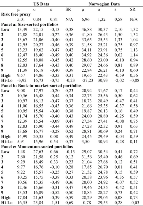
Table 1: Descriptive statistics

US Data Norwegian Data

Norwegian Data

µ σ s SR µ σ s SR

Risk free proxy

5,01 0,84 0,81 N/A 6,96 1,32 0,58 N/A

Panel a: Size-sorted portfolios

Low 13,49 22,15 -0,13 0,38 46,88 30,37 2,10 1,32 2 12,88 22,01 -0,22 0,36 41,80 26,43 1,50 1,32 3 13,67 21,06 -0,40 0,41 33,65 25,53 1,33 1,04 4 12,95 20,27 -0,46 0,39 31,58 25,21 0,75 0,97 5 13,23 19,62 -0,47 0,42 34,11 23,91 0,75 1,13 6 12,47 18,40 -0,49 0,40 34,92 24,36 0,62 1,14 7 12,55 18,08 -0,45 0,42 28,60 23,00 -0,10 0,94 8 12,03 17,64 -0,43 0,40 29,07 24,66 0,81 0,89 9 11,39 16,18 -0,40 0,39 22,84 26,21 -0,10 0,60 High 9,57 14,86 -0,33 0,31 19,65 22,43 -0,59 0,56 Hi-Lo -3,92 16,73 -0,75 -0,23 -27,23 30,93 -2,02 -0,88 Panel b: Book-to-market-sorted portfolios

Low 9,08 17,97 -0,20 0,23 20,94 31,67 0,17 0,44 2 10,56 16,48 -0,44 0,34 22,75 25,56 0,50 0,62 3 10,97 16,13 -0,47 0,37 18,73 28,49 -0,47 0,41 4 11,00 16,55 -0,43 0,36 21,66 25,35 -0,37 0,58 5 10,95 15,54 -0,40 0,38 19,87 26,13 0,16 0,49 6 11,74 15,70 -0,40 0,43 24,00 28,80 -0,25 0,59 7 12,39 15,54 -0,09 0,47 27,54 27,41 -0,08 0,75 8 12,83 15,90 -0,44 0,49 27,28 32,32 0,91 0,63 9 13,68 16,77 -0,28 0,52 28,81 30,69 0,24 0,71 High 14,99 20,35 0,08 0,49 24,45 29,49 -0,04 0,59 Hi-Lo 5,91 15,96 0,54 0,37 3,50 30,94 -0,28 0,11 Panel c: Momentum-sorted portfolios

Low 1,48 27,63 0,66 -0,13 29,07 30,54 0,41 0,72 2 7,60 21,58 0,25 0,12 31,56 35,40 0,46 0,69 3 9,29 18,49 0,33 0,23 21,04 27,68 0,12 0,51 4 9,77 16,76 -0,10 0,28 17,85 26,70 0,01 0,41 5 9,22 15,57 -0,25 0,27 21,52 24,78 0,15 0,59 6 10,25 15,75 -0,38 0,33 20,58 23,96 -0,35 0,57 7 10,56 15,35 -0,49 0,36 20,00 24,92 -0,07 0,52 8 12,46 15,66 -0,31 0,47 19,46 24,35 -0,42 0,51 9 13,53 16,89 -0,52 0,50 18,85 28,27 0,73 0,42 High 17,84 21,63 -0,39 0,59 28,29 29,05 0,08 0,73 Hi-Lo 16,35 23,84 -1,51 0,69 -0,78 29,53 0,28 -0,03

Table 1: This table reports the summary statistics for the US and Norwegian data sample. The sample period covers January 1960–December 2011 for the US and February 1980-December 2015 for the Norwegian with value-weighted portfolio returns. All data is presented annual in percentage. µ is the average return, σ is the standard deviation of returns, s is the skewness, and SR is the Sharpe ratio.

29

7 Results

In this section, we present our results conducted by the tests described in previous sections. First, we will present replicated results published by Glabadanidis in 2015 his paper “Market timing with moving averages”. Further, we will present the simple moving average switching strategy with and without exercising a short sale on the underlying portfolio. We used the more common 10 months look-back period to for both active strategies in the US and Norwegian stock market. This is consistent with former studies including Brock et al (1992), Siegel (2002, Chapter 17), and Faber (2007) where the authors acknowledge that 10-month (200-day) MA rule is the most popular trading rule among practitioners. We have also tested look-back periods of 8 and 12 months as a robustness check. On the basis of Carhart (1997) presenting evidence of the Fama-French-Carhart 4-Factor model´s superior ability in explaining time series variation, will only present alphas estimated by this model. However, the estimated alphas from Fama-French 3-Factor and CAPM is readily available in the Appendix.

7.1 Replicating Glabadanidis

We first implemented the MA switching strategy replicating the method used in Glabadanidis (2015). The data sample is from the US market in the period January 1960 to December 2011, and using a look-back period of 24 months. At first, we were unable to replicate his results, but after extensive work we found a method using a look-ahead-bias that gave us similar results, this is possibly the same bias as in his paper. The bias is a result of using the price level from the current period (t) that has not been realized to calculate the moving average. By using the same notations as earlier we can more formally express it as following:

;_#$,& = ;_G#$, 7V )#$ > !"#$,&

U$, YEℎ[G(7\[

After implementing this bias, we arrived at the similar results presented in Table 2. In the results from the biased MA strategy, there was exclusively higher average return compared with BH strategy. This combined with lower standard deviation resulted in significant higher Sharpe ratios for all deciles in all portfolios. There was also identified high positive significant alphas estimated by the Fama-French-Carhart 4-factor (FFC4F) model for all tested. All measures providing strong evidence of superior performance over the passive strategy.

However, when correcting for the bias, the performance of MA strategy was greatly reduced. In Table 3 we can see that the results of the general annual average return were lower

30

with the MA strategy than BH strategy, in average 1-2% lower, with the exception of portfolios sorted on momentum, decile 1. This is also reflected in the MAP portfolios where the average returns are negative. Note that even when the standard deviation overall is lower with MA strategy, the Sharpe ratios does not exceed BH. The implemented Sharpe test could neither identify any significant difference.

Looking at the MA portfolio alphas estimated by FFC4F regression model we observe that most of the alphas is negative with the exception of one portfolio sorted on momentum, decile 10. Moreover, the significant alphas are all highly negative, ranging between 2-6%. This suggests that the MA portfolios has lower risk adjusted return than expected. Further evidence of inferior performance can be observed by comparing the skewness of BH and MA strategy. Even though the vast majority of the underlying BH exhibits negative skewness, it may look like the distribution of returns in MA strategy is even more negatively skewed, indicating poorer performance of the MA strategy.

After the correction of the bias we were left with no evidence of superior performance of MA strategy over the passive BH strategy. Presenting the data graphical in Figure 6 the differences becomes compelling.

31

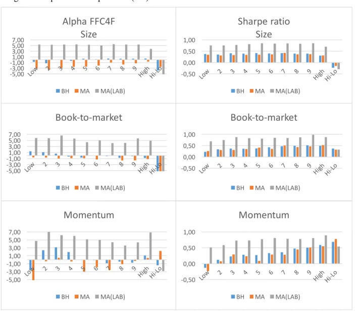
Figure 5: Alpha and Sharpe ratios (US)

Figure 5: Graphically illustrated alphas and Sharpe ratios in the right and left column respectively. Data is presented in the replicated data of Glabadanidis in table 2 and 3. Passive strategy buy and hold (BH) presented as blue, active strategy moving average switching strategy (MA) presented as orange, moving average with look-ahead-bias (MA LAB) presented as grey

-5,00 -3,00 -1,001,00 3,00 5,00 7,00

Alpha FFC4F

Size

Book-to-market

Momentum

Sharpe ratio

Size

Book-to-market

Momentum

32

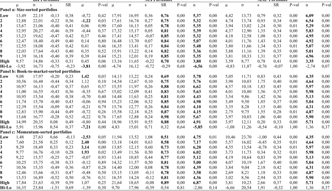
Table 2: This table reports the summary statistics for the respective buy-and-hold (BH) portfolio returns, the replicated moving average (MAR) switching strategy portfolio returns and the excess return of MAD over BH (MAP). The sample period covers January 1960–December 2011 with value-weighted portfolio returns. μ is the annualized average return, σ is annualized standard deviation of returns, s is the annualized skewness, and SR is the annualized Sharpe ratio, ! is the alpha from Fama-French-Carhart 4-factor model. The length of the look-back period is 24 months. For the Sharpe ratio of the MA strategy, we test the hypothesis "0: %&'" ≥ %&)*(%). For each alpha, we test the hypothesis H0 : α = 0. Bold text indicate values that are statistically significant at the 5% level

µ σ s SR ! P-val µ σ s SR P-val α P-val µ σ s SR P-val α P-val

Panel a: Size-sorted portfolios

Low 13,49 22,15 -0,13 0,38 -0,72 0,42 17,91 16,95 0,36 0,76 0,00 5,37 0,00 4,42 13,73 0,79 0,32 0,00 6,09 0,00 2 12,88 22,01 -0,22 0,36 -1,22 0,03 17,61 16,74 0,27 0,75 0,00 5,32 0,00 4,74 13,74 0,93 0,34 0,00 6,54 0,00 3 13,67 21,06 -0,40 0,41 0,06 0,90 17,60 16,13 0,05 0,78 0,00 5,35 0,00 3,94 13,02 1,24 0,30 0,01 5,29 0,00 4 12,95 20,27 -0,46 0,39 -0,44 0,37 17,32 15,17 0,05 0,81 0,00 5,39 0,00 4,37 12,90 1,35 0,34 0,00 5,83 0,00 5 13,23 19,62 -0,47 0,42 0,37 0,46 17,41 14,57 -0,07 0,85 0,00 5,32 0,00 4,18 12,58 1,08 0,33 0,00 4,95 0,00 6 12,47 18,40 -0,49 0,40 0,14 0,80 16,48 13,70 0,07 0,84 0,00 5,07 0,00 4,01 11,76 1,43 0,34 0,00 4,92 0,00 7 12,55 18,08 -0,45 0,42 0,41 0,46 16,35 13,41 0,17 0,84 0,00 5,48 0,00 3,80 11,66 1,34 0,33 0,01 5,07 0,00 8 12,03 17,64 -0,43 0,40 0,35 0,52 15,91 13,22 0,14 0,82 0,00 5,36 0,00 3,88 11,16 1,39 0,35 0,00 5,01 0,00 9 11,39 16,18 -0,40 0,39 0,39 0,44 15,21 12,01 0,19 0,85 0,00 5,35 0,00 3,81 10,33 1,31 0,37 0,00 4,96 0,00 High 9,57 14,86 -0,33 0,31 0,45 0,06 13,16 11,65 -0,22 0,70 0,00 3,80 0,00 3,59 8,77 0,78 0,41 0,00 3,35 0,00 Hi-Lo -3,92 16,73 -0,75 -0,23 -3,81 0,00 -4,74 16,12 -0,72 -0,29 0,68 -6,56 0,00 -0,83 11,87 -0,76 -0,07 1,00 -2,74 0,07 Panel b: Book-to-market-sorted portfolios

Low 9,08 17,97 -0,20 0,23 1,42 0,03 14,13 13,22 0,24 0,69 0,00 5,78 0,00 5,05 11,71 0,83 0,43 0,00 4,35 0,00 2 10,56 16,48 -0,44 0,34 1,12 0,10 14,54 12,67 0,10 0,75 0,00 5,76 0,00 3,98 10,03 1,75 0,40 0,00 4,64 0,00 3 10,97 16,13 -0,47 0,37 0,65 0,37 15,55 11,97 0,26 0,88 0,00 6,62 0,00 4,57 10,18 1,83 0,45 0,00 5,97 0,00 4 11,00 16,55 -0,43 0,36 -0,35 0,67 15,02 12,09 0,41 0,83 0,00 5,63 0,00 4,01 10,80 1,56 0,37 0,00 5,98 0,00 5 10,95 15,54 -0,40 0,38 -0,70 0,40 14,48 11,63 0,25 0,81 0,00 4,43 0,00 3,54 9,86 1,42 0,36 0,00 5,13 0,00 6 11,74 15,70 -0,40 0,43 -0,06 0,94 15,23 12,06 0,32 0,85 0,00 4,98 0,00 3,49 9,50 1,85 0,37 0,00 5,04 0,00 7 12,39 15,54 -0,09 0,47 -0,21 0,79 15,74 12,77 0,26 0,84 0,00 4,10 0,00 3,35 8,28 1,15 0,40 0,00 4,31 0,00 8 12,83 15,90 -0,44 0,49 -0,72 0,26 15,58 12,18 0,25 0,87 0,00 4,15 0,00 2,75 9,75 1,55 0,28 0,01 4,87 0,00 9 13,68 16,77 -0,28 0,52 -0,22 0,76 17,65 12,88 0,24 0,98 0,00 5,67 0,00 3,97 10,03 1,06 0,40 0,00 5,90 0,00 High 14,99 20,35 0,08 0,49 -0,80 0,44 18,96 15,91 0,55 0,88 0,00 4,91 0,00 3,97 12,11 0,20 0,33 0,00 5,71 0,00 Hi-Lo 5,91 15,96 0,54 0,37 -7,21 0,00 4,83 15,01 0,71 0,32 0,64 -5,85 0,00 -1,08 11,26 -0,54 -0,10 1,00 1,36 0,37 Panel c: Momentum-sorted portfolios

Low 1,48 27,63 0,66 -0,13 -2,53 0,05 11,94 13,52 1,08 0,51 0,00 4,75 0,01 10,46 23,70 -1,00 0,44 0,00 4,35 0,00 2 7,60 21,58 0,25 0,12 2,40 0,00 13,18 14,01 0,63 0,58 0,00 7,17 0,00 5,57 16,02 -0,45 0,35 0,01 4,64 0,00 3 9,29 18,49 0,33 0,23 3,14 0,00 13,85 12,15 0,60 0,73 0,00 6,20 0,00 4,55 13,54 -0,78 0,34 0,01 5,97 0,00 4 9,77 16,76 -0,10 0,28 1,93 0,02 13,49 11,56 0,50 0,73 0,00 6,02 0,00 3,73 11,73 0,34 0,32 0,01 5,98 0,00 5 9,22 15,57 -0,25 0,27 -0,07 0,93 13,41 10,85 0,44 0,77 0,00 5,12 0,00 4,19 10,64 0,83 0,39 0,00 5,13 0,00 6 10,25 15,75 -0,38 0,33 -0,12 0,89 14,32 11,57 0,50 0,81 0,00 5,00 0,00 4,07 10,19 1,67 0,40 0,00 5,04 0,00 7 10,56 15,35 -0,49 0,36 -0,87 0,28 14,40 12,00 0,08 0,78 0,00 4,39 0,00 3,84 9,04 2,18 0,42 0,00 4,31 0,00 8 12,46 15,66 -0,31 0,47 -0,48 0,50 15,15 13,05 -0,11 0,78 0,00 3,58 0,00 2,69 8,21 1,18 0,33 0,00 4,87 0,00 9 13,53 16,89 -0,52 0,50 -0,76 0,31 16,55 14,24 -0,12 0,81 0,00 4,36 0,00 3,02 8,56 2,94 0,35 0,00 5,90 0,00 High 17,84 21,63 -0,39 0,59 1,07 0,25 21,64 18,65 -0,08 0,89 0,00 6,87 0,00 3,81 10,23 2,66 0,37 0,00 5,71 0,00 Hi-Lo 16,35 23,84 -1,51 0,69 -1,39 0,30 9,70 17,96 -0,39 0,54 0,81 -2,86 0,14 -6,66 20,54 1,91 -0,32 1,00 1,36 0,37

33

This table reports the summary statistics for the respective buy-and-hold (BH) portfolio returns, the moving average (MA) switching strategy portfolio returns and the excess return of MA over BH (MAP). The sample period covers January 1960–December 2011 with value-weighted portfolio returns. μ is the annualized average return, σ is annualized standard deviation of returns, s is the annualized skewness, and SR is the annualized Sharpe ratio, ! is the alpha from Fama-French-Carhart 4-factor model. The length of look-back period is 24 months. For the Sharpe ratio of the MA strategy, we test the hypothesis "0: %&'" ≥ %&)*(%).

For each alpha, we test the hypothesis H0 : α = 0. Bold text indicate values that are statistically significant at the 5% level.

µ σ s SR ! P-val µ σ s SR P-val α P-val µ σ s SR P-val α P-val

Panel a: Size-sorted portfolios

Low 13,49 22,15 -0,13 0,38 -0,72 0,42 11,18 17,59 -0,26 0,35 0,60 -3,13 0,04 -2,31 13,54 -0,62 -0,17 1,00 -2,41 0,08 2 12,88 22,01 -0,22 0,36 -1,22 0,03 10,62 17,91 -0,34 0,31 0,65 -3,39 0,01 -2,25 12,94 -0,54 -0,17 1,00 -2,17 0,10 3 13,67 21,06 -0,40 0,41 0,06 0,90 10,69 17,30 -0,55 0,33 0,77 -2,91 0,03 -2,97 12,14 -0,36 -0,24 1,00 -2,97 0,02 4 12,95 20,27 -0,46 0,39 -0,44 0,37 10,54 16,16 -0,54 0,34 0,66 -2,52 0,05 -2,41 12,36 0,03 -0,19 1,00 -2,08 0,10 5 13,23 19,62 -0,47 0,42 0,37 0,46 10,49 15,77 -0,72 0,35 0,73 -2,47 0,05 -2,73 11,79 -0,41 -0,23 1,00 -2,84 0,02 6 12,47 18,40 -0,49 0,40 0,14 0,80 10,34 14,83 -0,68 0,36 0,65 -2,05 0,09 -2,13 11,00 -0,21 -0,19 1,00 -2,20 0,06 7 12,55 18,08 -0,45 0,42 0,41 0,46 11,11 14,42 -0,57 0,42 0,48 -1,01 0,39 -1,45 10,98 -0,05 -0,13 1,00 -1,42 0,23 8 12,03 17,64 -0,43 0,40 0,35 0,52 10,11 14,00 -0,49 0,36 0,61 -1,68 0,14 -1,92 10,83 0,02 -0,18 1,00 -2,04 0,08 9 11,39 16,18 -0,40 0,39 0,39 0,44 9,76 12,76 -0,48 0,37 0,57 -1,24 0,25 -1,63 10,02 -0,04 -0,16 1,00 -1,63 0,13 High 9,57 14,86 -0,33 0,31 0,45 0,06 8,81 11,97 -0,36 0,32 0,46 -0,68 0,49 -0,76 8,89 0,03 -0,09 0,99 -1,12 0,25 Hi-Lo -3,92 16,73 -0,75 -0,23 -3,81 0,00 -2,37 15,61 -0,70 -0,15 0,27 -2,53 0,11 1,55 11,88 0,68 0,13 0,02 1,28 0,40 Panel b: Book-to-market-sorted portfolios

Low 9,08 17,97 -0,20 0,23 1,42 0,03 8,60 13,86 -0,32 0,26 0,40 -0,61 0,62 -0,48 11,44 -0,13 -0,04 0,96 -2,04 0,09 2 10,56 16,48 -0,44 0,34 1,12 0,10 9,12 13,49 -0,53 0,30 0,61 -0,68 0,56 -1,44 9,50 0,00 -0,15 1,00 -1,80 0,10 3 10,97 16,13 -0,47 0,37 0,65 0,37 9,00 13,07 -0,67 0,30 0,71 -0,99 0,41 -1,97 9,50 -0,20 -0,21 1,00 -1,64 0,12 4 11,00 16,55 -0,43 0,36 -0,35 0,67 9,62 13,34 -0,47 0,35 0,55 -0,89 0,47 -1,38 9,84 0,16 -0,14 1,00 -0,54 0,62 5 10,95 15,54 -0,40 0,38 -0,70 0,40 10,16 12,54 -0,60 0,41 0,40 -0,87 0,47 -0,79 9,22 -0,34 -0,09 1,00 -0,18 0,86 6 11,74 15,70 -0,40 0,43 -0,06 0,94 9,63 12,89 -0,52 0,36 0,73 -1,27 0,28 -2,11 9,12 -0,45 -0,23 1,00 -1,21 0,25 7 12,39 15,54 -0,09 0,47 -0,21 0,79 11,49 12,72 -0,12 0,51 0,38 -0,03 0,98 -0,90 8,95 -0,80 -0,10 1,00 0,18 0,86 8 12,83 15,90 -0,44 0,49 -0,72 0,26 10,68 13,10 -0,24 0,43 0,70 -1,64 0,15 -2,15 9,17 0,44 -0,23 1,00 -0,92 0,39 9 13,68 16,77 -0,28 0,52 -0,22 0,76 11,34 13,69 -0,36 0,46 0,68 -1,58 0,19 -2,33 9,83 -0,74 -0,24 1,00 -1,36 0,22 High 14,99 20,35 0,08 0,49 -0,80 0,44 13,26 15,85 -0,16 0,52 0,40 -1,18 0,43 -1,73 12,85 -1,51 -0,13 1,00 -0,38 0,79 Hi-Lo 5,91 15,96 0,54 0,37 -7,21 0,00 4,66 14,54 0,20 0,32 0,64 -5,56 0,00 -1,25 12,04 -0,73 -0,10 1,00 1,65 0,29 Panel c: Momentum-sorted portfolios

Low 1,48 27,63 0,66 -0,13 -2,53 0,05 1,94 13,04 -0,50 -0,23 0,73 -6,76 0,00 0,46 24,36 -0,97 0,02 0,06 -4,24 0,02 2 7,60 21,58 0,25 0,12 2,40 0,00 6,03 13,79 0,05 0,07 0,62 -0,39 0,81 -1,57 16,65 -0,71 -0,09 0,96 -2,78 0,07 3 9,29 18,49 0,33 0,23 3,14 0,00 8,52 11,97 0,30 0,29 0,34 0,46 0,73 -0,77 14,11 -0,88 -0,05 0,99 -2,68 0,04 4 9,77 16,76 -0,10 0,28 1,93 0,02 7,89 12,03 -0,14 0,24 0,63 -0,43 0,73 -1,88 11,73 -0,29 -0,16 1,00 -2,35 0,05 5 9,22 15,57 -0,25 0,27 -0,07 0,93 6,05 11,94 -0,66 0,09 0,93 -3,01 0,01 -3,17 10,05 -0,72 -0,32 1,00 -2,94 0,01 6 10,25 15,75 -0,38 0,33 -0,12 0,89 8,69 12,71 -0,54 0,29 0,64 -1,83 0,12 -1,57 9,40 -0,19 -0,17 1,00 -1,71 0,10 7 10,56 15,35 -0,49 0,36 -0,87 0,28 8,72 13,09 -0,61 0,28 0,77 -2,57 0,03 -1,84 8,19 -0,22 -0,22 1,00 -1,69 0,08 8 12,46 15,66 -0,31 0,47 -0,48 0,50 11,10 13,67 -0,35 0,45 0,62 -1,12 0,31 -1,36 7,73 -0,58 -0,18 1,00 -0,63 0,49 9 13,53 16,89 -0,52 0,50 -0,76 0,31 12,70 14,98 -0,48 0,51 0,46 -0,28 0,82 -0,82 7,92 0,46 -0,10 1,00 0,49 0,62 High 17,84 21,63 -0,39 0,59 1,07 0,25 15,94 19,90 -0,39 0,55 0,71 0,46 0,75 -1,90 8,70 -0,82 -0,22 1,00 -0,61 0,57 Hi-Lo 16,35 23,84 -1,51 0,69 -1,39 0,30 14,00 17,96 -0,22 0,78 0,30 2,24 0,24 -2,35 22,01 1,38 -0,11 1,00 3,63 0,06

34 7.2 US portfolios

As we were unable to identify evidence of superior performance by applying the MA switching strategy with a look-back period of 24 months, we investigated further with the more widely used period of 10 months. Addition to this, we also implement another MA switching strategy combined with shorting the underlying portfolio (MAS).

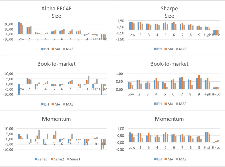
Looking at Table 4, we observe in general that the average returns of MA portfolios compared to BH are substantially lower. However, the average return was improved compared to the strategy with a look-back period of 24 months presented in Table 3. The exception is the lower deciles in momentum where the average returns from MA strategy actually exceed BH. Note that the standard deviation is remarkably lower for all the portfolios, and at first glance the Sharpe ratios in MA seems to exceed the BH portfolios in several deciles. However, we are not able to identify any statistically significant improvement in Sharpe ratios between the portfolios.

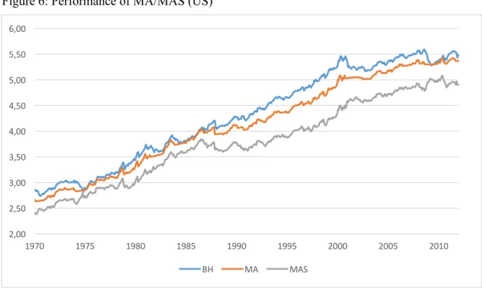
Figure 6: Performance of MA/MAS (US)

Over to the MAS portfolios, the alphas conducted tends to be amplified in the same direction

Figure 6: The performance of US portfolio sorted on momentum, decile 10. The sample period is from January 1970 to December 2011. The price level of the portfolio from passive strategy BH is marked as blue, MA as orange and MAS with grey. The graph is presented in monthly intervals, with log of the price level on the Y axis and the respective time period on the x axis. We see that the passive strategy dominates both active strategies in the figure.

2,00 2,50 3,00 3,50 4,00 4,50 5,00 5,50 6,00 1970 1975 1980 1985 1990 1995 2000 2005 2010 BH MA MAS

35

The MAS strategy tend to amplify the performance in the same direction as we observe when using the MA strategy, which is expected due to the nature of the strategy. MAS is performing poorer in general when MA strategy i