Theses Thesis/Dissertation Collections
5-1-2012
Perceptually optimized real-time computer
graphics
Jeffrey Smith
Follow this and additional works at:http://scholarworks.rit.edu/theses
This Thesis is brought to you for free and open access by the Thesis/Dissertation Collections at RIT Scholar Works. It has been accepted for inclusion in Theses by an authorized administrator of RIT Scholar Works. For more information, please [email protected].
Recommended Citation
Real-Time Computer Graphics
by
Jeffrey D. Smith
A Thesis Submitted in Partial Fulfillment of the Requirements for the Degree of Master of Science
in Computer Engineering
Supervised by
Assistant Professor Dr. Reynold Bailey Department of Computer Science Kate Gleason College of Engineering
Rochester Institute of Technology Rochester, New York
May 2012
Approved by:
Dr. Reynold Bailey, Assistant Professor
Thesis Advisor, Department of Computer Science
Dr. Roy Melton, Senior Lecturer
Committee Member, Department of Computer Engineering
Dr. Muhammad Shaaban, Associate Professor
Rochester Institute of Technology Kate Gleason College of Engineering
Title:
Perceptually Optimized Real-Time Computer Graphics
I, Jeffrey D. Smith, hereby grant permission to the Wallace Memorial Library to reproduce my thesis in whole or part.
Jeffrey D. Smith
Acknowledgments
Abstract
Perceptually Optimized Real-Time Computer GraphicsJeffrey D. Smith
Supervising Professor: Dr. Reynold Bailey
Perceptual optimization, the application of human visual perception mod-els to remove imperceptible components in a graphics system, has been proven effective in achieving significant computational speedup. Previous implementations of this technique have focused on spatial level of detail reduction, which typically results in noticeable degradation of image qual-ity. This thesis introduces refresh rate modulation (RRM), a novel percep-tual optimization technique that produces better performance enhancement while more effectively preserving image quality and resolving static scene elements in full detail.
In order to demonstrate the effectiveness of this technique, a graphics framework has been developed that interfaces with eye tracking hardware to take advantage of user fixation data in real-time. Central to the framework is a high-performance GPGPU ray-tracing engine written in OpenCL. RRM reduces the frequency with which pixels outside of the foveal region are updated by the ray-tracer. A persistent pixel buffer is maintained such that peripheral data from previous frames provides context for the foveal image in the current frame. Traditional optimization techniques have also been incorporated into the ray-tracer for improved performance.
Contents
Acknowledgments . . . iii
Abstract . . . iv
1 Introduction. . . 1
2 Background and Related Work . . . 4
2.1 Human Visual Perception . . . 4
2.2 Eye Tracking . . . 6
2.3 Ray Tracing Algorithm . . . 7
2.3.1 Overview . . . 7
2.3.2 Ray Definition . . . 8
2.3.3 Ray-Object Intersection . . . 8
2.3.4 Illumination and Shading Models . . . 11
2.3.5 Reflection and Transmission . . . 13
2.3.6 Ray Tracing vs. Rasterization . . . 15
2.4 Ray-Tracing Acceleration Structures . . . 18
2.4.1 Bounding Volume Hierarchy . . . 18
2.4.2 Uniform Grid . . . 21
2.4.3 Binary Space Partitioning Tree . . . 22
2.5 OpenCL . . . 24
2.5.1 Overview . . . 24
2.5.2 Platform Model . . . 26
2.5.4 Memory Model . . . 28
2.5.5 Executing an OpenCL Program . . . 29
2.5.6 OpenCL-OpenGL Interoperability . . . 31
2.6 Previous Work . . . 32
2.6.1 Foveal Pyramid . . . 32
2.6.2 Spatially Adaptive Ray Tracing . . . 33
2.6.3 Task-Based Level of Detail Adjustment . . . 34
2.6.4 Adaptive Subdivision . . . 34
2.6.5 Limitations . . . 36
3 System Design . . . 38
3.1 Overview . . . 38
3.2 Ray-Tracing Engine . . . 38
3.2.1 Overview . . . 38
3.2.2 Structural Acceleration . . . 39
3.2.3 GPU Acceleration . . . 40
3.2.4 Secondary Rays . . . 41
3.3 Perceptual Optimization . . . 42
3.4 Refresh Rate Modulation . . . 43
3.5 Issues Associated with Spatial Degradation . . . 47
3.6 Perceptually Optimized Collision Detection . . . 47
4 Results. . . 50
4.1 Overview . . . 50
4.2 Benchmarks . . . 51
4.2.1 Refresh Rate Modulation . . . 51
4.2.2 Refresh Group Size . . . 52
4.2.3 Frame Resolution . . . 53
4.2.5 Bounding Volume Hierarchy . . . 55
4.2.6 Polygon Count . . . 55
4.2.7 Object Size . . . 56
4.2.8 CPU vs GPU . . . 59
4.3 Perceptibility Pilot Study . . . 60
4.3.1 General Study . . . 60
4.3.2 Impact of Refresh Group Size on Perceptibility . . . 61
4.4 Perceptually Optimized Collision Detection . . . 63
5 Conclusions . . . 64
List of Figures
1.1 Ray-traced image generated using this framework . . . 1
1.2 Classic Whitted scene in 1080p resolution . . . 2
2.1 Distribution of cones in the retina . . . 5
2.2 Visual angle . . . 5
2.3 Pupil center and corneal reflection . . . 6
2.4 Ray tracing . . . 7
2.5 Perspective viewing . . . 8
2.6 Ray-sphere intersection . . . 10
2.7 Ray-triangle intersection . . . 11
2.8 Bidirection Reflectance Distribution Function . . . 12
2.9 Phong shading components . . . 12
2.10 Phong shading geometry . . . 13
2.11 Shadow rays . . . 14
2.12 Ray reflection . . . 14
2.13 Recursive reflection . . . 15
2.14 Ray transmission . . . 16
2.15 Cube mapping . . . 17
2.16 Blending . . . 18
2.17 Bounding volumes . . . 19
2.18 Bounding volume hierarchy . . . 19
2.19 BVH with escape indices . . . 20
2.20 BVH encoding data structure . . . 21
2.22 Binary space partitioning tree . . . 23
2.23 K-d tree . . . 23
2.24 CPU vs GPU performance . . . 25
2.25 OpenCL platform model . . . 26
2.26 OpenCL kernel . . . 27
2.27 OpenCL memory model . . . 28
2.28 Executing an OpenCL program . . . 30
2.29 Pixel buffer object . . . 32
2.30 Foveal pyramid image encoding . . . 33
2.31 Variable resolution ray tracing . . . 34
2.32 Selective rendering with a task-level saliency model . . . 35
2.33 Adaptively subdivided terrain . . . 36
2.34 Adaptively subdivided model . . . 36
3.1 Multi-pass secondary ray processing . . . 42
3.2 Runtime data flow . . . 42
3.3 Work group layout . . . 44
3.4 Refresh rate modulation . . . 45
3.5 Spatial degradation . . . 48
4.1 RRM performance results for selected scenes . . . 51
4.2 Refresh group size benchmark results . . . 52
4.3 Frame sizes . . . 53
4.4 Frame resolution benchmark results . . . 53
4.5 Foveal radius benchmark results . . . 54
4.6 Bounding volume hierarchy benchmark results . . . 55
4.7 Polygon count benchmark results . . . 56
4.8 Stanford Dragon . . . 57
Chapter 1
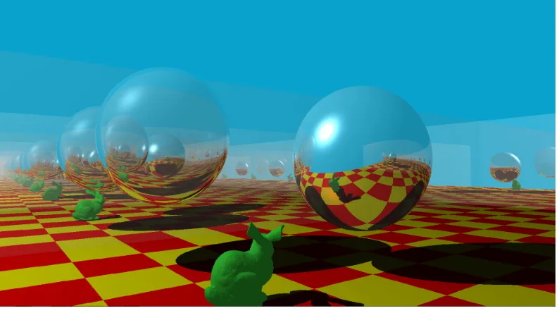
[image:13.612.113.510.257.479.2]Introduction
Figure 1.1: 1080p resolution ray-traced image generated using this framework.
Recent advances in consumer level parallel processing hardware have led to the feasibility of generating realistic computer graphics images at inter-active rates. However, even with high-end hardware, computationally de-manding rendering solutions such as ray-tracing must be heavily optimized to run in real-time.
region. These resources are wasted as the presence of such details does not impact the perceived quality of the scene due to reduced acuity in the peripheral region of the field of view. Raj et al. [22] noted however, that peripheral vision is not simply a blurred version of foveal vision; hence the traditional perceptual optimization approach of reducing spatial detail in the periphery still results in a noticeable reduction in image quality.
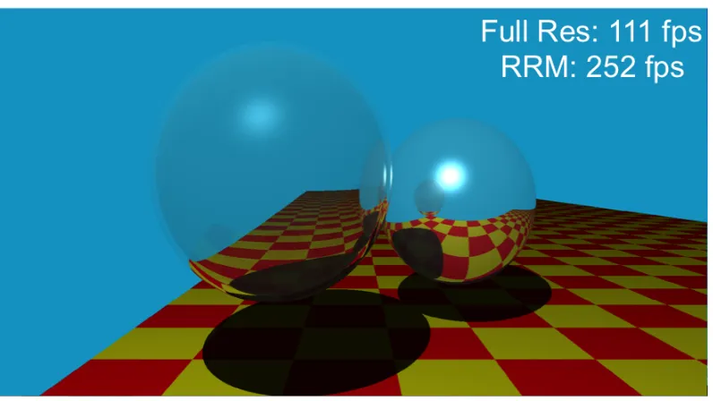
Figure 1.2: This framework renders the classic Whitted scene in 1080p at 111 fps in full resolution and 252 fps when RRM is enabled.
This thesis introduces refresh rate modulation (RRM), a novel perceptual optimization technique that produces better performance enhancement than spatial degradation techniques while more effectively preserving perceived image quality (Figure 1.2). Similar to variable resolution approaches, RRM partitions the display area into two subregions that correspond to the foveal and peripheral portions of the user’s field of view. However, instead of vary-ing samplvary-ing frequency, RRM adjusts the rate at which pixels are updated by the ray-tracer. The foveal region is updated once per frame, and therefore shows the scene in full detail at all times. Pixels in the peripheral region are refreshed once every N frames, where N can be adjusted to strike a balance between performance and perceived output quality.
that does not decrease the perceived quality of the overall image, but sig-nificantly increases performance. If the scene remains still for N or more frames, all peripheral pixels are refreshed and a full-detail image of the en-tire viewing area is rendered (the result of this behavior is shown in Fig-ure 1.1).
Within the framework, physics calculations may also be optimized through the use of real-time perceptual data. While the center of the field of view is able to detect errors in physical phenomena with high accuracy, the pe-riphery is less well-equipped to do so [20]. This means that collision er-ror tolerances can be significantly increased in regions outside of the fovea without reducing the perceived quality of motion (so long as penetrative er-rors are avoided). Many physics engines utilize acceleration structures for polygonal meshes that result in a series of successive calculations for colli-sion detection between two objects. If the collicolli-sion algorithm is modified to return a collision several layers earlier, computation for collisions with the mesh terminate early, and a computational speedup occurs.
Chapter 2
Background and Related Work
2.1
Human Visual Perception
The human visual system is made up of a complex set of sensory and pro-cessing organs that interact to produce sight. The visual process begins when light enters the eye through the pupil after bouncing off various sur-faces in the environment. The lens focuses light and directs it toward the back of the eye. A muscle surrounding the lens expands and contracts, changing the shape of the lens to match environmental conditions and en-abling variable focus. Light then travels through the vitreous humor, a trans-parent gel that fills the eye, to the retina on the rear wall.
The human retina contains a large number of interconnected receptor cells that intercept incoming photons and output electrical signals to the visual cortex. Cone cells provide color vision at high illumination levels, and are responsible for detail-oriented visual tasks. The distribution of cone cells across the retina is nonuniform (see Figure 2.1). Millions of these cells are packed into the macula, a small region at the center of the retina. The highest concentration of cone cells is in the center of the macula, the fovea centralis. While the fovea centralis accounts for less than one percent of total retinal area, approximately 50% of the information transmitted to the brain is generated by this region [24].
Figure 2.1: Distribution of cones in the retina. Adapted from [14]. Cones are densely packed in the center of gaze (fovea) and the density of cones falls off rapidly as angle from the center of gaze increases. The distribution of cones directly affects visual acuity. Visual acuity is highest in the center of gaze and falls off rapidly as angle from the center of gaze increases.
at any given time. For reference, the average person’s thumbnail is equiv-alent to a visual angle of 1.5◦–2◦ when held at arm’s length. In computer graphics terms, only three percent of a 21-inch computer monitor viewed at 60 centimeters lies within this region [5]. The visual system reorients the eye an average of three times per second via saccadic movement, and inte-grates the information gathered at each fixation point to create a composite perceived image that seems to be in full detail. Signals produced by the retina are transmitted via the optic nerve to the visual cortex, the region of the brain responsible for image processing [17].
[image:17.612.132.487.563.633.2]2.2
Eye Tracking
[image:18.612.139.487.245.378.2]The method most commonly used by current eye-tracking hardware is video-based infrared oculography. A light source emits infrared light toward the subject, which creates a series of four reflections on the eye, one each from the front and back of the cornea and lens. While all four reflections can be used to generate extremely precise fixation data, typically only the reflection from the front of the cornea is measured [5].
Figure 2.3: Monitoring distance between pupil center and corneal reflection yields viable fixation data [12].
2.3
Ray Tracing Algorithm
2.3.1 Overview
[image:19.612.126.497.366.650.2]Ray tracing is a physically based computer graphics technique that gener-ates images by shooting rays that begin at the eye point and travel through a viewing plane and into the scene (Figure 2.4). The basic algorithm creates one ray for each onscreen pixel. If a ray intersects an object in the scene, the associated pixel takes on the color of the object at the point of intersec-tion. Object color is determined using an illumination model that simulates diffuse and specular reflections. Shadows are handled by spawning an addi-tional ray towards each light source in the scene from an intersection point. If any object is between the light source and the point of intersection, that point is in shadow. If the object is reflective or transmissive, secondary rays are spawned recursively and contribute to the final color of the pixel.
2.3.2 Ray Definition
A ray is an infinite straight line that is defined by an origin point P0 and a unit vector direction D. For a viewing model with no antialiasing, one ray is spawned for every onscreen pixel, where the screen is represented by the view plane (Figure 2.5). The origin for all primary rays is the eye point, and the direction is calculated by drawing a line from the eye point to the center of the associated pixel and normalizing the resultant vector. For each frame, every ray must be tested for intersection with all scene objects to determine which color should be assigned to each onscreen pixel.
eye point
eye point
view
view
direction
direction
view plane
view plane
yw
[image:20.612.113.497.272.458.2]zw xw
Figure 2.5: One ray is generated for each onscreen pixel [29].
2.3.3 Ray-Object Intersection
Introduction
Ray-object intersection calculations are performed using formulas that are derived by substituting the parametric representation of a ray into geometric object equations. The parametric form of a ray is shown in (2.3). The quantity t represents the distance of an intersection from the origin of the ray at point P0 (2.1) in the normalized direction vectorD (2.2).
D = (dx, dy, dz) (2.2)
R = P0 +tD (2.3)
Splitting (2.3) intox, y, andz components yields the expressions shown in (2.4) through (2.6). This form is used to derive intersection formulas.
x = x0 +tdx (2.4)
y = y0 + tdy (2.5)
z = z0 +tdz (2.6)
Ray-Sphere Intersection
The simplest geometric object to intersect with a ray is the sphere. Sphere objects are used to encapsulate other objects for some acceleration tech-niques, as well as to render perfectly smooth parametric spheres that are not composed of polygons. (2.7) shows the basic equation for a point(xs, ys, zs)
on a sphere with center(xc, yc, zc) and radiusr.
(xs −xc)2 + (ys−yc)2 + (zs −zc)2 = r2 (2.7)
Substituting the parametric expressions from (2.4) through (2.6) for xs,
ys andzs in this equation yields (2.8) (whereA,B, andC are given in (2.9)
through (2.11).
At2 +Bt+ c = 0 (2.8)
A = dx2 +dy2 +dz2 (2.9)
B = 2(dx(x0 −xc) +dy(y0 −yc) +dz(z0 −zc))) (2.10)
C = (x0 −xc)2 + (y0 −yc)2 + (z0 −zc)2 −r2 (2.11)
Solving (2.8) fortproduces (2.12), the discriminant of which can be used to classify the intersection between the ray and sphere.
t = −B ± √
B2 −4C
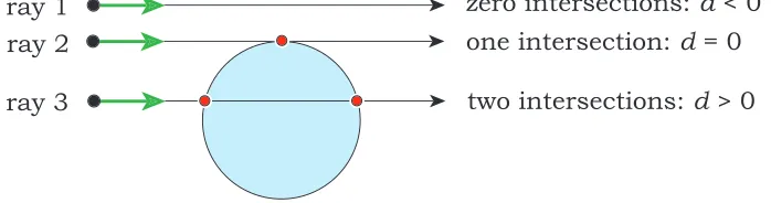
Figure 2.6 illustrates this classification process, which avoids an imagi-nary result for tand bypasses several floating point calculations in the case of no intersection. If d = B2 −4C is negative, there are no intersections and intersection computation can move on to the next object. If d is equal to 0, there is guaranteed to be only a single intersection. If dis greater than
0, two intersections exist, the closer of which should be used as it obscures
the farther intersection. Substituting the solution for tfrom (2.12) into (2.3) yields the point of intersection R = (xi, yi, zi).
ray 1 ray 2
ray 3
zero intersections: dd < 0
one intersection: dd = 0
two intersections:dd > 0
Figure 2.6: Ray-sphere intersection is characterized by the discriminant of (2.12) [29].
Ray-Triangle Intersection
Scene objects that are not parametrically defined are made up of groups of adjoining triangles. The ray-triangle intersection test begins by determining whether the ray passes through the plane defined by the triangle. (2.13) is used to find the distance from the ray origin to the point of intersection, where n is a vector normal to the triangle and p1 is a triangle vertex. If n ·D equals 0, the ray is parallel to the plane and there is no intersection.
If t is negative, the intersection occurs behind the eye point and is ignored (Figure 2.7). Otherwise, there is a valid intersection.
t= −(n·P0 −n·p1)
n·D (2.13)
Figure 2.7: Ray-triangle intersection begins by intersecting the plane in which the triangle lies. Adapted from [29].
sum is 360◦, the point is inside the triangle and the ray intersection is valid.
Otherwise, there is no intersection. Quadrilateral polygons are processed in a similar manner, with the fourth vertex added to the final angle calculation.
2.3.4 Illumination and Shading Models
Object color is determined using a combination of illumination and shading models. An illumination model describes the reflective characteristics of a surface, and impacts how light in the scene will interact with it. Illumination models serve as an approximation to the Bidirectional Reflectance Distribu-tion FuncDistribu-tion (BRDF, (2.14)), which relates reflected radiance (light emitted from a surface) in one directionω0 to irradiance (light incident on a surface) centered in another directionωi. Figure 2.8 illustrates the geometry involved
in the BRDF.
BRDF = fr(φi, θi, φr, θr) (2.14)
θi
n
surface
dω
reflected direction incoming
direction
i o
θo
φo φi
Figure 2.8: The BRDF relates reflected radiance to irradiance [29].
The diffuse component represents light that is scattered equally in all direc-tions from the point of contact. The specular component represents light that is perfectly reflected from the object to the viewer, and adds specular highlights. Figure 2.9 illustrates the effect of each of the three components on the final image.
Figure 2.9: Phong shading adds ambient, diffuse and specular light components to produce a realistic result [36]. (a) Ambient. (b) Diffuse. (c) Specular. (d) Combined.
The shading model uses the information generated by the illumination model to determine object color at each point. (2.15) shows the Phong shading formula, which uses the vectors shown in Figure 2.10 along with parameters for ambient (ka), diffuse, (kd) and specular (ks) response. Light
source (Li) and object colors (La) are also incorporated.
L(V) = kaLa+kdΣiLi(li ·n) + ksΣiLi(ri ·w0)ke (2.15)
θi θi
α l
n
r
o
Figure 2.10: Phong shading requires unit vectors for light source (l), surface normal (n), reflection (r) and viewing direction (w0) [29].
third terms in the Phong equation include a summation to account for multi-ple light sources with different positions and colors. The light source vector l and the reflection vector r will be different for each light source, while the viewing direction vector w0 and the normal vector nremain unchanged through the summation.
Shadows are produced by removing the diffuse and specular color com-ponents for points that are blocked from all light sources. After a valid intersection point is detected via the ray-object intersection tests, a shadow-ray is spawned towards each light source, and the shadow-ray-object intersections are repeated. If any object intersection that has a positive tvalue and is also not beyond the light source is found, the point is shadowed from that light source. Figure 2.11 illustrates shadow-ray generation.
2.3.5 Reflection and Transmission
For surfaces that are reflective or transmissive, additional color data must be added at the point of intersection to produce a realistic result. As shown in (2.16), these color data come in the form of reflection and transmission terms that are added to the result from the local illumination model. Objects have associated constants of reflection (kr) and transmission (kt) to indicate
shadow rays
a b
primary rays
Figure 2.11: Regions of shadow are found by spawning a shadow-ray toward each light source in the scene. If the ray intersects any object, the point is in shadow [29].
I = Ilocal +krIref lected +ktItransmitted (2.16)
A reflection ray is spawned when a ray intersects an object withkr > 0
(Figure 2.12). The direction of the reflected ray r is given by (2.17), with the origin at the point of intersection p. r0 is a unit vector indicating the direction from the viewing point to p.
θr θr r 0 r p n θr θr p n o r i= φo
φi=φo± !
[image:26.612.212.410.95.215.2](a) (b)
Figure 2.12: Reflected rayris spawned when rayr0intersects pointpon a surface that has a non-zero constant of reflection and surface normaln[29].
r = r0 −2( r0 ·n
||n2||)n (2.17)
limited to prevent performance issues for scenes with many reflective sur-faces, as only the first few reflections for a given surface have a perceptible impact on the image.
r 0 r 1 r 2 r 3 p'' p''' p' p
Figure 2.13: If a reflection ray intersects an object that is also reflective, another reflection ray is spawned at the point of intersection [29].
A transmission ray is spawned when a primary or secondary ray inter-sects a transparent object. Figure 2.14 illustrates the geometry of ray trans-mission. Snell’s Law is used to derive (2.18), which gives the direction of transmission ray t(transmission rays also begin at the point of intersection p). nit = nnoutin is the ratio of indices of refraction of the outer and inner media
[29]. Commonly depicted transmissive materials include glass (kt = 0.95)
and air (kt = 1.0).
t = nitw0 + (nit(−w0 ·n)− q
1 + (n2it((−w0 ·n)2 −1)))n (2.18)
2.3.6 Ray Tracing vs. Rasterization
The ray tracing algorithm is not widely used in real-time applications due to the large computational overhead that it incurs. However, since it models the physical behavior of light, it is able to handle a number of common but com-plex rendering situations in a simple and intuitive way. In most cases, it pro-duces better visual results than traditional rasterization while more closely approximating the actual behavior of real-world phenomena [29].
n
r
t i
θ θi
t
θ
o
φ
plane of incidence boundary
p
t
φ =φo± ! out
η
in
η
o
Figure 2.14: Transmission raytis spawned when rayw0intersects pointpon a surface that has a non-zero constant of transmission [29].
weak. Since the algorithm is not physically-based, environment maps must be used to approximate true reflection. While maps can be applied to curved objects, the map itself must be derived from a flat projection of the scene. One popular technique, cube projection, uses six virtual cameras to build projections for the walls, floor and ceiling of the cube (Figure 2.15). En-vironment mapping produces visually acceptable results, but it is strictly inferior to ray-traced reflection [2].
Transparency is another area in which ray tracing excels and rasteriza-tion falls short. Blending must be used to mimic true transparency for ras-terization. To achieve this, an opacity value is assigned to fragments as the associated polygons are rendered into the frame buffer. As shown in Figure 2.16, pixel color is calculated by adding together overlapping trans-parent objects, taking into account the opacity of each fragment and their arrangement. Creating realistic refraction effects is not possible with this technique.
Figure 2.15: Cube mapping. Adapted from [35]. (a) Sample scene with desired cube map center marked with a black dot. (b) Cube mapping as seen from viewpoint. (c) Cube map superimposed on original scene.
Figure 2.16: Blending. An opacity value is assigned to each polygon, and overlapping fragments are added together [2].
2.4
Ray-Tracing Acceleration Structures
During the development and implementation of the ray tracing algorithm, Whitted noted that approximately 75% of rendering time for simple scenes was allocated to ray-object intersections [31]. This percentage grows larger for more complex scenes, where the number of intersections per ray in-creases. Several techniques reduce the average number of intersection cal-culations per ray by organizing scene objects in such a way that each in-tersection test removes many objects from consideration. Such techniques include the bounding volume hierarchy, the uniform grid, the binary space partitioning tree and the k-d tree. Each technique exhibits different strengths and is best-suited to unique scene conditions and system design considera-tions.
2.4.1 Bounding Volume Hierarchy
In order to decrease the number of intersection calculations associated with each ray, the objects in the scene can be placed in simple bounding vol-umes. These volumes tend to have faster intersection algorithms, (e.g. a cube bounding volume for polygonal objects, Figure 2.17), and can contain multiple objects.
Figure 2.17: Objects surrounded by rectangular bounding volumes [10].
possibly intersect child volumes if it does not intersect the larger parent. At each level, up to half of the remaining nodes are eliminated from con-sideration. Using a bounding volume hierarchy can produce very good re-sults, with a best case performance ofO(log n)intersection calculations per
ray [10].
Figure 2.18: Bounding volume hierarchy [10].
For static scenes, performance of the construction algorithm is not ex-tremely important, as the hierarchy can be precomputed and then loaded at runtime. However, achieving a tree with near-optimal traversal efficiency is vital and can easily cause a 50x improvement in traversal performance over a suboptimal tree [31].
Hierarchy construction algorithms generally iterate over all objects in the scene and evaluate the traversal cost of placing the current object in a small set of available locations in the tree. The least costly location is selected, and the algorithm moves to the next object with the updated tree (Figure 2.19).
at each level. The tree is scored based on average traversal cost and stored in a buffer or written to disk. Another random tree is built and compared to the previous tree - if its score is higher, it replaces the current best tree. This process is repeated until either a traversal-cost tolerance is reached, or a set number of iterations has occurred. It can result in a close to optimal tree in much less time than brute force algorithms [31].
When designing a high-performance ray tracer, multiple acceleration techniques must be put in place. Doing so creates interconnected require-ments that affect the implementation of all techniques. The most impor-tant consideration is the ability to be easily represented to and computed by a GPU that operates under the current stream processor paradigm. The languages used to work with current GPUs generally conform to the C99 standard, which means that object oriented techniques are not available. In addition, recursive functions are not allowed. This means that the quality of an acceleration technique must take into consideration the unconventional issues that porting to a stream processor introduces.
Figure 2.19: Bounding volume hierarchy with escape indices [31].
algorithm, and in turn results in a very simple traversal algorithm for the GPU kernel.
Figure 2.20: Bounding volume hierarchy encoding data structure [31].
2.4.2 Uniform Grid
The uniform grid method splits the populated region of the scene into a regular three-dimensional grid with an arbitrary cell size. Cell size signif-icantly affects performance, and should be chosen based on the scale and distribution of the objects in the scene. A preprocessing algorithm assigns all objects to grid cells based on scene position [26].
When rendering takes place, the cells of the grid are traversed in order of their intersection with the current ray. The objects located within the first cell are checked for intersection with the ray. If an intersection is found, the remaining objects in the cell are tested and the algorithm returns that closest object in that cell. If an intersection is not found, the next cell is checked. This process continues until either a valid intersection is found or all populated cells have been depleted (Figure 2.21).
Figure 2.21: Ray-object intersection is guided by a regular three-dimensional grid. Each cell that the ray passes through is checked in order for intersecting objects. Traversal ends when a valid intersection is found.
2.4.3 Binary Space Partitioning Tree
The binary space-partitioning tree method involves recursively splitting the scene into two regions with an arbitrary plane. The goal of the splitting step is to create two equal groups of objects on either side of the plane. Once the two groups are created, a plane is calculated to split each into two new groups, with a subset of the objects located in each group. This process is repeated either until each group has a sufficiently small number of objects and is considered a leaf node, or until there is no plane that will cleanly split any of the current groups [6].
Figure 2.22 shows the binary space partitioning tree construction pro-cess. Group A, which contains all the polygons within the scene, is divided into groups B and C with an optimal splitting plane that results in the most even grouping possible. Group B is then recursively divided into groups E and D, and then group D is divided into groups G and F. At the end of this example, groups G and F are leaf nodes and contain two and three polygons, respectively. Groups E and C remain unfinished.
Figure 2.22: Binary space partitioning tree construction illustrated [34].
is also reduced, since the number of possible planes is greatly reduced due to the on-axis splitting plane restriction [6]. Enforcing this condition trans-forms the general binary space-partitioning tree into a special case called the k-d tree.
K-d Tree
Figure 2.23: The k-d tree is a special case of the binary space partitioning tree in which splitting planes must be on-axis [6].
also a major consideration. All splitting planes are perpendicular to one an-other, which decreases the computational intensity of ray-plane intersection tests [6].
For computation on a GPU device, the data structures for the BSP tree and k-d tree techniques can both be slightly modified to fit the GPU model used with the bounding volume hierarchy acceleration technique. Since re-cursion is not available on the GPU, traversal order must be encoded in a vector that is passed as an argument to the GPU. The splitting planes would make up the nodes shown in Figure 2.19 instead of bounding vol-umes. However, since there tend to be more splitting planes associated with a scene than bounding volumes, more storage space is required to articulate tree composition to the GPU. Performance suffers as a result [31].
2.5
OpenCL
2.5.1 Overview
In recent years, a computing trend has emerged that represents a shift from traditional serial processors towards parallel processors. This movement is driven by the capabilities and limits of the modern semiconductor manu-facturing process. While power consumption and heat generation issues re-strict traditional processor speed increases, parallel processors can achieve continued performance gains with reasonable power requirements and heat output (Figure 2.24). However, this paradigm shift introduces another is-sue; in order to take advantage of the additional computing power offered by parallel processors, programs must be written differently. Writing paral-lel, highly scalable code, which has been historically difficult for a number of reasons, is now absolutely required for high-performance applications.
Figure 2.24: GPU performance has rapidly outpaced CPU performance in recent years [19].
flavor of general-purpose processor that is less flexible than the CPU, but contains many more cores per die. Different manufacturers of parallel CPU and GPU architectures do not all subscribe to the same design philosophies, which has lead to an array of incompatible tools and programming mod-els that are required to program each architecture. This in turn leads to a substantial development cost increase for cross-platform projects. Several competing solutions exist to address this set of problems and streamline development for high-performance parallel architectures. These solutions include OpenCL and CUDA; OpenCL has been used for this thesis.
high-profile companies such as AMD, Apple, Intel and NVIDIA, among others. This wide support base ensures that the project remains current with respect to evolving parallel architectures. As with OpenGL, OpenCL pro-vides an API and a runtime system [28].
2.5.2 Platform Model
A hierarchical platform model is used to interface with heterogeneous hard-ware. As shown in Figure 2.25, the host device coordinates execution by transferring data to and from a set of compute devices (GPU, DSP, or mul-ticore CPU). Compute devices are each composed of an array of compute units, or cores, which are in turn made up of a number of processing ele-ments. Processing elements generally execute instructions as single instruc-tion, multiple data (SIMD) on CPUs and as single program, multiple data (SPMD) on GPUs. The model does not specify what hardware constitutes a compute device, so it is compatible with a variety of diverse hardware types including GPUs, multicore CPUs, and niche processors such as the Cell Broadband Engine [28].
2.5.3 Execution Model
The OpenCL execution model incorporates both task and data parallelism. Command queues facilitate the movement of data between the host and compute devices, and provide a means to specify dependencies between tasks to ensure that they are executed in the correct order. The OpenCL runtime executes tasks in parallel if all dependencies are satisfied. Tasks are comprised of kernels that apply a single function to a set of data elements in parallel. Synchronization and communication within a kernel are very restricted [28].
The kernel function is applied to a set of independent elements called work items. Work items acquire input data from the host according to an index assigned at queue-time, and each work item executes the same ker-nel function on its own data. Work items can be grouped together into work groups for local memory sharing and synchronization purposes (Fig-ure 2.26).
2.5.4 Memory Model
[image:40.612.169.451.328.617.2]The OpenCL memory model defines four regions of device memory ac-cessible to work-items during kernel execution. Figure 2.27 shows these regions, which include global, constant, local, and private memory. Global memory is accessible to all work items and work groups for both read and write. It is allocated by the host at runtime, and has a large capacity but rela-tively high memory latency. Constant memory is a subset of global memory that is still accessible to all work items, but only for read operations. Local memory is used for data sharing by work items in a work group, and allows read/write access for all items in the group. Private memory is accessible to only one work-item. Both local and private memory are allocated during kernel execution [27].
Host memory and compute device memory are independent of one an-other, which means that data must be explicitly moved from host memory to global memory to local memory and back. The host controls data move-ment by enqueuing read and write commands in the command queue [27]. Since memory operations between the host and the compute device are quite expensive, memory management commands should be kept to a minimum for optimum performance.
2.5.5 Executing an OpenCL Program
Figure 2.28 illustrates the process required to execute an OpenCL program. Several OpenCL devices can be leveraged simultaneously through the use of an OpenCL context, which also manages various OpenCL objects including command queues, memory constructs, program objects and kernel objects. In addition, the context is responsible for overseeing kernel execution.
The OpenCL runtime provides a compiler that is used to produce a pro-gram executable from OpenCL source code. Each OpenCL propro-gram must feature at least one kernel function, which is executed on many independent data members in parallel by the work units within the kernel. Utility func-tions may also be included and referenced in the kernel function. OpenCL programs are written in a modified version of the C99 standards, which includes several restrictions on recursive functions and function pointers. When moving from a traditional serial implementation to a parallelized OpenCL version, these restrictions can necessitate algorithm modifications to avoid illegal operations.
Figure 2.28: OpenCL programs are executed by the host through a series of steps that include compilation, data and argument creation, and transfer to the command queue [27].
The following procedure is used to initialize and execute a standard OpenCL program:
1. Query the host system for OpenCL devices 2. Create a context to associate OpenCL devices 3. Compile programs to run on OpenCL devices 4. Select program kernels to execute
5. Create memory objects in device memory 6. Copy input data to device memory
7. Provide arguments for each kernel
For programs that require multiple iterations of the same kernel, not all of these commands need to be issued for each execution. For instance, the OpenCL context object and program executable can remain active for the duration of program operation. Memory objects and kernel arguments are persistent, so constant inputs and arguments can be set once at program startup and left as-is for all kernel executions. For graphics programs, even output memory can be allocated once at startup and never be actively read back to the host. This is made possible by the device memory management scheme employed when OpenCL-OpenGL context sharing is used.
2.5.6 OpenCL-OpenGL Interoperability
OpenCL provides several functions that facilitate context sharing, which is the use of OpenGL buffers, textures and render buffer objects as OpenCL memory objects [8]. Context sharing allows the addition of an OpenCL ker-nel anywhere in the graphics pipeline. Memory buffers can be shared be-tween OpenCL and OpenGL with no data copy operations, and only minor overhead is incurred through context switching. An OpenCL reference ob-ject is created for existing OpenGL obob-jects, and ownership is transferred be-tween APIs before use [11]. Only one API at a time is permitted read/write access to the shared memory object.
Figure 2.29: Pixel Buffer Object. (a) Memory operation without PBO. (b) Memory opera-tion with PBO [1].
2.6
Previous Work
Computer graphics models that take advantage of the nonuniform acuity of the human visual system for computational speedup or data compres-sion have been proposed and implemented with positive results. While all systems use the same basic perceptual principle for detail reduction, the means of acquiring fixation data and reducing detail vary widely. The most straightforward approach is to use eye-tracking hardware to reduce spatial pixel resolution in regions of low acuity. More subtle methods exist that use a priori knowledge of scene contents and/or user task to reduce resolution in areas on which the user is unlikely to fixate for any length of time. Others still have foregone resolution degradation completely in favor of simplifying polygon meshes outside of the high-acuity region.
2.6.1 Foveal Pyramid
Geisler and Perry’s foveal pyramid approach [7] partitions an existing image into distinct regions based on their distance from the current region of inter-est. The resolution in each of the regions is reduced with a series of low-pass filters, resulting in a multi-resolution image that has full detail in the region of interest and decreases in resolution moving away from this region. Un-like most other techniques, this approach allows for a variable number of resolution levels to account for image content and viewing conditions.
hardware was used in Geisler and Perry’s implementation, it could be incor-porated for more accurate region of interest data. This algorithm achieves a 3x reduction in the amount of data required to represent an image (Fig-ure 2.30).
Figure 2.30: Foveal pyramid image encoding [7]. Resolution in an existing image is spa-tially reduced according to a model of human visual acuity.
2.6.2 Spatially Adaptive Ray Tracing
Levoy and Whitaker [13] implemented a spatially adaptive ray-tracing sys-tem that incorporates real-time fixation data from an eye tracker to produce a multi-resolution rendered image. Their 3D mip-map based algorithm re-sults in a nonuniform sampling distribution across the image plane, with considerably higher ray density in the foveal region.
Figure 2.3: Variable resolution ray tracing [10]. Ray density is reduced for areas outside of the fovea. A blurring effect is applied to reduce visible pixilation.
While no eye tracking hardware was used for this model (fixation was bound to the center of the image), Reddy emphasizes the need for such technology to produce an accurate perceptually based system.
A more general-purpose method for adaptive subdivision was proposed and implemented by Murphy and Duchowski [16]. It converts a full-polygon mesh to a variable level of detail mesh through spatial degradation accord-ing to visual angle. An eye tracker is used to determine which portion of the mesh to render in full detail while the remainder is rendered using the degraded mesh. For a 268,686 polygon Igea mesh, applying this technique allowed for near-interactive frame rates (20 - 30 fps), while frame rate for the full resolution model was too low to measure.
While many perceptual optimization techniques have shown positive re-sults, existing methods are not well-suited for application in a subtle, per-ceptually optimized real-time computer graphics architecture. Multi-resolution display models tend to produce noticeable image degradation; according to Levoy and Whitaker [10], “users are generally aware of the variable-resolution structure of the image”. In addition, the nonuniform pixel dis-tribution produced by the multi-resolution approach tends to exhibit poor
Figure 2.31: Variable resolution ray tracing [13]. Ray density is reduced for areas outside of the fovea. A blurring effect is applied to reduce visible pixilation.
2.6.3 Task-Based Level of Detail Adjustment
Certain features of a scene, such as edges, abrupt changes in color, and sud-den movement tend to attract involuntary user attention. Low-level saliency models determine which regions of a scene exhibit these features, and can be used as an alternative to eye-tracking when locating regions of interest. Cater et al. applied a saliency model that includes knowledge of a viewer’s visual task in order to render a scene with high resolution in regions of in-terest and lower resolution elsewhere [4]. Their approach takes advantage of inattentional blindness in addition to nonuniform visual acuity. This phe-nomenon causes users to fail to notice reduction in image quality in regions not related to the current task, even if those areas fall within the outer re-gion of the fovea. Their approach led to a rendering time of 5.4 hours for the 3072x3072 multi-resolution scene shown in Figure 2.32, compared to a time of 8.6 hours for the same scene in full resolution.
2.6.4 Adaptive Subdivision
Figure 2.32: Selective rendering with a task-level saliency model [4]. Resolution is reduced outside of predefined regions of interest that are selected based on user task.
that renders terrain geometry in high detail at the fixation point and a simpli-fied mesh outside of the foveal region [23]. This is accomplished by recur-sively subdividing the mesh, with regions outside of the fovea terminating earlier than those within. For a terrain model with 1.1 million triangles, the perceptual optimization achieved a 2.7x improvement in rendering time (Figure 2.33). While no eye tracking hardware was used for this model (fix-ation was bound to the center of the image), Reddy emphasizes the need for such technology to produce an accurate perceptually based system.
Figure 2.33: Adaptively subdivided terrain [23]. A low-polygon mesh is recursively sub-divided to produce higher detail in the foveal region. Subdivision terminates early in the periphery.
frame rate for the full resolution model was ”too low to measure”.
Figure 2.34: Adaptively subdivided model [18]. The full-detail mesh is simplified accord-ing to visual angle to generate an alternate low-detail mesh. A combined model is produced on the fly, with the full-detail mesh in the foveal region and the low-detail mesh elsewhere.
2.6.5 Limitations
employed by modern GPUs. Considering the current trend toward mas-sively parallel computing architectures, this is a major drawback.
Adaptive subdivision comes with a similar drawback; transitioning be-tween the full-detail mesh and the spatially degraded mesh produces motion that is very perceptible to the user’s peripheral vision. Task-level saliency models offer excellent computational speedup and low noticeability. How-ever, they are not applicable to the general case, where the user task may be complex and regions of interest are not guaranteed to be consistent or easily identifiable. Furthermore, automatic prediction of attention regions has been shown to be unreliable [15].
Chapter 3
System Design
3.1
Overview
The Perceptually Optimized Real-Time Computer Graphics framework was developed to take advantage of the nonuniform acuity of the human visual system for computational speedup in different graphics applications. Over the course of development, the novel Refresh Rate Modulation technique emerged as an effective means of achieving real-time frame rates with Whit-ted’s classic ray-tracing algorithm, and it became the primary area of inter-est. The main focus of this thesis is therefore the implementation of a high-performance GPGPU ray tracing engine that incorporates the novel RRM technique as well as more traditional acceleration techniques. A secondary investigation is conducted regarding the performance benefits of adjusting physics engine error tolerance for collisions in the user’s periphery.
3.2
Ray-Tracing Engine
3.2.1 Overview
Ray-tracing is a well-established method for rendering three-dimensional scenes [33]. The algorithm models the approximate path of light in reverse, flowing from the camera to objects in the scene. When a light ray inter-sects an object, the associated pixel is filled with the color of the object at that point. For reflective and refractive objects, additional rays are spawned recursively at the point of intersection.
historically prevented it from being used for real-time applications. Ap-proximately 75% of the time required to render simple scenes is allocated to computing ray-object intersections, with this number increasing for scenes with a large number of objects. A performance speedup can be realized by reducing the number of intersection tests per ray or the overall number of rays computed. This system is built on a basic ray-tracing framework, and is designed to reduce the number of rays that need to be computed by taking advantage of the differences in visual acuity between the foveal and peripheral vision. It also includes a number of traditional optimizations that reduce the number of intersections per ray as well as the time required to compute each intersection.
3.2.2 Structural Acceleration
The bounding volume hierarchy (BVH) is one effective method of orga-nizing scene object data to reduce ray-object intersection calculations per ray. Each polygon in a mesh is encapsulated within a bounding volume; the framework uses a sphere, which has a relatively low intersection cost. This set of volumes is paired and encapsulated within larger volumes un-til only one volume remains. This volume now contains a hierarchy that represents all geometry in the mesh. Ray intersections on the entire mesh are performed using the hierarchy. If a ray intersects the top level bound-ing sphere, its children are recursively checked for intersection. The BVH scheme eliminates all but one sphere intersection test for the majority of rays that do not actually intersect the mesh. See Section 2.4.1 for more details.
flattened BVH and triangle data are written to a file and loaded directly on subsequent executions to accelerate program startup.
Traversal of the hierarchy begins by intersecting the current ray with the top level bounding volume. If an intersection occurs, the counter used to index into the BVH array is incremented, which moves to the next bounding volume in the traversal. If there is no intersection, the counter is set to the node’s escape index to skip its children and move to its nearest sibling node. Traversal terminates either when the triangle within a leaf node is intersected, or when the rightmost bounding volume at any level is found to have no intersection with the current ray.
3.2.3 GPU Acceleration
General purpose GPU acceleration has emerged as a compelling means of reducing intersection computation time for high performance ray-tracing systems. This framework places all ray-tracing logic, including ray gen-eration, intersection tests, illumination, texturing and shading, in a single OpenCL kernel for execution on the GPU. A read-only input array of work unit structures holds coordinate data that tells each OpenCL work item into which onscreen pixel to write its result. Perceptual optimization leads to two separate pixel groups, which prevents the 1:1 correspondence between work items and onscreen pixels that would normally allow natural OpenCL kernel indexing to handle coordinates. Pixel work units are allocated once at the begin of operation, and are arranged in horizontal 4×1 strips for increased
coherency. A writable OpenGL Pixel Buffer Object (PBO) is shared with the OpenCL kernel and stores pixel data from each frame for display on-screen. The PBO remains in device memory throughout program execution, which bypasses costly GPU-CPU communication.
with hardcoded Boolean values in the kernel. While this implementation does sacrifice flexibility, the compiler is able to remove unused branches before runtime for improved performance.
3.2.4 Secondary Rays
A secondary ray stack is used to avoid the recursive function calls featured in the classic serial ray tracing algorithm. Each OpenCL work item has access to a private stack for secondary ray processing, the size of which depends on how many reflection and transmission rays need to be processed. While a large stack can be used to ensure sufficient space for most scenes, stack size is easily adjustable and should be tailored to match the current scene for optimum performance.
Private read and write pointers are maintained within each work item. The work item enters the stack after primary and secondary ray calculations are complete if secondary rays were added to the stack and reflection is enabled. When a secondary ray is spawned, it is stored in the stack and the write pointer is incremented. Each ray in the stack is processed in order and, if the ray intersects a reflective and/or transmissive object, new secondary rays are added to the stack. This continues either until the read pointer is equal to the write pointer, or until the capacity of the stack is exhausted.
Figure 3.1: Multi-pass secondary ray processing. Instead of using recursion or a secondary ray stack, multiple passes are made with the same OpenCL kernel.
2.3 with the stack-based approach). As such, further investigation is war-ranted.
[image:54.612.167.457.368.514.2]3.3
Perceptual Optimization
Figure 3.2: Runtime data flow. The framework is composed of several subsystems that work in tandem to produce perceptually optimized computer graphics.
rendering process for the next frame. Eye tracking hardware provides real-time fixation data in the form of X and Y screen coordinates, which are passed from the host to the OpenGL kernel to update foveal position. If physics functionality is enabled, the Bullet Physics engine drives positional data for all scene objects.
The eye-tracker used in this project is a Mirametrix S1 eye-tracking de-vice operating at 60 Hz with gaze position accuracy of less than 1◦. While
the data it provides are reasonably accurate, like all eye-trackers it does ex-hibit some degree of noise. Using raw fixation data detracts from the user experience, because peripheral vision is extremely sensitive to motion [16]. To rectify this issue, an auxiliary smoothing filter has been placed between the eye tracker and the host.
The standalone smoothing filter was developed by Sean Xu as part of his Eye Tracking Framework thesis project. The eye-tracking hardware broad-casts fixation data on a TCP socket in real-time, which is received by the filter and incorporated into a running average that is rebroadcast on a dif-ferent TCP socket. A thread spawned by the host connects to this socket and listens for updated fixation values. At the beginning of each frame, the current fixation value is provided to the OpenCL kernel as an argument so the onscreen foveal position can be adjusted.
3.4
Refresh Rate Modulation
Work units in each region are arranged in groups of four consecutive pixels (pixel strips) to maximize SIMD coherency and improve performance.
Figure 3.3: Work group layout. The display area is segmented into a dense inner region (the fovea) and a sparse outer region (the periphery). White pixels represent work units computed during a single frame
Figure 3.4 illustrates the Refresh Rate Modulation technique. A single pixel strip is processed at each frame, while the rest of the pixel strips in the refresh group maintain data from previous frames. When the red marker is reached, a full cycle is complete, and rendering for the next frame begins again at the green marker. Pixel strips in the foveal region undergo a full cycle each frame, so they are updated in real-time. Units in the peripheral region undergo a full cycle only once every N frames.
Applying the Refresh Rate Modulation technique leads to an effect in which the portion of the display that is viewed by the fovea is rendered in crisp detail, while the rest of the display is subtly fragmented. This frag-mentation occurs only when the camera or scene elements are in motion; if scene movement ceases, the display naturally resolves a full-detail image after N frames with no additional handling or overhead. This results in a full-resolution rendering after less than half a second for applications with a real-time frame rate.
Figure 3.4: Refresh rate modulation. Pixels in the foveal region are updated every frame for real-time rendering, while those in the peripheral region are updated less often for computational speedup. Refresh groups are composed of N pixel strips, where a pixel strip is defined as four adjacent pixels. One pixel strip in each work group is refreshed per frame in the peripheral region, where the individual pixel strip to be updated cycles between the N strips in the work group (which is why it takes N frames to resolve a full-resolution image when there is no scene motion). In this image, pixels are surrounded by a gray box, while sets of four pixels are grouped into pixel strips with a black box. Pixel strips that hold data from previous frame are outlined with dotted lines, while the single pixel strip that is being updated in the current frame is outlined with solid lines. N=12 for the refresh group shown here.
traditional spatial degradation techniques to reduce visible pixilation, and thereby prevents a great deal of processing overhead. Refresh order within the refresh groups can be adjusted on the fly to adjust fragmentation style for scene contents and movement, (e.g. horizontal, serpentine, scattered), and work group size may be decreased in real-time to reduce fragmentation in high-motion scenes or increased to maximize performance. Movement of the foveal region is accomplished within the GPU kernel by simply adding the current fixation position to each work unit position. This allows the en-tire input work group GPU memory buffer to remain unchanged throughout execution, and avoids costly CPU to GPU memory operations. The periph-eral region is also shifted in the same manner each frame. A refresh cycle offset is added to the coordinates of all work units in the peripheral region to update the appropriate pixels within the refresh group.
on the GPU, and enable fast data transfer to and from the graphics card through direct memory access (DMA) without CPU involvement [1]. Since the buffer is not flashed at the beginning of each frame, peripheral data from previous frames can be leveraged to provide meaningful context for the real-time contents of the foveal region.
The OpenCL kernel takes advantage of the lack of data dependency be-tween pixels in the ray-tracing algorithm to perform calculations for all pixels in parallel. Various data are passed to the kernel from the host for use with the ray-tracing algorithm, including fixation and camera position, frame dimensions, benchmarking parameters, and scene geometry. OpenCL automatically determines local work group size and distributes the workload among kernel work groups. Each work item in the kernel undergoes the fol-lowing process each frame:
1. Retrieve X and Y pixel coordinates from input work unit array.
2. Shift coordinates by fixation position (foveal group) or refresh cycle offset (peripheral group).
3. Calculate ray originating at eye point and passing through shifted co-ordinates.
4. Intersect ray with all spheres, all planes, and subset of triangles using bounding volume hierarchy - if no intersections are found, proceed to Step 7. Secondary ray data at point of intersection is calculated here. 5. Spawn shadow ray to light source.
6. Use intersection point, surface parameters from Step 4 and shadow data from Step 5 as input to Phong shading model.
7. Fill pixel with object color from Step 6 or background color from Step 4.
8. Store secondary rays in stack.
Once all work items have finished computation, the OpenCL kernel exits and returns control to the host. The host passes ownership of the shared PBO from OpenCL to OpenGL, and instructs OpenGL to write the contents to screen.
3.5
Issues Associated with Spatial Degradation
A more conventional multi-resolution ray-tracing framework was developed near the beginning of this project, and motivated development of the RRM technique. Analyzing performance differences between execution on the CPU and GPU yielded valuable insight regarding GPU characteristics as well as bottlenecks in the algorithm itself. Figure 3.5 shows a sample image from this original framework with a grid feature enabled to highlight the various resolution levels.
While results for this implementation were quite promising on the CPU and on an older commodity GPU, performance was less than impressive on a newer high-performance GPU. There were two primary reasons for this: complex CPU-side work group management between frames, and irregular work groups that are not well-suited to SIMD. In addition, this technique leads to pixilation even when there is no movement in the scene, which in turn requires a post-processing blur effect to remove visible seams. While post-processing effects can be achieved easily with the OpenGL Shading Language (GLSL), frequent switching between OpenCL and GLSL con-texts on the GPU is very costly and results in a massive performance drop. Observing these characteristics led to a focus on minimizing work group management, simplifying the work group layout and achieving acceptable perceived image quality without post-processing.
3.6
Perceptually Optimized Collision Detection
Figure 3.5: Spatial degradation results in less optimal performance and requires a costly blurring effect that is still noticeable to peripheral vision. (a) Whitted scene with grid to reveal multi-resolution layout (b) Whitted scene with blur. Static scene is shown for both images.
O’Sullivan [20] showed that interruptible collision detection can signifi-cantly reduce the time required for physics calculations while maintaining plausible scene motion. The system takes advantage of the bounding vol-ume hierarchy based collision detection system that Bullet Physics provides for use with static polygonal meshes. A performance improvement is gained by using only the top level of the BVH for collisions, which is subtle enough to be imperceptible to the periphery.
The Bullet Physics Library (BPL) automatically handles collisions be-tween a variety of object types, including the triangle meshes, planes, and spheres used in this framework [25]. On program startup, all scene object types, sizes and locations are registered with the BPL. Parameters such as object weight and world gravity are also provided at this time. At the begin-ning of each frame, the host (Figure 3.2) instructs the BPL to move forward one step in time. After object movement and collisions are processed by the BPL, the host retrieves updated object locations and passes them to the OpenCL kernel via a buffer in device memory.
new bounding volume hierarchy data at each frame for a moving mesh, the BPL requires that BVH meshes remain static. All spheres are subject to BPL gravity. If no spheres collide with the mesh for several consecutive frames, a negligible speedup will be realized as only the top level of the bounding volume hierarchy is queried. To avoid this, invisible collision planes are placed around the mesh and spheres.
Chapter 4
Results
4.1
Overview
The quality of a perceptual optimization technique must be assessed from two perspectives: computational speedup, and perceptual subtlety. The RRM approach requires a specialized metric for computational performance, since the onscreen position of the dense foveal region can have a pronounced effect on frame rate for scenes with nonuniform complexity. To account for this, one frame is rendered for each possible foveal position, and the results are averaged to produce a representative overall frame rate.
A number of benchmarks have been conducted to measure the perfor-mance impact of different aspects of the perceptual framework. All tests were performed on a system with a 3.6 GHz Intel Core i7 processor and a Radeon HD 7970 GPU, except where noted otherwise.
The perceptual subtlety of RRM was measured with a small pilot study. Subjects used the framework in full resolution mode and with RRM enabled, and rated the noticeability of RRM on rendered image periphery. The study also examined the effect of refresh group size on noticeability.
4.2
Benchmarks
4.2.1 Refresh Rate Modulation
In order to assess the overall effectiveness of Refresh Rate Modulation, frame rate measurements were taken for four scenes with and without RRM, with all acceleration techniques enabled. A 1920×1080 frame size was
used, with a foveal radius of 270 pixels and 3×4 (or N=12) refresh groups.
[image:63.612.116.501.276.567.2]These settings displayed the greatest balance between performance and per-ceptibility in preliminary tests.
Figure 4.1: Performance results for selected scenes rendered at 1080p resolution. (a) Whit-ted scene without secondary rays. (b) WhitWhit-ted scene with secondary rays. (c) High polygon scene without secondary rays. (d) High polygon scene with secondary rays. (f) Perfor-mance results for each scene at full resolution and with RRM enabled. A 3×4 refresh
group is used for RRM.
classic Whitted scene as well as a high polygon scene that features a 5,000-polygon model of the Stanford Bunny, each with and without secondary ray effects. The high polygon scene without secondary rays offers the best speedup. The framework handles the high polygon scene very well with RRM enabled, achieving a frame rate that is considerably better than real-time both with and without secondary rays.
4.2.2 Refresh Group Size
[image:64.612.127.497.389.613.2]Both performance and perceptibility tests were conducted for a variable re-fresh group size, since this parameter has a less intuitive impact on notice-ability than other factors such as fovea size. Figure 4.2 shows the perfor-mance impact when N is increased from the default of 12 to a maximum of 132 for the high polygon scene without secondary rays (Figure 4.1c). Frame rate shows a general upward trend, with a maximum increase of 50 fps. See Section 4.3.2 for perceptibility results.
4.2.3 Frame Resolution
As with any graphics application, the resolution of the rendering window has a large effect on frame rate since it alters the amount of information that must be calculated for each frame. Several tests were performed with common resolutions to quantify the magnitude of this effect on the frame-work both with and without RRM enabled. Figure 4.3 illustrates the rela-tive size of each resolution. As shown by the results in Figure 4.4, RRM is more effective for larger resolutions, with a maximum speedup of 3.62 for 1024×768 pixels. Raw frame rate peaks at 244 fps for an 800×600 frame
with RRM enabled. RRM has essentially no effect for the 640×480 frame
[image:65.612.132.495.315.398.2]size. This is likely due to lack of saturation on the GPU.
Figure 4.3: Relative frame sizes for common resolutions. (a) 1920×1080. (b) 1024×768.
(c) 800×600. (d) 640×480.
[image:65.612.161.462.476.647.2]4.2.4 Foveal Radius
Changing the size of the fovea also alters the volume of information that must be computed for each frame. A number of different foveal radii have been tested to establish the associated performance trend (Figure 4.5). All other RRM benchmarks use a foveal radius equal to 1
[image:66.612.128.498.228.447.2]4 of the frame height, (e.g., 270 pixels for a 1080p frame).
Figure 4.5: Performance of RRM for different foveal radii.
4.2.5 Bounding Volume Hierarchy
The bounding volume hierarchy greatly reduces the average number of in-tersection calculations per ray. Figure 4.6 shows the time required to render a single frame of the full resolution high polygon scene with reflection and transmission, both with and without BVH enabled.
When the BVH is used, the scene is rendered in real-time. When it is not used, rendering time increases to 10 seconds per frame. This illustrates that traditional structural acceleration is vital to achieving real-time results, even for a high performance GPGPU ray-tracing engine.
Figure 4.6: Impact of BVH technique on single frame render time for full-resolution high polygon scene with secondary rays.
4.2.6 Polygon Count
Figure 4.7 shows the performance of the framework for several different versions of the Stanford Dragon, which range from 5,000 triangles to 50,000 triangles at 640×480 resolution. Each model is shown in Figure 4.8 with
and without reflection and transmission enabled (frame rates for each are labeled). Secondary ray effects are cut short for the 50,000 triangle model due to the relatively small buffer capacity of local memory on current GPUs. Maximum secondary ray stack size is reduced from 20 to 5 for the 50,000 triangle model to avoid this issue.
Figure 4.7: Performance for Stanford Dragon model with different polygon counts.
4.2.7 Object Size
The onscreen size of a polygonal mesh has a large impact on performance. A small onscreen size can result in excellent performance even for ex-tr
![Figure 2.2: Visual angle describes the size of objects in the viewing region [5].](https://thumb-us.123doks.com/thumbv2/123dok_us/48684.4449/17.612.127.490.90.272/figure-visual-angle-describes-size-objects-viewing-region.webp)
![Figure 2.3: Monitoring distance between pupil center and corneal reflection yields viablefixation data [12].](https://thumb-us.123doks.com/thumbv2/123dok_us/48684.4449/18.612.139.487.245.378/figure-monitoring-distance-center-corneal-reection-yields-viablexation.webp)
![Figure 2.4: Rays are generated at the eye point and traced through the viewing plane andinto the scene [9].](https://thumb-us.123doks.com/thumbv2/123dok_us/48684.4449/19.612.126.497.366.650/figure-rays-generated-point-traced-viewing-plane-andinto.webp)
![Figure 2.12: Reflected ray(a) (b) r is spawned when ray r0 intersects point p on a surface that hasa non-zero constant of reflection and surface normal n [29].](https://thumb-us.123doks.com/thumbv2/123dok_us/48684.4449/26.612.212.410.95.215/figure-reected-spawned-intersects-surface-constant-reection-surface.webp)
![Figure 2.15: Cube mapping. Adapted from [35]. (a) Sample scene with desired cube mapcenter marked with a black dot](https://thumb-us.123doks.com/thumbv2/123dok_us/48684.4449/29.612.148.473.89.456/figure-cube-mapping-adapted-sample-desired-mapcenter-marked.webp)
![Figure 2.16: Blending. An opacity value is assigned to each polygon, and overlappingfragments are added together [2].](https://thumb-us.123doks.com/thumbv2/123dok_us/48684.4449/30.612.218.401.90.199/figure-blending-opacity-value-assigned-polygon-overlappingfragments-added.webp)
