Scaling lightness perception and differences above and below diffuse white and modifying color spaces for high-dynamic-range scenes and images

Rochester Institute of Technology

RIT Scholar Works

Theses Thesis/Dissertation Collections

2011

Scaling lightness perception and differences above

and below diffuse white and modifying color

spaces for high-dynamic-range scenes and images

Follow this and additional works at:http://scholarworks.rit.edu/theses

This Thesis is brought to you for free and open access by the Thesis/Dissertation Collections at RIT Scholar Works. It has been accepted for inclusion in Theses by an authorized administrator of RIT Scholar Works. For more information, please [email protected].

Recommended Citation

Scaling Lightness Perception and Differences Above and Below Diffuse White and

Modifying Color Spaces for High-Dynamic-Range Scenes and Images

by

Ping-hsu Chen

B.S. Shih Hsin University, Taipei, Taiwan (2001)

M.S. Shih Hsin University, Taipei, Taiwan (2003)

A thesis submitted in partial fulfillment of the requirements for the degree of Master of Science

in Color Science in the Center for Imaging Science, Rochester Institute of Technology

Signature of the Author

Accepted By

CHESTER F. CARLSON CENTER FOR IMAGING SCIENCE

COLLEE OF SCIENCE

ROCHESTER INSTITUTE OF TECHNOLOGY

ROCHESTER, NY

CERTIFICATE OF APPROVAL

M.S. DEGREE THESIS

The M.S. Degree Thesis of Ping-hsu Chen

has been examined and approved by two members of the

Color Science faculty as satisfactory for the thesis

requirement for the Master of Science degree

Prof. Mark D. Fairchild, Thesis Advisor

Scaling Lightness Perception and Differences Above and Below Diffuse White and

Modifying Color Spaces for High-Dynamic-Range Scenes and Images

Ping-hsu Chen

A thesis submitted in partial fulfillment of the requirements for the degree of Master of Science

in Color Science in the Center for Imaging Science, Rochester Institute of Technology

Abstract:

The first purpose of this thesis was to design and complete psychophysical experiments for scaling

lightness and lightness differences for achromatic percepts above and below the lightness of diffuse

white (L*=100). Below diffuse white experiments were conducted under reference conditions

recommended by CIE for color difference research. Overall a range of CIELAB lightness values from 7

to 183 was investigated. Psychophysical techniques of partition scaling and constant stimuli were

applied for scaling lightness perception and differences, respectively. The results indicate that the

existing L* and CIEDE2000-weighting functions approximately predict the trends, but don’t well fit the

visual data. Hence, three optimized functions are proposed, including a lightness function, a

lightness-difference weighting function for the wide range, and a lightness-lightness-difference weighting function for the

range below diffuse white. The second purpose of this thesis was to modify the color spaces for

high-dynamic-range scenes and images. Traditional color spaces have been widely used in a variety of

applications including digital color imaging, color image quality, and color management. These spaces,

however, were designed for the domain of color stimuli typically encountered with reflecting objects and

image displays of such objects. This means the domain of stimuli with luminance levels from slightly

above zero to that of a perfect diffuse white (or display white point). This limits the applicability of such

at zero luminance/lightness and by their uncertain applicability for colors brighter than diffuse white.

To address HDR applications, two new color spaces were recently proposed by Fairchild and Wyble:

hdr-CIELAB and hdr-IPT. They are based on replacing the power-function nonlinearities in CIELAB

and IPT with more physiologically plausible hyperbolic functions optimized to most closely simulate the

original color spaces in the diffuse reflecting color domain. This thesis presents the formulation of the

new models, evaluations using Munsell data in comparison with CIELAB, IPT, and CIECAM02, two sets

of lightness-scaling data above diffuse white, and various possible formulations of hdr-CIELAB and

ACKNOWLEDGEMENTS

I would like to express my deepest gratitude to my advisor, Dr. Mark D. Fairchild, for his excellent

guidance and patience. I would never have been able to finish my thesis without his great help.

I would like to thank Dr. Roy S. Berns, who gave me the opportunity to study at the Munsell Color

Science Laboratory and financially supported my research.

I would also like to thank Dr. Jim Ferwerda, Dr. David R. Wyble, Mr. Jonathan Phillips, Mr. Lawrence

A. Taplin, and Mr. Max Derhak for guiding my research, and helping me develop my background in

color science. Special thanks goes to Val Hemink, who was the best lab mom in the world.

I would like to thank Rod Heckaman, Erin Fredericks, Ben Darling, Dan Zhang, Jun Jiang, Koichi

Takase, David Long, Marissa Haddock, Susan Farnand, Brian Gamm, and Hao Li, who were always

willing to help and offer their best suggestions. Many thanks to all my observers who kindly volunteered

their time.

I would also like to thank my parents, sisters, and brother. They were always extremely supportive and

encouraging.

TABLE OF CONTENTS

1. INTRODUCTION ...1

1.1 Overview of Wide Range Scaling Lightness Perception and Lightness Difference ...1

1.2 Overview of High-Dynamic-Range Color Space ...2

1.3 Purpose of this Thesis ...3

2. SCALING LIGHTNESS PERCEPTION ABOVE AND BELOW DIFFUSE WHITE ...4

2.1 Introduction...4

2.2 Effects on Lightness Perception...7

2.3 Method of Partition Scaling...9

2.3.1 Experimental uncertainty of method of partition scaling ... 9

2.4 Experimental Designs ...10

2.4.1 Experiments for 10-degree visual field...10

2.4.2 Experiments for 2-degree visual field ...15

2.5 Results and Discussion...21

2.6 Conclusions...30

3. SCALING LIGHTNESS DIFFERENCE ABOVE AND BELOW DIFFUSE WHITE ...31

3.1 Introduction...31

3.2 Method of Constant Stimuli ...31

3.3 Lightness Weighting Functions ...35

3.4 Experimental Designs ...36

3.4.1 New experiments for a range both above and below diffuse white, DE>100...36

3.4.2 Traditional experiment for a range below diffuse white, DE<100 ... 38

3.6 Conclusions...43

4. COLOR SPACES FOR HIGH-DYNAMIC-RANGE SCENES AND IMAGES...45

4.1 Introduction...45

4.2 Derivation and Formulation of hdr-CIELAB ...46

4.3 Derivation and Formulation of hdr-IPT ...51

4.4 Appearance Predictions of Munsell Colors...53

4.5 Wide-Range Lightness Predictions...60

4.6 Conclusions...64

5. CONCLUSIONS AND FUTURE RESEARCH...65

6. REFERENCES...66

LIST OF FIGURES

Figure 2.1: The typical response compression of lightness perception illustrated by the Munsell Value

scale, CIELAB L*, and a simple cube-root function. ...5

Figure 2.2: Lightness scales with the influence of crispening for backgrounds with different relative luminance levels according to Semmelroth’s equation...8

Figure 2.3: Configuration of SL1>100 and SL1<100 lightness scaling experiments...11

Figure 2.4: The setup of SL1>100 and SL1<100 lightness scaling experiments in a dark room...12

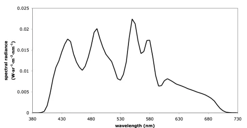
Figure 2.5: The spectral radiance of the projector for the SL1>100 and SL1<100 lightness scaling experiments...13

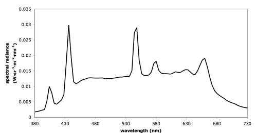
Figure 2.6: The spectral radiance of the light source of the experiments for 2-degree visual field...16

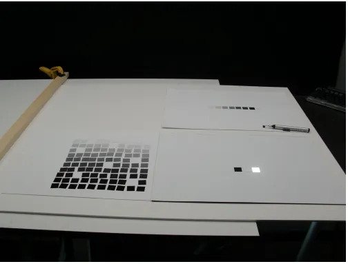
Figure 2.7: The experimental setup for SL2<100 ...17

Figure 2.8: The experimental setup for SL2>100. ...20

Figure 2.9: The visual data of all 50 observers for SL1 experiments...23

Figure 2.10: The visual data, optimized lightness scale, and CIELAB lightness function. ...24

Figure 2.11: The visual data of all 17 observers for SL2 experiments...28

Figure 2.12: The visual data, optimized lightness scales, and CIELAB lightness function...29

Figure 3.1: An example for applying the 3-by-1 low-pass filter algorithm to correct the non-monotonic responses...32

Figure 3.2: The configuration of lightness difference scaling experiment (DE>100). ...36

Figure 4.1: An HDR scene...46

Figure 4.2: SL2 visual data for finding the turning point from the linear range to the nonlinear decay in a log-log coordinate ...48

Figure 4.3: CIELAB L* and fitted Michaelis-Menten functions of relative luminance in the range from 0-4...50

Figure 4.4: IPT I and fitted Michaelis-Menten functions of relative luminance in the range from 0-4....52

Figure 4.5: Model lightness predictors as a function of Munsell Value...55

Figure 4.6: Model chroma predictors as a function of Munsell Chroma...56

Figure 4.7: Model chroma predictors as a function of Munsell Chroma...57

Figure 4.8: Visualization of PCA analysis on the dimensionality of constant hue lines...58

Figure 4.9: Results of t-tests on hue spacing...59

Figure 4.10: Prediction of lightness scaling data in a wide lightness range. Visual data are shown with their error bars for 95% confidence limit. ...61

Figure 4.11: Prediction of lightness scaling data in the range from L*=0 to L*=100...61

Figure 4.12: Prediction of lightness scaling data in a wide lightness range. ...63

Figure A.1: The probit fit of color centers for DE>100 experiment ...79

LIST OF TABLES

Table 2.1: Partial visual data of the Munsell 1933 lightness scaling experiments (10 x Values !L*)...10

Table 2.2: Visual data of the lightness scaling experiments, SL1>100 and SL1<100...21

Table 2.3: Mean visual data of the lightness scaling experiments, SL2>100 and SL2<100...26

Table 3.1: Summary of the tolerance analysis results of DE>100 and DE<100 experiments. It includes the color center position, unit color vector ("L*, "a*, "b*, first eigenvalue), method of tolerance determination (Probit or 3D Normit), tolerance (T50) with upper and lower fiducial limits (UFL, LFL), standard error for uncertainty, standard deviation (S), chi-square value ( ! "2), heterogeneity factor (h), t value, and ±T50s...40

Table 4.1: The R2 value of fitted linear line for visual data ranged from the darkest one to itself...47

Table 4.2: Two sets of mean experimental data on scaling lightness above diffuse white. ...60

Table A.1: Colorimetric values and visual responses for DE>100 experiment...75

Table A.2: Colorimetric values and visual responses for DE<100 experiment...77

Table A.3: Discrimination data for DE>100 experiment ...81

1. INTRODUCTION

1.1 Overview of Wide Range Scaling Lightness Perception and Lightness Difference

The CIELAB L* cube-root-based function, recommended by CIE in 1976, is commonly used to

compute correlates of the lightness perception [CIE Publ. 15.2, 1986]. However, it is possible to

compute lightness values greater than that of diffuse white (L*>100), such as when encountering

fluorescent materials or high-dynamic-range images. Specularities on glossy materials might also appear

lighter than diffuse white when viewing them with different viewing geometries. However, the CIELAB

equation has no established psychophysical meaning when L* values exceed 100. There are seldom

psychophysical experiments for scaling lightness perceptions exceeding diffuse white. As a result,

conditions such as measuring and viewing geometries of materials are carefully controlled to avoid

specular reflection in traditional colorimetric applications. There has been a growing interest, for both

material specification and HDR imaging, in how to calculate meaningful perceptual magnitudes for a

wider lightness range.

Lightness discrimination data for a wider range are also necessary, since most of the visual tolerance

data are derived from samples darker than diffuse white and the detailed relationship between lightness

discrimination and lightness level, as modeled in CIEDE2000, requires more data for verification.

This thesis presents six sets of scaling experiments. The first and second experiments are designed to

scale lightness perception for a range above and below diffuse white and are denoted by “SL1>100” and

“SL1<100”, respectively. The third and fourth experiments are also designed to scale lightness

perception, but with an experimental configuration to better control the adaptation point. They are

denoted by “SL2<100” and “SL2>100” for a range below and above diffuse white, respectively. The

fifth and sixth experiments are intended for scaling lightness differences for a range above and below

DE>100 experiments were conducted together under similar viewing environments. The DE<100

experiment was conducted under CIE reference viewing conditions.

1.2 Overview of High-Dynamic-Range Color Space

Traditional color spaces such as the CIE 1976 L*a*b* Color Space, CIELAB, and the IPT space

optimized for hue linearity have been widely and successfully used in a variety of applications including

digital color imaging, color image quality, and color management. These spaces, however, were

designed for the domain of color stimuli typically encountered with reflecting objects and image

displays of such objects. More specifically, this means stimuli with luminance levels from slightly above

zero to that of a perfect diffuse white (or display white point), or dynamic ranges of approximately

100:1. This limits the applicability of both of these spaces to color and image quality problems in HDR

imaging. This is caused by their hard intercepts at zero luminance/lightness that disregards the visual

noise and by their uncertain applicability for colors brighter than diffuse white. To address these HDR

questions, two newly formulated color spaces were recently proposed for further testing and refinement,

hdr-CIELAB and hdr-IPT [Fairchild, 2010]. They are based on replacing the power-function

nonlinearities in CIELAB and IPT with more physiologically plausible hyperbolic functions, based on

the Michaelis-Menten equation, optimized to most closely simulate the original color spaces in the

diffuse reflecting color domain.

In addition, experiments SL1>100 and SL1<100 have been completed to scale lightness and

lightness differences in the range well above the lightness of diffuse white. Overall a range of CIELAB

lightness values from 7 to 183 was investigated. The results indicated that the existing L* and

[Chen, 2010]. Those data were well predicted by the hdr-CIELAB and hdr-IPT models for the range of

lightness below diffuse white, but lightness was under predicted by the models above diffuse white.

New psychophysical experiments SL2>100 and SL2<100 have been completed to more carefully

study lightness perception in the CIELAB L* range from zero to 200, with smaller stimuli (about 2-deg.)

on a larger white background to better control the adaptation point. The new data also suggest that the

hdr-CIELAB and hdr-IPT models under predict lightness above that of diffuse white. The data also

show a clear crispening effect around the white-point lightness.

These results suggest that the formulation of the hdr- color spaces might require an adjustment for

the background lightness that moves the semi-saturation point up to the lightness of diffuse white rather

than fixing it at the lightness of middle gray as in the original formulation. This may result in color

spaces that are more effective for HDR applications, but more different from the original LDR color

spaces.

This thesis presents the formulation of the proposed models along with some evaluations using

Munsell data in comparison with CIELAB, IPT, and CIECAM02. It also describes both sets of

experimental data on scaling lightness above diffuse white and various formulations of hdr-CIELAB and

hdr-IPT to predict the results.

1.3 Purpose of this Thesis

The purpose of this research was to design and complete psychophysical experiments for scaling

lightness for a range both above and below the lightness of diffuse white, and to create CIELAB-like

color spaces that will be capable of describing the appearance of high-dynamic-range scenes and images

2. SCALING LIGHTNESS PERCEPTION ABOVE AND BELOW DIFFUSE WHITE

2.1 Introduction

Three terms from the International Lighting Vocabulary are used to scientifically define the lightness

and brightness [Fairchild, 1995a]. These are:

Luminance: A physical measure of the stimulus with unit of cd/m2.

Brightness: Attribute of a visual sensation according to which an area appears to emit more or

less light.

Lightness: The brightness of an area judged relative to the brightness of a similarly illuminated

area that appears white or highly transmitting.

The lightness scale can be approximately described by Stevens’ power-law [1961] to correlate the

perceptual magnitude and the stimulus that evokes it. Prior to Stevens, the power relationship was also

suggested by Godlove [1933] to describe one of the most well-known and utilized lightness scales, the

Munsell Value scale [Long, 2001]. Generally, the power relationship represents the common feature of

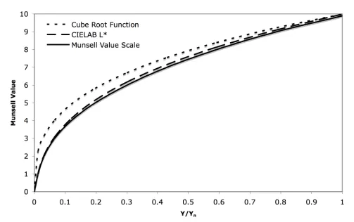
response compression in lightness scales. This is illustrated in Figure 2.1 with the example of the

Munsell Value scale, where the CIELAB lightness equation exhibits a good approximation. CIELAB L*

is scaled by a factor of 0.1 in the figure because Munsell Value is approximately 0.1L*. The CIELAB

lightness equation, shown in Equation (2.1), is a modification from the simple cube-root power function

to avoid infinite slope at zero luminance and improve fitting the Value scale. It is worth noting that a

simple cube-root power function does not well describe the Value scale.

!

L*

=116f(Y/Yn)"16 f(x)= x

1/ 3

x>0.008856 7.797x+16 /116 x#0.008856

$ % &

(2.1)

Figure 2.1: The typical response compression of lightness perception illustrated by the Munsell Value scale, CIELAB L*, and a simple cube-root function.

The Munsell Value scale was an early system to have both deliberate physical and perceptual

definitions; hence, several formulae have been derived to calculate the Munsell Value, V, from

luminance factor, Y/Yn. Priest [1920] applied a square root, shown in Equation (2.2), to fit the visual

observations with a white background.

!

V =10(Y/Y_n)1/ 2 (2.2)

Subsequently, in order to take into account induction effects caused by background lightness,

formulae were derived to fit the visual observations with a middle-gray background. One such

formulation, shown in Equation (2.3), was suggested by Munsell et al. [Godlove, 1933; Munsell, 1933].

Another formula, shown in Equation (2.4), was proposed by Hemmendinger [1980] and McLaren [1980]

look-up table or an analytic expression from McCamy[1992] is used for the inverse calculation of the

fifth-order polynomial.

!

V =(1.474(Y/Y_n)"0.00474(Y/Y_n)2₎1/ 2 _(2.3)

!

Y/Y_n =1.1913V "0.22532V2

+0.2351V3

"0.020483V4

+0.00081935V5 (2.4)

Since a formula based on the cube-root power function is easily invertible and fits the visual data

well, the CIE recommended the CIELAB lightness scale with a cube-root-based function as shown in

Equation (2.1). Two additional formulae for different background luminance levels were proposed by

Foss [1944] and Richter [1953; 1955]. Foss’s formula, Equation (2.5), was derived from the

observations on a gray background with a “sliding” luminance factor close to that of the lightness

difference pair. Richter’s formula, Equation (2.6), applied best for background luminance factors close

to 50% [Wyszecki, 2000a].

!

V =0.25+5log10(100Y/Yn) (2.5)

!

V =6.1723log10(40.7(Y/Yn)+1) (2.6)

The reason to have several lightness scale models is that lightness perception is highly dependent on

the luminance factor of the background, the level of illumination, stimuli configuration, sample size, and

many other factors. Each formula applies best for its corresponding viewing condition. The Munsell

Value scale is often cited as a perceptually uniform lightness scale for small patches on a medium-gray

background. Hence, it is important to note that the CIELAB lightness function, derived by fitting the

Munsell Value scale, is best applied for that viewing condition. Under different viewing conditions, a

color appearance model such as CIECAM02 with viewing condition parameters is required to predict

2.2 Effects on Lightness Perception

As the optimal power-function exponent would be altered for different observers, experimental

designs, and viewing condition [Fairchild, 1995a; Wyszecki, 2000b; Berns, 2000a], those effects

influencing lightness perception should be well understood and controlled when designing a lightness

scaling experiment and analyzing the data. Fairchild [2005] listed a series of color appearance

phenomena that influence lightness perception. Simultaneous contrast, also referred to as lightness

induction, is an effect that the perceived lightness of a stimulus changes with the relative luminance of

the background. For instance, a gray stimulus looks lighter when it is placed on a darker background,

and vice versa. Therefore, in order to control this effect, the backgrounds of stimuli are usually carefully

controlled in a set of experiments.

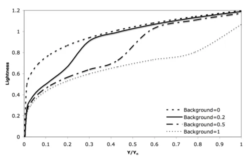
Crispening is an effect where the perceived lightness difference between two stimuli is greater when

viewed on a background with similar luminance. Takasaki [1966] and Semmelroth [1970] developed

equations to model the crispening effect for backgrounds with different luminance levels. According to

Semmelroth’s equations, lightness scales, illustrated in Figure 2.2, exhibit a sharp increase in the slope

of the curves due to crispening, and an overall shift of lightness magnitude due to simultaneous contrast.

Recalling that the Munsell Value scale is cited as a uniform scale for small patches on a medium-gray

background, however, it is clear that the CIELAB L* function doesn’t reveal the crispening effect by

comparing the curve of the Munsell Value scale in Figure 2.1 and the curve of background luminance

factor YB = 0.2 in Figure 2.2. Semmelroth [1971] demonstrated the nonuniformities of the Munsell

Value scale, regardless of whether the background is presented as a medium-gray or a sliding luminance

factor half way between two judged stimuli. This also implies nonuniformities of CIELAB lightness

Figure 2.2: Lightness scales with the influence of crispening for backgrounds with different relative luminance levels according to Semmelroth’s equation.

The overall luminance level and the surround-relative luminance significantly influence lightness

perception [Stevens, 1963; Bartleson, 1967] as described by the Stevens effect and the

Bartleson-Breneman equations, respectively. The perceived contrast, which correlates with the exponent of a

lightness power-function, altered luminance level and surround relative luminance. In addition, the

observers’ state of adaptation also affects lightness perception [Stevens, 1963]. Sixty seconds are the

suggested duration for observers to adapt to a viewing condition when luminance is not significantly

changed [Fairchild, 1995b]. Moreover, the influences of sample size and stimulus configuration should

be noted. Simultaneous contrast and crispening effects are more significant for smaller samples

viewing conditions with changes of background and surround luminance level and stimulus

configuration, thus requiring a more complex function to describe the visual results [Bartleson, 1967]. In

lightness scaling experiments, background has a very large influence on the results. It is necessary to

obtain the background information and the viewing condition details when interpreting lightness scales

and psychophysical results. It is desirable to choose data and scales obtained with similar viewing

conditions when implementing a comparison.

2.3 Method of Partition Scaling

Experiments scaling lightness perception are intended to derive a ratio scale to correlate perceptual

magnitudes of lightness attributes and physical measures of stimuli. The method of partition scaling,

also known as method of bisection, has been successfully used to develop lightness scales. With two

presented stimuli, A and B, the observer is asked to select a third stimulus, C, such that the lightness

difference between A and B is equal to the lightness difference between B and C, or the lightness of C is

half way between A and B. A uniform lightness scale is obtained by conducting the experiment

successively through the lightness range of interest.

2.3.1 Experimental uncertainty of method of partition scaling

Munsell et al. [Munsell, 1933] pointed out that it is difficult for observers to select the midpoint in

sensation between two stimuli that differ greatly. This difficulty can cause higher uncertainty for the

partition scaling experiment than the just-noticeable-difference (JND) experiment. However, Munsell et

al. lowered the uncertainty by the experimental design of subdividing the sensation interval into a

number of smaller intervals and presenting them together. This design allowed observers to compare

adjustment easier. They reported that the uncertainty was either similar to or better than that of the JND

method. One set of the visual data presented in their research is listed in the Table 2.1. Note these data

were used to validate the JND results, not to specify the Munsell value scale [Berns, 1985]. Data in

Table 2.1 were derived from the partition scaling experiment and included sufficient data (14 observers)

for calculating the meaningful value of the estimated standard error of mean with the Equation (2.7).

!

S_e= S

N (2.7)

where S is the sample standard deviation (

!

S= 1

N"1 (xi"x)

2

i=1 N

#

Basically, the uncertainty (standard error) increases as the lightness increases, and is between 0.8 and

1.3 for the range lighter than mid-grey.

Table 2.1: Partial visual data of the Munsell 1933 lightness scaling experiments (10 x Values ! L*)

2.4 Experimental Designs

2.4.1 Experiments for 10-degree visual field

Experiment 1: Scaling lightness perception for a range exceeding diffuse white, SL1>100

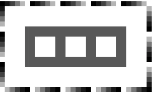
The method of partition scaling was used in the lightness scaling experiments. The stimulus

configuration of the experiment is shown in Figure 2.3. It was printed with Felix Schoeller glossy paper

with achromatic inks, and fastened to the wall in a darkened room. Outside the configuration, there was

Value #1 #2 #3 #4 #5 #6 #7 #8 #9 #10 #11 #12 #13 #14 Mean Se

9.63 88.3 88.3 88.3 88.3 88.3 88.3 88.3 88.3 88.3 88.3 88.3 88.3 88.3 88.3 88.3 0.0 8.68 61.6 65.5 61.6 65.5 70.0 64.6 64.6 70.0 64.6 74.2 74.4 74.2 74.2 74.4 68.5 1.3 7.73 46.3 50.8 46.3 48.3 53.6 48.3 50.4 50.4 48.3 56.0 52.7 50.8 58.5 52.4 50.9 0.9 6.77 34.1 35.6 32.3 34.1 35.6 35.0 35.6 34.1 34.1 43.5 35.4 35.0 43.7 38.7 36.2 0.9 5.82 25.3 27.3 22.3 25.3 22.3 25.3 26.4 25.3 25.3 32.2 25.3 26.4 31.8 26.9 26.2 0.8 4.86 18.5 16.6 14.6 13.2 14.6 18.5 17.4 18.5 17.4 22.3 17.9 17.4 22.3 17.9 17.7 0.7 3.91 13.0 9.7 9.7 8.8 8.8 11.7 10.7 10.7 11.7 13.2 13.0 10.7 15.6 10.2 11.3 0.5

2.95 6.4 6.2 6.4 5.1 4.8 6.2 6.2 6.4 5.6 6.2 6.7 6.2 7.8 5.0 6.1 0.2

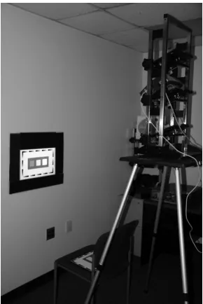
a frame of black foam-core board. The experimental setup is shown in Figure 2.4. A Planar PR5022

DLP projector, above the observer with a geometry of 45º/0º to avoid the specular light, was used to

illuminate this configuration and create a viewing environment with 600 lux. (The base projected value

is digital count 100.) The spectral radiance of the projector is shown in Figure 2.5.

Figure 2.3: Configuration of SL1>100 and SL1<100 lightness scaling experiments. (The gray background and gray scales are printed, and the stimuli of three patches are

Figure 2.4: The setup of SL1>100 and SL1<100 lightness scaling experiments in a dark room. (The area outside the configuration was illuminated by the camera flash, but was dark during the

Figure 2.5: The spectral radiance of the projector for the SL1>100 and SL1<100 lightness scaling experiments.

The three patches in the center were actually paper white only and modulated in luminance using the

registered projector image. The luminance at the area of paper white was 1060 cd/m2. Stimuli with

luminances lower and higher than paper white were generated by altering projected values for the three

patches different from the base projected digital count, i.e., the projector in Figure 2.4 is pre-registered

to illuminate the printed configuration, Figure 2.3, with a base luminance and different luminances on

the three central patches. Each patch was 2-by-2-inches with a projected one-pixel black frame, and

visually registered with the central patches of the printed configuration as seamless as possible. The

viewing angle was about 4.8 degree for each patch in this experiment with a viewing distance of

approximately 24 inches. Outside the test patches, there were one-inch-width backgrounds with L* value

of 50, and followed by two-inch-width backgrounds of paper white and half-inch-width gray scales. The

reason to include the paper white and gray scales in the background is to help observers perceive the

1964 10º standard observer were calculated from the spectral radiance distributions measured using a

PhotoResearch PR655 spectroradiometer. CIELAB values were calculated by taking the paper white as

diffuse white, since it is most correlated to the visual judgement. The adjustment gap was simply based

on the digital count of the projector with its default setting, and the observer can implement large (5

digits) and small (1 digit) adjustments by holding different functional keys. The larger gap helps

observers quickly reaching desired lightness that could reduce the degree of adaptation to the stimuli

lighter than the white point and lower the possibility of arbitrary choice due to longer experiment time.

The projector was not perfectly gray balanced, but its variation of a* and b* values were mainly within

±2.

To scale the lightness for stimuli lighter than the white point, the middle patch was presented as

paper white with base projected value, and treated as L*=100, and the left patch was presented with

lower projected values to create stimuli of L* ranging from 90 to 20 at an interval of 10. The observer

was asked to adjust the right patch until the lightness difference between the right and middle patches

equaled the lightness difference between the left and middle patches. As a result, the estimated lightness

value 110 can be obtained by analyzing the results of presenting L*=90 at the left patch. Lightness

values from 120 to 180 can be estimated in the same manner, by analyzing the adjustments for

presenting L*=80 to L*=20 at the left patch.

Experiment 2: Scaling lightness perception for a range below diffuse white, SL1<100

The estimated lightness values of 60 to 95, at an interval of 5, were also acquired with the same

experiment setup of SL1>100. In the experiment of SL1<100, the right patch is presented as L*=100 and

middle patch until its lightness was half way between the left and right patches. This range of data can

be used to correlate with the data or functions from other lightness scaling experiments.

2.4.2 Experiments for 2-degree visual field

Three reasons motivated the second set of lightness scaling experiments. First, the existing lightness

functions are mainly based on visual data for 2 deg. visual field. Second, the adaptation point can be

better controlled when the diffuse patch is smaller. Third, the lightness scale will be more accurate when

it is based on individual lightness values rather than the standard lightness values used in the first set of

experiment. For example, the stimulus of standard lightness values L*=70 might be perceived as another

lightness value, such as 75, to an individual. In this case, the observer in the first set of experiments

actually adjusted for lightness value 125, rather than 130.

The experiment was conducted in a room only illuminated by a set of light sources with CCT of

about 6500K and illuminance of about 4090 lux. The light sources were diffused to provide a better

Figure 2.6: The spectral radiance of the light source of the experiments for 2-degree visual field.

The experimental setup is shown in Figure 2.7. A 40 by 30 inch white foam-core board was put on a

white table as part of the surround. The experiments were conducted on a 19 by 13 inch glossy white

paper. There was black velvet on the walls in front and behind the observer in order to reduce the

specular reflections and provide directional lighting environment, which is important when viewing the

glossy samples. The large area white background and surround were designed to help observers perceive

the paper white as the reference diffuse white. The luminance at the area of paper white was about 997

Figure 2.7: The experimental setup for SL2<100

Experiment 3: Scaling lightness perception for a range below diffuse white, SL2<100

The neutral sample patches, ranging in L* from 4.5 to 100 at an interval of about 1 unit, were made

by printing achromatic inks on glossy paper and then cutting 0.8 by 0.8 inch squares for each. The

absolute tristimulus values of the stimuli for the CIE 1931 2º standard observer were calculated from the

spectral reflectance factor measured using a X-Rite 500 spectrodensitometer and the spectral radiance

distributions of the light source measured using a PhotoResearch PR655 spectroradiometer. CIELAB

values were calculated by taking the paper white as diffuse white to better correlate with the visual

the left side of the experiment area (see Figure 2.7). The glossy papers on the main experiment area and

on the left side of experiment area were the same paper type for making the sample patches.

Nine paper white (L*=100) patches were first put on the middle of the experiment area, and

separated by a distance of 0.2 inch. Among the nine white patches, the last position, noted as P9, was

replaced as a black patch with L* close to 4.5, in order to help observer to imagine a perfect black.

Hence, the first position (P1) was paper white, the last position (P9) was imagined perfect black, and

in-between positions (P2~P8) were patches waiting for the observer to replace with grey patches. Figure

2.7 is a case that several in-between positions had been replaced with grey patches. A vacuum pen was

used to pick up and change the patches between the series of nine patches and the group of sample

patches for selection. The viewing distance was about 22 inches, which corresponds to about 2 degree

field of view for each patch. The viewing geometry was controlled to approximately 0/45 and the

observer was asked to confirm selections in this geometry after moving to pick up the patches. This

geometry helped observers to avoid gloss artifacts. In addition, the adaptation time for this experiment is

one minute prior to beginning judgments.

The method of partition scaling was used in the experiment. The observers first selected a sample

patch with perceived lightness half way between the patches P1 (paper white) and P9 (imagined perfect

black), and placed this middle gray in the position of P5. Note that the observer was asked to imagine a

perfect black at P9, and the physical sample L*=4.5 was presented at P9 to help observer to imagine that.

While the observer was making this first selection, the other six patches (P2 P3 P4 and P6 P7 P8) were

still white patches. After selecting the P5, the same procedures were repeated for the positions of P3 and

P7; that is a sample patch, with perceived lightness half way between P1 and P5, was selected and then

put in the position of P3. Before selecting for the last four positions (P2 P4 P6 P8), the observer was

any modifications if necessary. The observer then finished the selection of the last four positions and

made any necessary adjustments for the equal-interval lightness scale. This psychophysical experiment

was similar to that for validating the Munsell Value Scale [Munsell, 1933].

The pre-measured absolute tristimulus values of the selection of each position were utilized to derive

the individual lightness scale. The individual lightness values of positions P1 (white) and P9 (imagined

perfect black) were set as 100 and 0, respectively, and noted as Li=100 and Li=0, where Li means

individual lightness. Since the scale had equal intervals in perceived lightness, the individual lightness

values of positions P1 to P9 were Li=0 to Li=100 at an interval of 12.5.

Experiment 4: Scaling lightness perception for a range above diffuse white, SL2>100

To derive the lightness scale above diffuse white, the individual lightness scale created in the former

experiment, SL2<100, was utilized. The experimental setup is shown in Figure 2.8. In the upper-right

area was the individual lightness scale selected in the SL2<100 experiment. The lower-right area was the

configuration for conducting the experiment of partition scaling, where three patches were presented.

The three patches, each 0.8 inch square, were separated by a distance of 0.2 inch, where the left patch

was the sample from the individual lightness scale, the middle patch was a white patch, and the right

patch was a glass diffuser, embedded in the foam-core board and glossy paper, with illumination from a

Planar PR5022 DLP projector below it. The color filters of the projector were removed to avoid flicker

in visual experiments. The observer was able to adjust the luminance of the right patch by controlling

Figure 2.8: The experimental setup for SL2>100.

To conduct the experiment of partition scaling, each observer was asked to adjust the right patch

until the lightness difference between the right and middle patches equaled the lightness difference

between the left and middle patches. The middle patch was always the paper white patch, which was

Li=100. Hence, when placing the sample of P5 (Li=50) as the left patch, the adjusted result of the right

patch would be Li=150. By repeating the procedure with whole individual lightness scale of SL2<100,

2.5 Results and Discussion

For 10-degree visual field (SL1>100 and SL1<100)

The same group of fifty observers, color normal by self-report, participated in the SL1>100 and

SL1<100 lightness-scaling experiments. The total range of estimated lightness values is from 60 to 180.

(From 60 to 95 at an interval of 5 in the SL1<100 experiment, and from 110 to 180 at an interval of 10

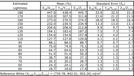
in the SL1>100 experiment.) The mean visual data and their estimated standard error of the mean,

calculated by the Equation (2.7), are listed in the Table 2.2.

Table 2.2: Visual data of the lightness scaling experiments, SL1>100 and SL1<100

For the range between mid-gray and white (L=100), the uncertainty of the 1933’s visual data is

between 0.8 and 1.3, as shown in section 2.3.1, and the uncertainty of the SL1<100 experiment is

between 0.7 and 1.5. It seems the two experiments are comparable. However, there are two questions

raised. First, the uncertainty of the 1933’s data is in ascending order, but the uncertainty of the SL1<100

Estimated Mean (%) Standard Error (Se)

Lightness X10/Xn,10 Y10/Yn,10 Z10/Zn,10 X10/Xn,10 Y10/Yn,10 Z10/Zn,10

180 447.0 438.4 445.7 33.9 32.5 33.3

170 310.9 307.5 311.8 21.6 21.2 21.0

160 273.0 270.5 274.5 18.9 18.5 18.4

150 232.0 230.5 234.9 13.3 13.0 13.1

140 209.6 208.6 212.8 9.9 9.7 9.8

130 184.1 183.6 187.2 7.5 7.3 7.4

120 154.6 154.8 157.8 4.2 4.2 4.3

110 127.7 127.8 129.8 2.1 2.1 2.2

95 88.1 88.0 88.7 0.7 0.7 0.7

90 75.0 74.9 75.1 1.0 1.0 1.1

85 64.7 64.6 63.7 1.0 1.0 1.1

80 51.5 51.4 50.2 1.2 1.2 1.2

75 38.7 38.6 37.1 1.3 1.3 1.3

70 30.3 30.2 28.7 1.3 1.3 1.3

65 24.3 24.1 22.7 1.5 1.5 1.5

60 18.7 18.6 17.4 1.5 1.5 1.4

is in descending order. Second, it is expected to have a lower uncertainty for a larger number of

observers, but the effect of the larger number of observers (50 here vs. 14 in the 1933’s) is not clear.

The questions might be mainly due to the experimental design. In the 1933’s partition scaling

experiment, all the selected intervals were presented together to increase the precision. For the SL1

experiments, there were only two stimuli presented to help observes to find the target interval, which

means much less anchor references. Recalling that it is difficult for observers to select the midpoint in

sensation between two stimuli that differ greatly, as the difference between two stimuli increases, the

difficulty increases. This can cause the descending order of uncertainties of the SL1<100, i.e., the

difficulty and uncertainty of finding “midpoint (L=60) between L*=100 and L*=20” is higher than

finding “midpoint (L=95) between L*=100 and L*=90”. This factor can also weaken or eliminate the

improvement of uncertainty from increasing the observer number.

For the range above white, the uncertainty is huge, 2.1 to 32.5. Several factors can be contributed to

this problem. First, similar to the difficulty of selecting midpoint between two stimuli that differ greatly

in sensation, it is also difficult to make the selection of the SL1>100 when the stimuli differ greatly.

Second, the initial stimulus of the adjusted sample was set as L=100, not the selected value in the

previous step. Hence, it is possible that the observer didn’t make an ordered selection, e.g., his/her

selection of L=150 could be lighter than L=160. This problem is shown in Figure 2.9, where all visual

data of 50 observers are presented. It is found that several observers didn’t have an ordered selection.

Third, as the magnitude of stimulus increase, the standard error will increase, as shown in the case of the

1933’s visual data. These should be the main factors to cause high uncertainty of the SL1>100

experiment. It should be noted that the first and second factors can be diminished when all the selections

are presented together in an order, such as what Munsell et al. [Munsell, 1933] did for the 1933 partition

Figure 2.9: The visual data of all 50 observers for SL1 experiments

For each estimated lightness value, the luminance values adjusted by observers in the experiments

are averaged. The estimated lightness values are then plotted as a function of the averaged luminance

and shown in Figure 2.10, with a gain-gamma (GG) model and a gain-gamma-offset (GGO) model

fitting functions optimized to roughly describe the visual data. Two functions are shown in Equation

(2.8) and (2.9), respectively. Error bars in Figure 2.10 are 95% confidence intervals based on the

standard errors of the mean estimates, as shown in Equation (2.10).

!

L_SL1,GG =105.12"(Y/Y_n)0.3847 (2.8)

!

L_SL1,GGO=79.13"(Y/Y_n)0.497

+24 (2.9)

Lower limit=x "Se#tCL

Upper limit=x +Se#tCL

where

!

x indicates the sample mean,

!

Se indicates the estimated standard error of the mean , and

!

tCL is

the t-score of the desired confidence level. The

!

tCL value for the 95% interval for degree of freedom 49

(df = N-1 = 50-1) is 2.0096.

Figure 2.10: The visual data, optimized lightness scale, and CIELAB lightness function.

The R-squared values of the GG and GGO model fittings are 0.986 and 0.988, respectively, optimized

with initial settings as a simple square-root function using Matlab. The GGO model includes an offset

term to describe the flare in the environment. Although it doesn’t exhibit an intersection with the origin,

it is closer to the real world, such as the flare in the environment. Other optimized functions based on

models with various offset terms [Katoh, 2001] have slightly better performance, but they either lack of

a term to describe the flare (gain-offset-gamma models, GOG) or accompany extreme large coefficients

It should be noted that fitting any model to describe the visual data is premature in this stage. For

example, although the GGO model provides better R-square value for fitting the visual data, its lightness

value for zero reflectance is a bad estimation, 24. More visual data, particularly in the range below a

lightness value of 60 with similar experimental setups, is required to correct and further refine a

wider-range lightness function.

The CIELAB lightness function is shown in Figure 2.10 as well, since that applies best for visual

data on a medium-gray background. There was a doubt whether the lightness scale exceeding diffuse

white will keep following the power-law or become flattened very quickly. Figure 2.10 shows that

response compression continues for the tested range and a power-based function can approximately

describe the results. The CIELAB lightness function follows the data qualitatively, but falls outside the

error bars for some parts of the range. This indicates that, in some extent, the calculated L* with values

larger than 100 are meaningful.

Experiment for 2-degree visual field (SL2<100 and SL2>100)

In the experiment of “SL1>100”, several observers reported that their reference whites were shifted,

to some degree, toward the stimulus brighter than white, when the presented sample patches were

brighter than the white background. To better control observer’s adaptation point, the sample patches in

the experiments for 2-degree visual field were smaller. The observers, participating in both the 2-degree

and 10-degree visual field experiments, reported that this configuration could help them to better

perceive the background and surround white as reference white.

The same group of 17 color-normal observers participated in the SL2<100 and SL2>100

experiments, where 15 of them were also observers in the first two experiments, SL1>100 and SL1<100.

The total range of estimated lightness values is from 0 to 200 at an interval of 12.5, and the mean visual

Table 2.3: Mean visual data of the lightness scaling experiments, SL2>100 and SL2<100

For the range below white (L=100), the uncertainty is between 0.7 and 2.9 for the SL2<100, between

0.2 and 1.3 for the 1933’s visual data (see section 2.3.1), and between 0.7 and 1.5 for the SL1<100 (only

from mid-gray to white). The uncertainty of the SL2<100 is larger than the SL1<100, and it might be

due to fewer observers in the SL2 experiments. However, there was a similar number of observers

between predicating in the SL2 and the 1933’s experiments (17 vs. 14), there should be other factors

contributing to the high uncertainty. One possible factor is that, in the 1933 experiment, it was very easy

for observers to re-adjust their selections to achieve an equal-interval scale. The observers only had to

move the stripes to quickly find the desirable selections. In the SL2<100, the observers had to use the

vacuum pen to slowly pick/remove their selections. Although they were encouraged to make necessary

adjustments, most of them stuck with their first selections. The design of putting all selected intervals

Estimated Mean (%) Standard Error (Se)

Lightness X2/Xn,2 Y2/Yn,2 Z2/Zn,2 X2/Xn,2 Y2/Yn,2 Z2/Zn,2

200.0 716.0 745.4 699.1 127.3 133.2 125.6

187.5 445.9 461.5 448.5 73.3 75.9 76.1

175.0 356.8 369.6 353.4 62.0 64.4 61.2

162.5 302.9 313.4 296.7 59.2 61.1 55.6

150.0 248.3 257.1 244.9 42.4 44.7 39.9

137.5 172.6 178.0 171.1 17.6 18.5 17.4

125.0 145.5 149.4 144.3 15.9 16.5 15.7

112.5 111.1 113.6 110.2 5.6 5.8 5.7

100.0 100.0 100.0 100.0 0.0 0.0 0.0

87.5 85.9 85.8 86.0 1.5 1.5 1.5

75.0 65.6 65.6 65.7 2.9 2.9 2.9

62.5 45.5 45.4 45.9 2.2 2.2 2.1

50.0 30.7 30.6 31.5 2.0 2.0 2.0

37.5 20.9 20.8 21.7 1.6 1.6 1.7

25.0 12.9 12.8 13.3 1.2 1.2 1.2

12.5 6.1 6.0 6.2 0.7 0.7 0.7

0.0 0.0 0.0 0.0 0.0 0.0 0.0

together in the SL2<100 provides the opportunity to achieve lower uncertainty than the SL1<100, but

this advantage could be eliminated by the difficulty of adjusting selections.

For the range above white, the uncertainty is from 5.8 to 133.2, which is huger than that of the

SL1>100. The same factors contributing to the large uncertainties of the SL>100 also affect the

SL2>100 experiment, such as the difficulty of making bisection selection when stimuli differ greatly in

sensation and the possibility of deriving a disordered scale. The individual responses of 17 observers are

shown in Figure 2.11, where several responses are disordered. Regarding the higher uncertainty than

that of the SL1>100, lesser observers could be one of the factors. Besides, in the SL1>100, standard

lightness samples were presented for selecting the samples brighter than white, but, in the SL2>100,

individual lightness samples were used instead. For example, to find the lightness 150, the same L*=50

sample was presented for the SL1>100 and different Li=50 samples were used for the SL2>100. This

Figure 2.11: The visual data of all 17 observers for SL2 experiments

For each estimated lightness value, the luminance values adjusted by observers in the experiments

are averaged. The estimated lightness values are then plotted as a function of the averaged luminance

and shown in Figure 2.12, with a GG model and a GOGO model fittings shown in Equation (2.11) and

(2.12), respectively, to roughly fit the visual data. Error bars in the figure are 95% confidence intervals

based on the standard errors of the mean estimates, as shown in Equation (2.10). The

!

tCL value for the

95% interval for degree of freedom 16 (df = N-1 = 17-1) is 2.1199.

!

L_SL2,GG =95.86"(Y/Y_n)0.4247 (2.11)

!

L_SL2,GOGO =101.29"(Y/Y_n#0.067)0.3837

Figure 2.12: The visual data, optimized lightness scales, and CIELAB lightness function.

The GG model is presented due to its simplicity. The GOGO model provides higher R-squared value

among those GG, GGO, GOG, and GOGO models, but the difference is not obvious either

quantitatively or graphically. (Models are optimized with initial settings identical to a simple square-root

function using Matlab.) There is a clear crispening effect around the white-point lightness, which is the

lightness of the background. It should have a better fitting by optimizing a Takasaki or Semmelroth –

type function. However, the crispening effect will not be significant in a complex configuration, which

is the case of most images. Besides, slight differences in the experimental design can cause significant

differences in the degree of crispening [Berns, 2000b; Cui, 2002], Therefore, fitting a lightness function

describing the crispening effect of SL2 visual data might not be suitable for applications in the printing

The projectors used in both SL1 and SL2 experiments were not perfectly gray balanced, but the

variation of a* and b* values were mainly within ±2 units. Further researches should be done with a

better gray-balance setting. That is because lightness depends on not only luminance but also

chromaticity, which is the related-color case for the Helmholtz-Kohlrausch effect [Fairchild, 2005a].

2.6 Conclusions

The visual data suggest that there is no significant difference between SL1 and SL2 experiments.

The visual data also show a clear crispening effect around the white-point lightness. The compressive

shape of lightness perception as a function of luminance factor can be approximately described by a

power-law-based function. This compressive shape has been shown to hold for a range exceeding

diffuse white with the psychophysical experiments described in this thesis. Optimized lightness function

and lightness weighting functions were derived to fit the visual data in a descriptive sense. The

optimized lightness function mainly corrects the under-prediction of the CIELAB lightness function for

the range exceeding diffuse white. More visual data are necessary to verify and improve the functions

and more fully specify lightness and color appearance outside the range of normal, diffuse, reflecting

3. SCALING LIGHTNESS DIFFERENCE ABOVE AND BELOW DIFFUSE WHITE

3.1 Introduction

Two psychophysical methods, constant stimuli [e.g., Berns, 1996] and gray-scale comparison [e.g.,

Luo, 1986], are frequently used for scaling differences of visual perception. In the method of constant

stimuli, observers are asked to judge whether the lightness difference of the anchor pair is greater or less

than the lightness difference of the test pair. This method is also referred to as pass-fail judgement. In

the method of gray-scale comparison, observers are asked to identify the lightness difference from a

lightness difference gray-scale with equal #E*ab lightness difference steps that is closest to the lightness difference of a test pair. The method of constant stimuli is preferable, because its technique is based on

fewer assumptions and provides marginally better precision [Montag, 2003]. Moreover, the method of

constant stimuli is easier for observers to make judgments and for the experimenter to analyze results.

3.2 Method of Constant Stimuli

Five to seven samples are usually created along the #L* direction for selected color centers to conduct lightness difference scaling using the constant stimuli method. A pilot experiment is typically

executed to estimate the approximate tolerance threshold. Then, samples are created around the

approximate tolerance threshold. The vector of each direction can be confirmed with principal

component analysis [Alman, 1989].

After conducting the visual judgement experiment, the responses of an individual observer, encoded

in 0 for smaller and 1 for larger than the lightness difference of the anchor pair, are corrected with a

3-by-1 low-pass filter (LPF) algorithm [Berns, 1991]. This LPF is based on the assumptions that, first, the

that of sample pairs in each group would tend to be chosen as smaller than that of the anchor pair, and

vice versa. An example of this algorithm is shown in Figure 3.1 adapted from Berns [1991].

Figure 3.1: An example for applying the 3-by-1 low-pass filter algorithm to correct the non-monotonic responses.

Probit analysis [Finney, 1971] is then applied to the filtered responses. By using Probit analysis, the

assumption that the responses follow a cumulative normal distribution is made. This assumption can be

tested and generally holds well for such experiments [Silberstein, 1945; Brown, 1952]. The percentage,

P, of the cumulative distribution at a specific color difference intensity, #E, can be described with Equation (3.1).

!

P= 1

" 2# exp

$1 2

%E$µ

" _d%E $&

%E

'

where µ and $ are the mean and standard deviation, respectively, to characterize a normal distribution curve.

The sigmoidal curve of the cumulative responses can be transformed into Probits (probability unit,

Z) and fitted with a probit model by regression. The Probit is defined as standard normal deviate

!

Z=5+"E#µ

$ (3.2)

!

Z ="+#$E (3.3)

The linear parameters % and & are derived by fitting all the responses, usually from 5 to 7 samples, via maximum likelihood technique. For a 50% probability of rejection (fail), Z equals to zero and m, in

Equation (3.4), represents the median color-difference tolerance, T50.

!

m="#

$ (3.4)

This calculation can be done with Matlab function “glmfit (

!

"E, [ r, n], ‘binomial’, ‘link’, ‘probit’)”,

where r is the responses and n is the number of observers.

The chi-squared value, calculated using Equation (3.5), is used to determine how well each set of

responses agrees with the Probit model.

!

"2= (r#nP)

2

nP(1#P)

$

where P is the predicted probability converted from the predicted Z score. When the calculated

!

"2 is

greater than a chi-squared value for the number of samples minus two degrees of freedom and a

significance of 10%, there is a significant difference between the data and the model. The difference can

be attributed to random factors in the experiment and can be corrected with a heterogeneity factor, h, as

given in Equation (3.6).

!

h= "

2

k#2 (3.6)

where k is the number of sample pairs, and h equals 1 when the Probit model well describes the

responses.

!

FL=m+ g

1"g

(

)

#(1"g) 1"g

Snw

+(m"x ) 2

Sxx

(3.7)

where

!

g= ht 2

"2S_xx (3.7a)

!

x = Snwx Snw

(3.7b)

!

w= Z

2

P(1"P) (3.7c)

!

Snw =

"

!

Snwx =

"

!

S_nwxx =

_"

!

S_xx =S_nwxx" Snwx

2

S_nw (3.7g)

For centers with insignificant chi-square values, the t value equals 1.96 at 95% confidence with

infinite degree of freedom; otherwise the t value is determined with (k-2) degrees of freedom.

Additionally, the standard error can be calculated with the upper fiducial limit (UFL), lower fiducial

limit (LFL), and T50 using Equation (3.8).

!

SE =UFL"LFL

2#T50 (3.8)

When the chi-squared value is larger than the criterion or the color differences of samples do not

vary along a vector quite well, such as when the first eigenvalue is smaller than 0.99, the 3D Normit

analysis [Berns, 1997] can be applied instead of Probit analysis. As variations in other two dimensions,

analysis, but the color difference values,

!

"E, should be replaced with the lightness difference values,

!

"L*.

The CIELAB values for color centers, +T50s, and -T50s are calculated for the evaluation and

development of color difference equations. The CIELAB values of color centers are the averaged values

for all the samples along the vector. The first eigenvector,

!

("L*_,

"a*_,

"b*₎

1stEigVec, of the group of samples

is used to calculate the CIELAB values of +T50 and -T50 according to Equation (3.9).

!

(L*,a*,b*)±T50=

(L*

,a*

,b*

)ColorCenter±T50"(#L *

,#a*

,#b*

)1stEigVec

(3.9)

3.3 Lightness Weighting Functions

Ideally, the lightness tolerances (T50s) should be identical at any position of the lightness scale when

the lightness scale is perceptually uniform. However, this is not the case for the CIELAB lightness

function. All the factors that affect lightness perception lead to this nonuniformity. One of the significant

factors is the crispening effect. Due to this effect, the minimum lightness tolerance corresponds to the

experimental background lightness [Berns, 2000b]. Slight differences in the experimental design can

cause significant differences in the degree of crispening [Berns, 2000b; Cui, 2002], which represents as

the degree of curvature in the plot of lightness tolerance against lightness position. When the curvature

is slight, this effect can be ignored, such as the lightness weighting function in CIE94 [Berns, 1993].

When the curvature is noticeable, a curve of U or V shape could be used to fit the visual data [Berns,

2000b; Luo, 2001; Chou, 2001]. The lightness weighting function of CIEDE2000 [Luo, 2001; Chou,

2001] exhibits this behavior and is shown in Equation (3.10).

S_{L, "E}

00 =1+

0.015(L*#50)2 20+(L*

It should be noted that the minimum weighting of the function is at the position of L* = 50, which is the

lightness value of the background suggested by CIE.

3.4 Experimental Designs

3.4.1 New experiments for a range both above and below diffuse white, DE>100

The method of constant stimuli was used in both experiments on lightness difference perception,

DE>100 and DE<100. The stimulus configuration of DE>100 is illustrated in Figure 3.2.

Figure 3.2: The configuration of lightness difference scaling experiment (DE>100). (The gray background and gray scales are printed, and the stimuli of two lightness difference

pairs are illuminated by the DLP on the paper white.)

generated by the DLP projections on the paper white. The size of each pair is 2-by-5-inches for a

viewing angle of about 4.8 degree at the distance of 24 inches. There were projected one-pixel black

frames for the samples and a projected one-pixel black dividing line between each pair. The L* value of

the background was 50. It should be noted that a diffuse white is used for CIELAB calculation in both

DE>100 and DE<100 experiments to correlate the results from the two sets of experiments. The

configuration is not a CIE reference condition for color difference experiments. The goal of this design

was to help observers have more information about the illuminant and preserve adaptation to the diffuse

white while presenting significantly lighter stimuli.

Nine lightness centers were chosen, where five were above, one near, and three below diffuse white.

The range of the nine lightness centers was from L*= 68 to L*=183. A pilot experiment was executed to

estimate the approximate tolerance threshold for each lightness center. Then, seven sample pairs were

created with differences of roughly 5/8, 6/8, 7/8, 8/8, 9/8, 10/8, and 11/8 of each approximate tolerance

threshold, mainly along the L* direction for each lightness center. PCA was applied to analyze each set

of fourteen patches for each lightness center. The first eigenvalues were greater than 0.99 cumulative

variance for the samples of all lightness centers. This establishes the uni-dimensionality of the stimuli.

The CIELAB values of the anchor pair were (L*,a*,b*) = (48.7, 0.2, 1.3) and (46.2, 0.2, 1.3), with a

#E*ab of 2.53. Smaller #E*ab values (1 and 2) had been tested as the anchor pair, but the differences were not as distinguishable as hardcopy samples with the same #E*ab values. This might be caused by the flickering and noisy projections. Sixty-three sample pairs were presented with different random

orders for each observer. The first ten samples presented, including six repeated testing pairs, were

always darker than the paper white. Observers were asked to choose the pair with larger lightness