Efficient block preconditioning for a C1 finite element discretisation of the Dirichlet biharmonic problem

CI. OMPUT c

Vol. 38, No. 1, pp. A325–A345 of the Creative Commons 4.0 license

EFFICIENT BLOCK PRECONDITIONING FOR A C1 FINITE

ELEMENT DISCRETIZATION OF THE DIRICHLET BIHARMONIC

PROBLEM∗

J. PESTANA†, R. MUDDLE†, M. HEIL†, F. TISSEUR†, ANDM. MIHAJLOVI ´C‡

Abstract. We present an efficient block preconditioner for the two-dimensional biharmonic Dirichlet problem discretized byC1_{bicubic Hermite finite elements. In this formulation each node} in the mesh has four different degrees of freedom (DOFs). Grouping DOFs of the same type together leads to a natural blocking of the Galerkin coefficient matrix. Based on this block structure, we develop two preconditioners: a 2×2 block diagonal (BD) preconditioner and a block bordered diagonal (BBD) preconditioner. We prove mesh-independent bounds for the spectra of the BD-preconditioned Galerkin matrix under certain conditions. The eigenvalue analysis is based on the fact that the proposed preconditioner, like the coefficient matrix itself, is symmetric positive definite (SPD) and assembled from element matrices. We demonstrate the effectiveness of an inexact version of the BBD preconditioner, which exhibits near-optimal scaling in terms of computational cost with respect to the discrete problem size. Finally, we study robustness of this preconditioner with respect to element stretching, domain distortion, and nonconvex domains.

Key words. biharmonic equation, Hermite bicubic finite elements, block preconditioning, con-jugate gradient method, algebraic multigrid

AMS subject classifications.65F08, 65F10, 65N22

DOI.10.1137/15M1014887

1. Introduction. The biharmonic operator is a key component in mathematical

models of a number of important physical problems. It arises in plane strain and plane stress elasticity problems, where the solution is expressed in terms of an Airy stress function (see [32, p. 79], [37, p. 288]) and in plate bending problems. It also occurs in the stream-function-vorticity formulation of two-dimensional Stokes flow [27].

The strong formulation of the Dirichlet biharmonic problem seeks the function

u∈C4(Ω) that satisfies

(1.1) ∇4u=f

in the domain (x₁, x₂) ∈ Ω ⊂ R2 with piecewise smooth boundary ∂Ω and source function f ∈L₂(Ω) subject to the Dirichlet boundary conditions

(1.2) u=g₁, ∂u

∂nˆ =g2 on ∂Ω,

where ∂u_∂ˆn denotes the outward normal derivative and g₁ and g₂ are given functions. In the context of the plate bending problem, the caseg₁ =g₂ = 0 corresponds to a clamped boundary.

∗_{Submitted to the journal’s Methods and Algorithms for Scientific Computing section March 31,}

2015; accepted for publication (in revised form) November 10, 2015; published electronically January 28, 2016.

http://www.siam.org/journals/sisc/38-1/M101488.html

†_{School of Mathematics, The University of Manchester, Manchester M13 9PL, UK (jennifer.}

[email protected], [email protected], [email protected], francoise. [email protected]). The work of the first and fourth authors was supported by Engineering and Physical Sciences Research Council grant EP/I005293. The fourth author was also supported by a Royal Society-Wolfson Research Merit Award.

‡_{School of Computer Science, The University of Manchester, Manchester M13 9PL, UK (milan.}

[email protected]).

Numerical schemes for solving (1.1)–(1.2) either approach the problem directly or reformulate it as a mixed formulation (i.e., solve a system of two second-order problems). The advantages of using the former approach include better asymptotic accuracy for the same level of grid resolution (see [1, Thm. 5.4], [10, Thms. 6.1.6 and 7.1.6 and p. 392]) and a symmetric positive definite (SPD) coefficient matrix for the discrete problem. Conversely, for the mixed formulation, discretization (by a finite difference or finite element method, for example) results in a linear algebraic system that is symmetric but indefinite.

In this paper we consider a conformingC1 finite element approach [26], for which the standard weak form is to findu∈H2(Ω) satisfying (1.2) such that

(1.3)

Ω∇

2_u∇2_{v dΩ =} Ω

f v dΩ

holds for all test functions v ∈ H₀2(Ω), where H₀2(Ω) = {v ∈ H2(Ω)|v = _∂∂v_nˆ = 0 on∂Ω}. The discrete weak formulation is obtained by restricting (1.3) to a finite-dimensional space S(Ω) ⊂ H2(Ω), for which we adopt a basis associated with the bicubic Hermite (Bogner–Fox–Schmit) finite elements [6, p. 72]; these are formed from a tensor product of one-dimensional Hermite polynomials. The C1 continuity across element boundaries is ensured by assigning four degrees of freedom (DOFs) to each node, corresponding to four different basis functions.

The finite element approximation of (1.3) is then obtained by solving a linear systemAx=b, whereA ∈ RN×N is a large, sparse, and SPD matrix andb∈RN. Such systems are usually solved by iterative methods, with the conjugate gradient (CG) method a popular choice [16, Chap. 2]. Grouping together the unknowns corre-sponding to the same DOF type leads to the following natural 4×4 blocking of the coefficient matrix:

(1.4) A=

⎡ ⎢ ⎢ ⎣

A₁₁ A₁₂ A₁₃ A₁₄ AT₁₂ A₂₂ A₂₃ A₂₄ AT₁₃ AT₂₃ A₃₃ A₃₄ AT₁₄ AT₂₄ AT₃₄ A₄₄

⎤ ⎥ ⎥ ⎦,

where A_ij ∈ Rn×n, i, j = 1, . . . ,4, and N = 4n, where n is the number of interior nodes. Since the biharmonic operator is fourth order, the two-norm condition number of the matrixAbehaves asκ(A) =O(h−4), wherehis the mesh parameter (assuming uniform discretization), and we find that mesh refinement generally has a detrimental effect on the convergence speed of the CG method. This problem can be rectified by effective preconditioning.

There are a number of preconditioning strategies for conformingC1discretizations of (1.1)–(1.2). The proposed methods include additive Schwarz methods [15], [40], [41], Bramble–Pasciak–Xu (BPX) preconditioning [26], Steklov–Poincar´e operator-based preconditioning [23], problem-specific multigrid methods [7], [9], [19], [33], [38], and fast auxiliary space preconditioning (FASP) [39].

Block preconditioners with multigrid components have also been considered. Aksoylu and Yeter [2] develop preconditioners with blocks based on regions of high and low bending, while Bjørstad [3] uses blocks arising from a separation of variables of a related problem. Peisker and Braess [29] use a blocking based on basis func-tion types, as we do, but their precondifunc-tioner is based on a mixed formulafunc-tion of the biharmonic problem. Other preconditioners for the mixed formulation use blocks associated with different differential operators, and efficient preconditioners of this

sort apply multigrid to the Dirichlet Laplacian blocks [31] or the Schur complement system [17].

In this paper we propose two novel preconditioners that are fully algebraic and assembled from the element matrices in a manner analogous to the matrixA, making them easy to implement. The first of these is a 2×2 block diagonal (BD) precon-ditioner. The positive definiteness of Aand the assembly of the preconditioner from element matrices mean that analysis based on the general ideas of Wathen [34], [35], [36] can be applied to demonstrate that mesh-independent convergence is guaranteed in certain cases.

The second preconditioner introduced in this paper is a computationally cheaper block bordered diagonal (BBD) approximation of the block diagonal preconditioner that is feasible for larger problems and can be implemented in a cost-effective manner. For this second preconditioner we provide some spectral analysis. We then employ numerical experiments to demonstrate mesh-independent convergence rates and show that it is possible to deploy off-the-shelf multigrid approximations for certain matrix blocks.

The paper is organized as follows. In section2we discuss the finite element assem-bly process of the matrixAin (1.4) and relevant aspects of the CG method. Section3

describes the new block diagonal preconditioner. We characterize the eigenvalues of the preconditioned matrix and give conditions for mesh-independent convergence. However, the preconditioner is costly to apply. We therefore introduce a more prac-tical block bordered diagonal preconditioner in section 4 and provide an eigenvalue analysis. We propose an inexact version of the BBD preconditioner, which involves matrix lumping and algebraic multigrid approximation. Finally, we present numerical experiments in section 5 that verify the effectiveness of the inexact BBD precondi-tioner, and we investigate its robustness with respect to changes in the domain and element shape.

2. Preliminaries. In this section we describe the details of the finite element

assembly process for the biharmonic problem and introduce the preconditioned con-jugate gradient (PCG) method.

2.1. The finite element assembly process. The analysis of the spectra of

the preconditioned matrices in later sections will be based on the fact that the finite element matrixAin (1.4) is assembled from element contributions. In this section we describe this assembly process.

We discretize (1.3) usingC1Hermite finite elements, defined in a reference domain with local coordinates (s₁, s₂) ∈ Ω = [−1,1]2. The solution within the element is represented as

u(s₁, s₂) =

4

j=1 4

k=1

U_jkψ¯_jk(s₁, s₂),

where U_jk are the unknown coefficients and ¯ψ_jk are the reference Hermitian basis functions. The subscript j represents the node number and k enumerates the DOF type such that at node j, U_jk interpolates u, _∂s∂u

1,

∂u ∂s2, and

∂2_u

∂s1∂s2 for k = 1, . . . ,4,

respectively. The same basis functions are used to isoparametrically map the reference element to the actual element Ω_e.

Consider now a finite element discretization of the domain Ω consisting of M

elements, and let A_e ∈ R16×16, e = 1, . . . , M, be the biharmonic element matrices

associated with these elements. The matricesA_e are symmetic positive semidefinite, and each entry is of the form

(A_e)_ij=

Ω∇ 2_ψ¯_i

1i2∇2ψ¯j1j2|Je|dΩ,

wherei= 4(i₂−1)+i₁,j= 4(j₂−1)+j₁, andJ_eis the element Jacobian. Consequently, multiplying A_e by a vector u ∈ R16, with elements u_j = u_j1j2, is equivalent to computing integrals of linear combinations of basis vectors, that is,

(A_eu)_i=

Ω∇ 2_ψ¯

i1i2 ⎛ ⎝ 4

j1,j2=1

∇2_u

j1j2ψ¯j1j2 ⎞_⎠

dΩ.

Thus, the nullspace vectors ofA_ecan be thought of in terms of linear combinations of certain basis functions. These nullspace basis functions are harmonic functions, i.e., functions for which the Laplacian is zero (see (1.3)). It is straightforward to verify that a basis for these harmonic functions is

(2.1) 1, s₁, s₂, s₁s₂, s2₁−s2₂, s₂(s2₁−s2₂/3), s₂(s2₁/3−s2₂), ands₁s₂(s2₁−s2₂),

from which the nullspace ofA_e can be computed.

Now let us describe the assembly process of (1.4) mathematically. We introduce the matrixL_e∈R16×N that maps the entries ofA_eto entries ofA. Then

(2.2) A=

M

i=1

LT_eA_eL_e=LTdiag(A_e)L∈RN×N,

where

(2.3) L=LT₁ LT₂ . . . LT_MT ∈R16M×N

and diag(A_e) is a block diagonal matrix of element matricesA_e,i = 1, . . . , M. The matrix diag(A_e) is related to the differential operator and the choice of basis functions, whileLprovides information about the geometry and boundary conditions.

During this assembly process, unknowns corresponding to the same DOF type are grouped together, and this leads to the natural blocking of the coefficient matrix as

(2.4) A=

⎡ ⎢ ⎢ ⎣

A₁₁ A₁₂ A₁₃ A₁₄ AT₁₂ A₂₂ A₂₃ A₂₄ AT₁₃ AT₂₃ A₃₃ A₃₄ AT₁₄ AT₂₄ AT₃₄ A₄₄

⎤ ⎥ ⎥ ⎦,

u ∂u ∂s1

∂u ∂s2

∂2_u

∂s1∂s2.

The unknown vectorxand the right-hand side bare blocked accordingly.

2.2. The conjugate gradient method. The CG method is perhaps the best

known Krylov subspace method for solving sparse linear systems, and it is suitable for systems with an SPD coefficient matrix. The relative error after k iterations of CG is bounded by [16, p. 51]

e(k) A e(0)_A ≤2

α(A)−1

α(A) + 1

k ,

Table 1

Extremal eigenvalues and two-norm condition number ofAfor uniform meshes as a function of the problem sizeN.

Elements 4×4 8×8 16×16 32×32 64×64

N 36 196 900 3844 15876

λmin 56.20 18.45 4.94 1.26 0.32 λmax 1287 5705 23399 94179 377295 κ(A) 23 309 4735 74912 1.20×106

where e(k) =x−x(k) and α(A) =λ_max(A)/λ_min(A). SinceA is SPD,α(A) corre-sponds to the two-norm condition number κ(A). As mentioned in the introduction and verified numerically in Table 1, κ(A) = O(h−4). Although this bound may be pessimistic, we do see a deterioration in convergence speed of the CG solver as the mesh is refined (see the computations in section5).

The effective condition number [4], [30]

κ_eff= b2

λ_min(A)x₂

can better describe the effect of perturbations ofAand the right-hand side bon the solutionx, but it does not describe the convergence rate of the CG method (which is determined by a complex interaction between the spectrum ofAand the right-hand side). Li, Huang, and Huang [24] have shown that for the biharmonic equation and Hermite elements, the effective condition number is O(h−3.5) for general problems but can be as low as O(1) for certain boundary conditions. We observe this O(1) behavior for the homogeneous Dirichlet biharmonic problem (1.1) with f = 1 when square, stretched, or deformed elements are used (see Figure3).

The problem of slow convergence rates can be alleviated by solving an equivalent preconditioned system P−12AP−12y =P−12bwith x =P−12y, whereP ∈ RN×N is SPD. Note that the CG algorithm itself requires only a linear system solve with P at each iteration; i.e., the matrix P−12 is never explicitly formed. The error of the preconditioned CG iterates can be bounded by

e(k)_A

e(0)_A ≤2

α(P−1A)−1

α(P−1A) + 1

k .

The error bound shows that the convergence of the CG method is accelerated when the condition number of the preconditioned matrixP−1Ais small. It can also be shown that fast convergence rates are achieved when the eigenvalues belong to a small number of tightly bounded clusters (see, for example, [16, sect. 3.1]). If the eigenvalues of P−1A can be bounded independently of the mesh size h (and possibly other problem parameters), thenP is an optimal preconditioner, in the sense of convergence of the CG method. If, in addition, linear systems involvingP can be solved in a manner that scales linearly with the problem size, then we have an optimal solver.

3. An ideal preconditioner. We first consider the block diagonal

precondi-tioner

(3.1) P_BD =

⎡ ⎢ ⎢ ⎣

A₁₁ A₁₂ A₁₃ AT₁₂ A₂₂ A₂₃ AT₁₃ AT₂₃ A₃₃

A₄₄

⎤ ⎥ ⎥ ⎦.

Since any principal submatrix of an SPD matrix A is itself SPD [21, p. 397], the preconditionerP_BD∈RN×N is also SPD. Additionally,P_BD is formed from a subset of the block matricesA_ij ofA,and so it is possible to assembleP_BD from the element matrix contributions in a manner analogous to that described in section2.1. Thus,

(3.2) P_BD=LTdiag(P_e)L,

where P_e is obtained from A_e, with values that would be assembled into A_i4 or AT_i4

set to zero fori= 1,2,3. The element contribution to the preconditioner (henceforth, the element preconditioner)P_e, likeA_e, is symmetric positive semidefinite, but it has rank 11 rather than 8. Straightforward computation shows that the nullspace ofP_e

is spanned by vectors corresponding to 1, s₁, s₂, s2₁−s2₂, and s3₁(2s₂−1) +s3₂(1− 2s₁) + 3s₁s₂(s₂−s₁). Note that the last of these functions is a combination of the last three functions in (2.1). Consequently, the nullspace of diag(P_e) is contained in the nullspace of diag(A_e) as stated in the following lemma, which will be relevant in the subsequent analysis.

Lemma 3.1. Let diag(P_e)be as in (3.2), and let diag(A_e)be as in (2.2). Then

null(P_e)⊂null(A_e)andnull(diag(P_e))⊂null(diag(A_e)).

We investigate analytically the spectral properties ofP_BD−1A. For convenience we introduce the notation

(3.3) A=

⎡ ⎢ ⎢ ⎣

A₁₁ A₁₂ A₁₃ A₁₄ AT₁₂ A₂₂ A₂₃ A₂₄ AT₁₃ AT₂₃ A₃₃ A₃₄ AT₁₄ AT₂₄ AT₃₄ A₄₄

⎤ ⎥ ⎥ ⎦=

A B

BT A₄₄

, P_BD =

A A₄₄

.

Then the eigenvalues ofP_BD−1Aare characterized by the following theorem.

Theorem 3.2. _{Assume that rank(B) =r in (3.3). Then} P−1

BDA ∈RN×N, with

AandP_BD given by (1.4)and (3.1), respectively, has N−2runit eigenvalues. The remaining2reigenvalues λsatisfy

0<1−√μ_max≤λ≤1 +√μ_max<2,

whereμ_max∈(0,1) is the largest eigenvalue of A₄₄−1BTA−1B.

Proof. SinceP_BD−1A is similar toP−12

BDAP−

1 2

BD, which is SPD, any eigenvalueλof

P−1

BDAis real and positive. Using (3.3), we see that λsatisfies

Au+Bv=λAu,

(3.4)

BTu+A44v=λA44v,

(3.5)

whereu∈R3n andv∈Rn are not simultaneously zero andN = 4n.

If λ= 1, then (3.4) implies that Bv =0, i.e., that v = 0or v ∈ null(B). We can find n−r linearly independent vectors in null(B) for which (3.4) and (3.5) are satisfied withu=0. Otherwise, v=0,and it follows from (3.5) that u∈null(BT). Since we can find 3n−r linearly independent vectors in null(BT), we have that one is an eigenvalue ofP_BD−1Awith multiplicity 4n−2r=N−2r.

If λ = 1, then (3.4) implies that (λ−1)−1A−1Bv = u, and substituting for u in (3.5) gives that

A−₄₄1BTA−1Bv= (λ−1)2v.

From this we see that nonunit eigenvaluesλofP_BD−1Aare given by λ= 1 +√μand

λ= 1−√μ, whereμis a nonzero eigenvalue ofA₄₄−1BTA−1B. Also, sinceAis positive definite, 0< μ <1 [21, Thm. 7.7.7]. The result follows.

The rank ofB is at mostn, so at least 2neigenvalues are equal to one, while the largest nonunit eigenvalue is less than two, regardless of the mesh size. The focus of the remainder of this section is to bound the smallest nonunit eigenvalue, since doing so ensures mesh-independent convergence.

To bound the smallest eigenvalue ofP_BD−1Awe adapt the analysis of Wathen [34], [35], [36] to our case. The basic idea is to determine the eigenvalues of the precon-ditioned element matrix diag(P_e)−1diag(A_e) and to then obtain mesh-independent bounds using Rayleigh quotients. In our case this approach is complicated by the fact that the singular matrices diag(A_e) and diag(P_e) have nullspaces of different di-mensions. However, we can still apply the general methodology since we know from Lemma3.1that null(diag(P_e))⊂null(diag(A_e))⊂R16M.

To deal with the different nullspaces involved it is useful to introduce certain subspaces ofR16M. Specifically, we define

(3.6) R:= range(diag(Ae)), Z:= null(diag(Ae)), N := null(diag(P_e)), M:=Z ∩ N⊥,

whereN⊥ is the space of all vectors orthogonal to vectors inN. With these spaces,

R16M _{=R+N +M, with N ⊂ Z. Furthermore, since the matrices diag(Ae) and}

diag(P_e) are BD, the basis vectors ofR,N,Z,andMcan be constructed from their element contributions.

In addition to the spaces defined above, we require the following lemma that shows that nonzero vectors inRN cannot be mapped to Z by the connectivity matrix.

Lemma 3.3. If x∈RN is a nonzero vector, then Lx∈ Z, where L, diag(A_e),

diag(P_e), andZ are defined by (2.3),(2.2),(3.2), and (3.6), respectively.

Proof. BothAandP_BD are positive definite, which implies that for anyx=0,

Ax=LTdiag(A_e)(Lx)= 0 and P_BDx=LTdiag(P_e)(Lx)= 0.

We know from Lemma3.1that null(diag(P_e))⊂null(diag(A_e)) =Z, soLx∈ Z. Both A and P_BD are positive definite, and so λ_min(P_BD−1A) has the variational characterization [28, Chaps. 1 and 15]

λ_min(P_BD−1A) = min

x=0

xT_Ax

xT_PBDx = min_y=Lx,

x=0

yT_diag(Ae)y

yT_diag(Pe)y.

Lety=y_R+y_M+y_N, wherey_R∈ R,y_N ∈ N, andy_M∈ MwithR,N, andM defined in (3.6). Lemma3.3shows thaty_R=0,and so

(3.7) λ_min(P_BD−1A) = min

y=yR+yM yR=0

yT

Rdiag(Ae)yR

(y_R+y_M)T diag(P_e)(y_R+y_M).

This appears problematic because, without any restriction on the size of y_M, the smallest eigenvalueλ_min(P_BD−1A) could asymptotically tend to zero. To prevent this, we must somehow bound the size of the denominator of (3.7). This is achieved by the next result, provided thatyT_Rdiag(P_e)y_R ≥δy_MT diag(P_e)y_M for some δ≥δ∗>0,

a condition that we verified numerically in Table4for the regular and stretched grids depicted in Figure1.

Lemma 3.4. _Let y_=Lx_,x∈RN_,x_{=0,be decomposed as}

(3.8) y=y_R+y_M+y_N,

where y_R ∈ R,y_N ∈ N, and y_M ∈ M with R, N, and M defined in (3.6). Addi-tionally, assume that

(3.9) yT_Rdiag(P_e)y_R≥δyT_Mdiag(P_e)y_M

for someδ≥δ∗>0. Then

(3.10) (y_R+y_M)Tdiag(P_e)(y_R+y_M)≤ζyT_Rdiag(P_e)y_R,

whereζ= 2 (1 + 1/δ).

Proof. From Lemma 3.3 we know that y_R = 0. Since diag(P_e) is symmetric positive semidefinite, it has a semidefinite square root, and there are vectorsa∈R16M andb∈R16M for which (y_R+y_M)Tdiag(P_e)(y_R+y_M) = (a+b)T(a+b).

Now, for any vectorsaand bof the same dimension,

0≤ a−b2₂= (a−b)T(a−b) = 2(aTa+bTb)−(a+b)T(a+b)

or (a+b)T(a+b)≤2(aTa+bTb). Thus,

(3.11) (y_R+y_M)Tdiag(P_e)(y_R+y_M)≤2(yT_Rdiag(P_e)y_R+yT_Mdiag(P_e)y_M).

Combining (3.11) with (3.9) gives (3.10).

We have been unable to prove that (3.9) holds for all meshes for the Dirichlet biharmonic problem, since it does not appear straightforward to remove the influence of the connectivity matrixL. However, there is strong numerical evidence to suggest that the assertion holds. In particular, letP_RandP_Mbe orthogonal projectors onto RandM, respectively. Then for any vectory=Lx,x=0,

yT

Rdiag(Pe)yR yT

Mdiag(Pe)yM = x

T_LT_PT

Rdiag(Pe)PRLx xT_LT_PT

Mdiag(Pe)PMLx≥

δ_min,

where

(3.12) δ_min=λ_min(LTP_MT diag(P_e)P_ML)−1(LTP_RTdiag(P_e)P_RL).

The value ofδ_minis tabulated for a sequence of uniformly refined meshes of square elements in Table2. From this we see that for square elements,δ_minappears to tend to 1.05, so that (3.9) is satisfied for uniformly refined meshes of square elements with

δ >1.05.

With these results in hand, we now bound the smallest eigenvalue of P_BD−1A. Under the assumption (3.9), we combine the decomposition (3.8) with Lemma3.4to give that, for anyy=Lx,x=0,

(3.13) y

T_diag(Ae)y

yT_diag(Pe)y =

yT

Rdiag(Ae)y_R

(y_R+y_M)Tdiag(P_e)(y_R+y_M) ≥ 1

ζ

yT

Rdiag(Ae)y_R

yT

Rdiag(Pe)yR

,

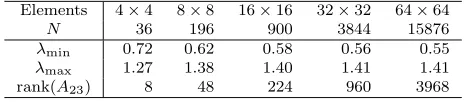
Table 2

Smallest (λmin) and largest (λmax) eigenvalues of the preconditioned operatorP_BD−1A,rank(B) from Theorem 3.2, andδmin from (3.12)for a sequence of uniformly refined grids and square ele-ments.

Elements 4×4 8×8 16×16 32×32 64×64

N 36 196 900 3844 15876

λmin 0.72 0.64 0.61 0.60 0.60 λmax 1.28 1.36 1.39 1.40 1.40 rank(B) 9 49 225 961 3969 δmin 1.17 1.06 1.05 1.05 1.05

where, by Lemma3.3,y_R=0. It follows from (3.7) that

(3.14) λ_min(P_BD−1A)≥θ

ζ, θ:= minyR∈R yR=0

yT

Rdiag(Ae)y_R

yT

Rdiag(Pe)y_R.

Since diag(P_e), diag(A_e),and the projectorP_RontoRare block diagonal, the above minimization over all nonzeroy_Rcan be carried out using individual element matrices. We computed the minimum for our element matrices and found thatθin (3.14) is larger than 0.046 for square elements. Sinceζ <3.91 for square domains and square elements, we have that λ_min(P_BD−1A) > 0.0118. Combining (3.9) with Theorem 3.2

gives the following bounds on the eigenvalues ofP_BD−1A.

Corollary 3.5. LetAandP_BDbe as in (1.4)and (3.1), and assume that (3.9) holds. Then for square domains and square elements, the eigenvalues λ of P_BD−1A satisfy 0.0118 < λ ≤ 2 and κ₂(P_BD−1A) < 170 independently of the mesh spacing parameterh.

Comparison with Table2shows that the bounds in Corollary3.5are pessimistic. However, combined with the high multiplicity of the unit eigenvalue, they show that we can expect fast convergence of preconditioned CG whenever (3.9) is satisfied.

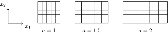
We also tested assumption (3.9) for rectangular domains using elements that are stretched in thex₁direction, withadenoting the ratio of the length of the horizontal side to the length of the vertical, as shown in Figure 1. We see from Table 3 that

δ_min decreases as the aspect ratio increases but that, for a fixed aspect ratio, δ_min

seems to tend to a constant as the mesh is refined. On the other hand, θ in (3.14) actually increases with a (see Table4). The net result is the eigenvalue bound θ/ζ

in Table 4 that slowly decreases as the aspect ratio increases but is asymptotically independent of the mesh width, and that qualitatively captures the behavior of the smallest eigenvalue.

x₁ x₂

a= 1 a= 1.5 a= 2

Fig. 1_{. Stretched elements. The domain is stretched in the}x1 _{direction and the deformation}

is described by the aspect ratioa.

4. A practical preconditioner. Although the preconditionerP_BDin (3.1) has

favorable spectral properties, it is prohibitively expensive to apply for large problems,

Table 3

Smallest (λmin) and largest (λmax) eigenvalues of the preconditioned operatorP_BD−1Aandδmin from(3.12)for stretched grids with different aspect ratiosa.

Elements 4×4 8×8 16×16 32×32 64×64

N 36 196 900 3844 15876

a= 1.5

λmin 0.62 0.52 0.50 0.49 0.49 λmax 1.38 1.48 1.5 1.51 1.51 δmin 0.85 0.59 0.52 0.51 0.50

a= 2

λmin 0.47 0.38 0.35 0.34 0.34 λmax 1.53 1.62 1.65 1.66 1.66 δmin 0.58 0.34 0.28 0.27 0.27

a= 2.5

λmin 0.36 0.27 0.25 0.24 0.24 λmax 1.64 1.73 1.75 1.76 1.76 δmin 0.41 0.22 0.18 0.17 0.16

Table 4

The values ofδ∗ andζin Lemma3.4,θ in (3.14), and the lower boundθ/ζ onλmin(P_BD−1A) for stretched elements with different aspect ratiosa.

a 1 1.5 2 2.5

δ∗ _{1.05 0.50 0.27 0.16}

ζ 3.9 6.0 9.5 14 θ 0.047 0.053 0.062 0.068 θ/ζ 0.011 0.008 0.006 0.004

since it requires the solution of linear subsystems involving the 3n×3nmatrixA. We will now investigate the block bordered diagonal (BBD) preconditioner

(4.1) P_BBD=

⎡ ⎢ ⎢ ⎣

A₁₁ A₁₂ A₁₃ AT₁₂ A₂₂

AT₁₃ A₃₃

A₄₄

⎤ ⎥ ⎥ ⎦

that is formed by omitting A₂₃ and AT₂₃ from P_BD. Unlike P_BD, the symmetric positive definiteness ofAis not enough to guarantee that P_BBD is positive definite. However, P_BBD was found to be positive definite in all the numerical experiments (performed with square, stretched, and deformed meshes) presented in section5below. Compared to the even simpler block Jacobi preconditioner

(4.2) P_J=

⎡ ⎢ ⎢ ⎣ A₁₁ A₂₂ A₃₃ A₄₄ ⎤ ⎥ ⎥ ⎦,

PBBD retains the coupling betweenuand both first derivative (_∂s∂u

1 and

∂u

∂s2) DOFs.

We will see in section 5 that this is essential to obtaining low and asymptotically constant iteration counts as the mesh is refined.

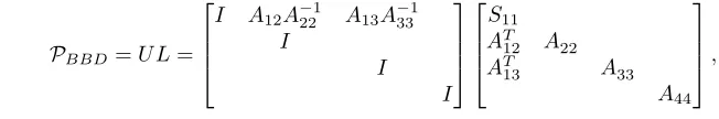
The action ofP_BBD−1 on a vector can be computed by means of the unsymmetric UL decomposition

(4.3) P_BBD=U L=

⎡ ⎢ ⎢ ⎣

I A₁₂A−₂₂1 A₁₃A−₃₃1 I I I ⎤ ⎥ ⎥ ⎦ ⎡ ⎢ ⎢ ⎣ S₁₁ AT₁₂ A₂₂

AT₁₃ A₃₃

A₄₄

⎤ ⎥ ⎥ ⎦,

where

(4.4) S₁₁=A₁₁−A₁₂A−₂₂1AT₁₂−A₁₃A−₃₃1AT₁₃.

Note that the solveUw=vcan be performed in a block parallel manner.

The remainder of this section is devoted to understanding the spectral properties ofP_BBD−1 Aand deriving an approximation that can be implemented in a cost-optimal manner.

4.1. Eigenvalue analysis. The block structure ofP_BBDand, in particular, the

indefiniteness of the element matrices used in its assembly prevent us from applying the previously introduced analysis to bound the spectrum of P_BBD−1 A. Instead, we consider the eigenvalues ofP_BBD−1 P_BD and then apply the bounds

(4.5)

λ_min(P_BBD−1 P_BD)λ_min(P_BD−1A)≤λ(P_BBD−1 A)≤λ_max(P_BBD−1 P_BD)λ_max(P_BD−1A),

which follow from the Courant–Fischer theorem [21, Thm. 4.2.11], in conjunction with the bounds in Corollary3.5. The eigenvalues ofP_BBD−1 P_BD are given in the following lemma.

Lemma 4.1. Let rank(A₂₃) = s. Then 1 is an eigenvalue of P−1

BBDPBD with multiplicity N−2s,while the remaining 2seigenvaluesη satisfy

(4.6) (G−F A−₁₁1FT)v=η(G−F A−₁₁1FT)v,

wherev=0,

(4.7) FT =A₁₂ A₁₃, G=

A₂₂ A₂₃ AT₂₃ A₃₃

, andG=

A₂₂ A₃₃

.

Proof. In the notation of (3.3),

PBBD = A _A

44

, A=

⎡

⎣AA11T₁₂ AA12₂₂ A13

AT₁₃ A₃₃

⎤ ⎦,

and

P−1

BBDPBD= A

−1_A

I_n

,

whereI_n is the identity matrix of dimensionn. This shows that 1 is an eigenvalue of P−1

BBDPBD with multiplicity at leastn.

To obtain the remaining 3neigenvalues, let us further partitionAandA as

A=

A₁₁ FT

F G

, A=

A₁₁ FT

F G

,

where F and G are as in (4.7). Then, the result is obtained by a straightforward extension of Theorem 3.1 of Dollar et al. [13] to the case of rank-deficientF, which we sketch for completeness.

The eigenvaluesη ofA−1Asatisfy

A11u+FTv=ηA11u+ηFTv,

(4.8)

Fu+Gv=ηFu+ηGv,

(4.9)

Table 5

Computed smallest (λmin) and largest (λmax) eigenvalues of the preconditioned operator P−1

BBDAas well asrank(A23)for a sequence of uniformly refined grids of square elements.

Elements 4×4 8×8 16×16 32×32 64×64

N 36 196 900 3844 15876

λmin 0.72 0.62 0.58 0.56 0.55 λmax 1.27 1.38 1.40 1.41 1.41 rank(A23) 8 48 224 960 3968

where u ∈ Rn and v ∈ R2n are not simultaneously zero. From (4.8) we see that either η = 1 or A11u+FTv = 0. If η = 1, then, letting v = [vT₁ vT₂]T with

v1,v2∈Rn, we find that there aren−slinearly independent vectorsv1∈null(A₂₃) for which (4.8) and (4.9) are satisfied with v₂ =u = 0. Similarly, there are n−s

linearly independent vectors v2 ∈ null(AT₂₃) for which (4.8) and (4.9) are satisfied withv₁ =u=0. Otherwise,v =0,and we can find nlinearly independent vectors

u=0. Combining these results shows thatη= 1 with multiplicity 3n−2s. Ifη= 1,

thenu=−A−₁₁1FTv, and substituting into (4.9) gives (4.6).

Similarly to Theorem 3.2we see thatλ= 1 is an eigenvalue ofP_BBD−1 P_BD with high multiplicity. However, we have been unable to bound the remaining 2s eigenval-ues. In spite of this, combining Lemma4.1 with Corollary3.5 and (4.5) shows that most of the eigenvalues ofP_BBD−1 Alie in a bounded interval.

Corollary 4.2. When square elements are used in a square domain and (3.9) is satisfied, at least N−2s eigenvalues of P_BBD−1 Alie in (0.0118,2). Any remaining eigenvalues lie in(0.0118η_min,2η_max), whereη_minandη_maxare the smallest and largest eigenvalues of the generalized eigenvalue problem (4.6).

Remark1. Analogous results hold for rectangular domains and stretched elements

if we replace 0.0118 in Corollary4.2 by the appropriate boundθ/ζ onλ_min(P_BD−1A) in Table4.

The extreme eigenvalues of P_BBD−1 A are given in Table 5 as a function of the problem size N. From this we see that these eigenvalues do not differ greatly from the extreme eigenvalues ofP_BD−1A(see Table2), and in practice little is lost in terms of the asymptotic convergence speed by using a more practical preconditioner. The numerical evidence in Table5suggests that the extreme eigenvalues ofP_BBD−1 Aappear to be bounded under mesh refinement, although we have been unable to prove this analytically.

4.2. Further simplifications. Although the block decomposition (4.3) allows

the efficient application of P_BBD, to achieve a preconditioner with optimal cost we require optimal solvers for linear systems involving the principal diagonal blocksS₁₁,

A₂₂,A₃₃, andA₄₄.

First, we consider spectrally equivalent approximations ofA₂₂, A₃₃, andA₄₄.

Lemma 4.3. Let

(4.10) L₂₂= lump(A₂₂), L₃₃= lump(A₃₃),

wherelump(H) ={h_ij} with

h_ij =

_n

k=1hik, i=j,

0, i=j.

Then for uniformly refined meshes of square elements, the eigenvalues of L−₂₂1A₂₂

and L−₃₃1A₃₃ are contained in [1/3,1], while the eigenvalues of diag(A₄₄)−1A₄₄ are contained in[0.43,1.24].

Proof. The matrices A₂₂, A₃₃, and A₄₄ are assembled from 4×4 submatrices

A(22)_e , A(33)_e , andA(44)_e of the element matrixA_e. Additionally, the approximations

L₂₂ andL₃₃ are assembled from lumped versions ofA_e(22) andA(33)_e , while diag(A₄₄) is assembled from the diagonal of A(44)_e . All six of these element matrices are SPD. As a result, we can use the approach of Wathen [34] to prove the result. (Recall that a similar result was used in section 3, where we had to deal with singular element matrices.)

Remark 2. _{This result is not surprising since the spectrum of A22 = A33}

re-sembles that of a scaled mass matrix, and for such matrices lumping often gives spectrally equivalent operators. In particular, for our problem, λ(A₂₂) = λ(A₃₃) ∼

O(h−4)λ(M), whereM is a mass matrix; for uniform grids, this can be verified using Fourier analysis, similarly to the approach in [14, section 1.6]. Additionally, on a uniform mesh all entries ofA₂₂ andA₃₃ are nonnegative.

Remark3. For the stretched grids used in the numerical experiments in section5

below, L₂₂, L₃₃, and diag(A₄₄) are still spectrally equivalent to A₂₂, A₃₃, andA₄₄. However, the spectral equivalence bounds deteriorate as the aspect ratio increases. For example, whena= 2.5,the eigenvalues ofL₂₂−1A₂₂ lie in [0.04,1], the eigenvalues ofL−₃₃1A₃₃lie in [0.21,1],and the eigenvalues of diag(A₄₄)−1A₄₄lie in [0.28,2.4]. Some off-diagonal elements of A₂₂ and A₃₃ were found to be negative even for an aspect ratio ofa= 1.5.

Using (4.3) and Lemma4.3, we approximateP_BBD by

(4.11) P_BBD=

⎡ ⎢ ⎢ ⎣

I A₁₂L−₂₂1 A₁₃L−₃₃1 I

I I

⎤ ⎥ ⎥ ⎦ ⎡ ⎢ ⎢ ⎣

S₁₁ AT₁₂ L₂₂

AT₁₃ L₃₃

diag(A₄₄)

⎤ ⎥ ⎥ ⎦,

where

(4.12) S₁₁=A₁₁−A₁₂L−₂₂1AT₁₂−A₁₃L−₃₃1AT₁₃.

The blockS₁₁in (4.12) is a sparse approximation of the Schur complementS₁₁from (4.4), owing to the diagonal approximations (4.10), and can be assembled cheaply.

To apply the preconditionerP_BBD within the preconditioned CG algorithm, we must solve systems with S₁₁, L₂₂, L₃₃, and diag(A₄₄). The last three matrices are diagonal, and hence trivial to invert. For systems with S₁₁, we consider two ap-proaches: an LU factorization, which yields an exact solution but is not computation-ally optimal, or two V(2,2)-cycles of classical algebraic multigrid (AMG) with point Gauss–Seidel smoothing and Ruge–St¨uben coarsening [25], which has optimal cost but leads to an inexact solution (cf. Table 7). Using these approximations for the Schur complement subsystem, we obtain the preconditioners P_BBD[LU] and P_BBD[AMG] in which the Schur complement subsidiary system is solved using an LU factorization and AMG, respectively. In Table6 we present the spectral properties of the precon-ditioned operators (P_BBD[LU])−1A and (P_BBD[AMG])−1A. These results suggest that the

spectrum of (P_BBD[LU])−1Ais bounded under mesh refinement, as we might expect from the spectral equivalence bounds in Lemma 4.3, although the eigenvalues are not as tightly clustered as those of P_BBD−1 A in Table 2. However, the smallest eigenvalue of (P_BBD[AMG])−1Adecreases with mesh refinement; that is, the AMG approximation is not spectrally equivalent toS₁₁.

Table 6

Smallest (λmin) and largest (λmax) eigenvalues of (P_BBD[LU])−1_{Aand (P}[AMG]

BBD )−1A for a

se-quence of uniformly refined grids. For the AMG solver we use the HSL routineMI 20 [5,22]. Note that we were unable to obtain the eigenvalues of the largestP_BBD[AMG]preconditioned matrix because of memory constraints.

Elements 4×4 8×8 16×16 32×32 64×64

N 36 196 900 3844 15876

P[LU]

BBD

−1

A _λmaxλmin 0.40_1.25 0.33_1.30 0.30_1.31 0.29_1.32 0.28_1.32

P[AMG]

BBD

−1

A _λmaxλmin 0.40_1.25 0.31_1.30 0.21_1.31 0.13_1.32 —_—

5. Numerical experiments. In this section we examine the effectiveness of

the preconditionersP_BD,P_BBD, andP_BBDat reducing the number of CG iterations and the computational time. Additionally, we investigate the robustness of their per-formance with respect to stretching of the finite elements as well as deformations and nonconvexity of the domain. Throughout, we choose the homogeneous Dirichlet boundary conditions g₁ = g₂ = 0 in (1.2). Our default domain is the unit square domain Ω = [0,1]2 discretized by a uniform grid of square elements. Although we note that for finite element problems the stopping criterion for CG should be tied to the discretization error, to demonstrate mesh independence we terminate the precon-ditioned CG method when the residual decreases in norm by six orders of magnitude, that is,r(k)₂≤10−6r(0)₂.

All AMG results in this section are obtained with two V(2,2)-cycles using Ruge– St¨uben coarsening and point Gauss–Seidel smoothing. We note that different AMG methods may give different results. However, our aim is to develop an effective pre-conditioner that is easy to implement, and so we choose off-the-shelf codes that gen-erally work well for finite element problems [5]. Thus, for the smaller experiments in Tables7and8we use the HSL code MI 20 [5,22] with default options, except that we change the coarsening criterionc failfrom 1 to 2 (and alter the number of V-cycles). For all other experiments we useHypre’sBoomerAMG[20].

We first compare preconditioned CG iterations for P_BD, P_BBD, P_BBD[LU], and

P_BBD[AMG] for smaller problems using MATLAB. For comparison, we also present iteration counts for the block Jacobi preconditioner (4.2) and AMG applied as a preconditioner to the entire block re-ordered matrix A from (1.4). We stress that preconditionersP_BBD in (4.3) and P_BBD in (4.11) are parallelizable, like the block Jacobi preconditionerP_J in (4.2), as discussed in section4. Since the problems con-sidered here are of relatively small dimension, in addition to measuring the norm of the residual we computed the relative errorx−x(k)_A/x_Ain the energy norm at termination, which we found to be uniformly smaller than 1.8×10−7. Computations were performed with different right-hand sidesb: we used the right-hand side from the finite element discretization of (1.1) for f = 1 and a random right-hand side b. Both choices result in similar behavior, which shows that the convergence does not depend on the regularity of the forcing term. Consequently, only results forf = 1 are presented.

The results are given in Table7, from which we see that without preconditioning, the number of CG iterations increases rapidly and appears to grow asO(h−2). The application of the AMG and block Jacobi preconditioners reduces the number of iter-ations somewhat, but convergence is still mesh dependent. This is not surprising since

Table 7

CG iteration counts for the unpreconditioned system, and preconditioned CG iterations counts for several different preconditioners: AMG applied to the whole matrixAin(1.4),P_J,P_BD,P_BBD, and the two inexact versionsP_BBD[LU]andP_BBD[AMG].

Elements 4×4 8×8 16×16 32×32 64×64 128×128

N 36 196 900 3844 15876 64516

Unpreconditioned 6 29 74 216 741 2741

AMG 3 9 27 82 272 864

PJ 6 19 51 113 232 480

PBD 3 9 10 11 11 11

PBBD 4 10 11 12 13 14

P[LU]

BBD 5 14 16 17 18 19

P[AMG]

BBD 8 14 18 24 33 46

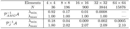
Table 8

Smallest (λmin) and largest (λmax) eigenvalues of the AMG and Jacobi preconditioned matrices.

Elements 4×4 8×8 16×16 32×32 64×64

N 36 196 900 3844 15876

P−1

AMGA _λmaxλmin 0.921.00 0.171.00 0.011.00 0.00081.00 ——

P−1

J A _λmaxλmin 0.181.80 0.042.02 0.0092.07 0.0022.09 0.00052.10

the condition numbers of these preconditioned matrices increase as the mesh is re-fined, as shown in Table8. (Note that we were unable to obtain the eigenvalues of the largest AMG preconditioned matrix because of memory constraints.) Conversely, the number of iterations required forP_BD,P_BBD, andP_BBD[LU] does not increase markedly with mesh refinement, and our experiments later in this section for larger problems indicate asymptotically mesh-independent convergence. This is in line with the spec-tral analysis in previous sections and the computed eigenvalues in Tables 2, 5, and

6.

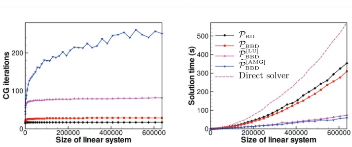
To explore the asymptotic behavior ofP_BBDfor larger problems, Figure2 shows the number of iterations required for convergence of preconditioned CG, and solu-tion times, for P_BD and the three block bordered diagonal preconditioners (P_BBD,

P_BBD[LU], and P_BBD[AMG]). These results were obtained using a C++ implementation in

oomph-lib [18] with SuperLU [12] for the direct solver. Note that times for the

unpreconditioned system, and for the block Jacobi and full AMG preconditioned systems, were similar to or larger than those of the direct method, and had poor asymptotic behavior. For this reason, timings for these preconditioners are not shown in Figure2.

We see from Figure2 that P_BD and P_BBD give mesh-independent convergence and that for both preconditioners the time to solution is lower than for the direct method. The use of P_BBD[LU] instead of P_BBD leads to a slight increase in iteration counts but mesh independence is retained. Furthermore, the solution times in Figure2

show that this increase in iterations is more than compensated for by the drastically reduced computational cost of applying the preconditioner. A further improvement can be achieved by replacing P_BBD[LU] by P_BBD[AMG]—Figure 2 shows that although the iteration count increases significantly, as expected from the eigenvalue computations in Table6, using AMG still reduces the solution times. This is due to the optimal cost of the AMG solver. Moreover, the solution times forP_BBD[LU] and P_BBD[AMG] scale approximately linearly with the problem size.

PBD PBBD

P[LU] BBD

P[AMG] BBD

Direct solver

Fig. 2_{. Number of preconditioned CG iterations (left) and solution times (in seconds). The}

execution time of the direct methodSuperLU_{applied to the system with coefficient matrix (1.4)is}

presented for comparison. The legend applies to both plots.

a

1

Stretched 1 1

b

Distorted Nonconvex

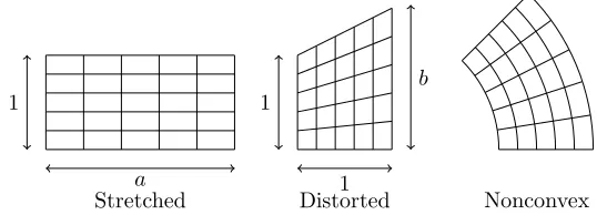
Fig. 3_{.Robustness tests. Stretched elements (left): the domain is stretched in the}x1_direction,

and the deformation is described by the aspect ratioa. Distorted domain and elements (middle): the top right corner is stretched upwards in thex2 direction with the ratio of the heights of the vertical boundaries parameterized byb. Curved nonconvex domain (right).

5.1. Robustness of the preconditioner. So far we have shown that the block

bordered diagonal preconditioners P_BBD[LU] and P_BBD[AMG] are nearly optimal in terms of wall clock time for a simple test problem. We will now evaluate the robustness of our preconditioners for problems with stretched grids and domains that are nonsquare and nonconvex. Stretched grids are needed, for example, for accurate computations of biharmonic eigenfunctions near the corners of the domain (see [8]). Figure3illustrates the following three tests considered:

1. Stretched elements. The domain is stretched in the x₁ direction, and the deformation is described by the aspect ratioa.

2. Distorted elements. The top right corner is stretched upwards in the x₂

direction; the ratio of the heights of the vertical boundaries is parameterized byb.

3. Curved domain. The rectangular domain is isoparametrically deformed to form a nonconvex curved domain.

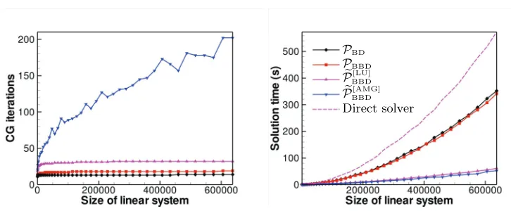
In all tests we used the same number of elements in each coordinate direction. We start by examining the effect of stretching the grid, as in the left of Figure3, on the preconditioners. The analysis in section3(forP_BD andP_BBD) suggests that an increase in the element aspect ratio is likely to have a detrimental effect on the effectiveness of the preconditioners. This is confirmed by Figure4 which shows the

PBD PBBD

P[LU] BBD

P[AMG] BBD

Direct solver

Fig. 4_{.Number of CG iterations (left) and solution time in seconds (right) for robustness test}

1(stretched elements) with aspect ratioa= 2.5. The execution time of the direct methodSuperLU

applied to the system with coefficient matrix (1.4)is presented for comparison. The legend applies to both plots.

iteration counts and solution times for a stretch ratio ofa= 2.5. Element stretching leads to a slight increase in the iteration counts and the solution times forP_BD and PBBD, although the asymptotic convergence rates obtained with these preconditioners remain mesh independent. As expected, the two inexact implementations of the BBD,

P_BBD[LU] andP_BBD[AMG], are affected more strongly. We attribute this to the fact that for sufficiently large stretch ratios, A₂₂ and A₃₃ have negative entries, which implies that the use of lumping and diagonal approximations in these preconditioners is less effective (cf. Remark3). P_BBD[AMG] is most sensitive because this preconditioner is also affected by the behavior of AMG on stretched meshes [11]. However, despite the noticeable increase in iteration counts, the plot of the solution times shows that the two inexact preconditioners remain significantly faster and scale better than the two exact preconditioners or the direct solver. In fact, over the range of problem sizes considered here,P_BBD[AMG] performs best.

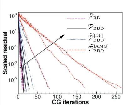
Figure5illustrates the effect of element stretching on the CG convergence histo-ries. For all four preconditioners, an increase in the element aspect ratio can be seen to lead to a decrease in the convergence rates (again consistent with the eigenvalue computations in sections3 and4). In all cases the norm of the scaled residual starts with a value of one but jumps to a much larger value during the first CG iteration. Subsequently, it decreases approximately linearly on a semilog scale as the CG iter-ation proceeds. This implies that a reduction in the CG convergence tolerance will result in a controlled increase in the number of iterations required to achieve a solution of the desired accuracy.

Figure6 shows the iteration counts and solution times for the deformed domain shown in the middle of Figure 3 (b = 1.5). In this case, P_BD, P_BBD, and P_BBD[LU] yield mesh-independent convergence rates, whereas the number of iterations obtained withP_BBD[AMG]appears to increase linearly with the problem size. WhileP_BBD[AMG]is still much faster than the exact preconditioners and the direct solver, P_BBD[LU] now yields the shortest execution times.

Finally, Figure 7 illustrates the performance of the preconditioners for the case of the curved, nonconvex domain shown in Figure 3. Here the trends are similar to those observed for the case of stretched grids. In particular, we observe

P

P

P

P

Fig. 5_{.Convergence histories for the various preconditioners for stretch ratios}a_{= 1}.₀,₁.₅,₂.₀,

and 2.5, increasing in the direction of the arrow. In all cases, the domain was discretized with 400×400elements.

PBD PBBD

P[LU] BBD

P[AMG] BBD

Direct solver

Fig. 6_{.Number of CG iterations (left) and solution time in seconds (right) for robustness test}

2(distorted elements) withb= 1.5. The execution time of the direct methodSuperLUapplied to the

system with coefficient matrix (1.4)is presented for comparison. The legend applies to both plots.

independent convergence forP_BBD[LU] but with higher iteration counts than for square elements. This again suggests issues with lumping/diagonal approximations for the matrix blocks A₂₂, A₃₃, and A₄₄. The iteration counts obtained with P_BBD[AMG] show some signs of saturation, and this preconditioner leads to the shortest execution times overall, closely followed byP_BBD[LU].

6. Conclusions. We have presented effective preconditioners for the C1 finite

element discretization of the Dirichlet biharmonic problem using Hermitian bicubic elements. The preconditioners are easy to set up, as they only involve operations on blocks that are readily extracted from the full system; these blocks can also be computed from element matrices. On uniform meshes both the block diagonal and block bordered diagonal preconditioners appear to give mesh-independent conver-gence. Moreover, we analyzed the spectrum of block diagonal and block bordered diagonal preconditioners and showed that, under a certain condition, the block

PBD PBBD

P[LU] BBD

P[AMG] BBD

Direct solver

Fig. 7_{.Number of CG iterations (left) and solution time in seconds (right) for robustness test}

3 (curved nonconvex domain). The execution time of the direct method SuperLU _{applied to the}

system with coefficient matrix (1.4)is presented for comparison. The legend applies to both plots.

onal preconditionerP_BD gives mesh-independent convergence; the required condition holds for the uniform and stretched meshes tested here. Our analysis of the block diagonal preconditioner uses the approach of Wathen [34], [35], [36], which assumes that the coefficient matrix and preconditioner are SPD and assembled from element matrices. As such, Wathen’s appealing technique is applicable to other finite element discretizations, differential operators, and preconditioners.

To obtain a cost-optimal implementation, we further simplified the block bordered diagonal preconditionerP_BBDby lumping certain block matrices and using AMG for the approximate solution of a sparse Schur complement subsidiary linear system. We tested this approximate preconditioner on square, stretched, and distorted elements and on nonconvex domains. In all cases we observed mesh-independent convergence forP_BD, P_BBD, andP_BBD[LU]. AlthoughP_BBD[AMG] does not give mesh-independent con-vergence, in many cases it gives the fastest execution time. However, stretching or distorting elements increased both the iteration counts and wall clock times, particu-larly for the AMG version of the preconditioner. An alternative to the current AMG solver could alleviate this issue. For example, in geometric multigrid, line smoothing is known to improve performance in the case of stretched or distorted meshes. It would be interesting to investigate this issue further.

Acknowledgments. The authors would like to thank Andy Wathen for fruitful

discussions, and the referees for helpful comments and references.

REFERENCES

[1] R. Aitbayev_{,A quadrature finite element Galerkin scheme for a biharmonic problem on a}

rectangular polygon, Numer. Methods Partial Differential Equations, 24 (2008), pp. 518– 534.

[2] B. Aksoylu and Z. Yeter_{,Robust multigrid preconditioners for the high-contrast biharmonic}

plate equation, Numer. Linear Algebra Appl., 18 (2011), pp. 733–750.

[3] P. Bjørstad,Fast numerical solution of the biharmonic Dirichlet problem on rectangles, SIAM

J. Numer. Anal., 20 (1983), pp. 59–71.

[4] C. De Boor and H.-O. Kreiss_{,On the condition of the linear systems associated with}

dis-cretized BVPs of ODEs, SIAM J. Numer. Anal., 23 (1986), pp. 936–939.

[5] J. Boyle, M. Mihajlovi´c, and J. Scott_{,HSL MI20: An efficient AMG preconditioner for}

finite element problems in3D, Internat. J. Numer. Methods Engrg., 82 (2010), pp. 64–98.